An effective solution to numerical and multi-disciplinary design optimization problems using chaotic slime mold algorithm

Abstract

Slime mold algorithm (SMA) is a recently developed meta-heuristic algorithm that mimics the ability of a single-cell organism (slime mold) for finding the shortest paths between food centers to search or explore a better solution. It is noticed that entrapment in local minima is the most common problem of these meta-heuristic algorithms. Thus, to further enhance the exploitation phase of SMA, this paper introduces a novel chaotic algorithm in which sinusoidal chaotic function has been combined with the basic SMA. The resultant chaotic slime mold algorithm (CSMA) is applied to 23 extensively used standard test functions and 10 multidisciplinary design problems. To check the validity of the proposed algorithm, results of CSMA has been compared with other recently developed and well-known classical optimizers such as PSO, DE, SSA, MVO, GWO, DE, MFO, SCA, CS, TSA, PSO-DE, GA, HS, Ray and Sain, MBA, ACO, and MMA. Statistical results suggest that chaotic strategy facilitates SMA to provide better performance in terms of solution accuracy. The simulation result shows that the developed chaotic algorithm outperforms on almost all benchmark functions and multidisciplinary engineering design problems with superior convergence.

Introduction

Meta-heuristic algorithms being simple and easy to implement are effectively applied to continuous, discrete, constrained, or unconstrained problems which were found hard to solve using conventional methods such as conjugate gradient, quadratic programming, and quasi-network methods. These meta-heuristic algorithms are single solution based which provides only one solution during optimization or population-based which mimics mostly natural phenomena and evolves a set of solutions during each iteration. These meta-heuristic algorithms are mainly categorized into four main groups: evolutionary, physics-based, human-based, and swarm intelligence type algorithms. Evolutionary algorithms (EAs) such as genetic algorithm (GA), differential evolution (DE) [1], genetic programming (GP) [2], and evolution strategy (ES) [3] mimics behaviors such as selection, recombination and mutation. The second class utilizes some physical laws such as gravitational search algorithm (GSA) [4], big-bang big-crunch (BBBC) [5], multi-verse optimizer (MVO) [6] and sine cosine algorithm (SCA) [7]. The third category mimics certain human behaviors which includes some of the well-known algorithms such as Tabu search (TS) [8], teaching learning based optimization (TLBO) [9], socio evolution and learning optimization (SELO). The last category of P-meta-heuristics uses collective or social intelligence that artificially simulates the behaviors such moving in swarms, flocks and herds. This Swarm Intelligence includes particle swarm optimization (PSO) [10], ant colony optimization (ACO) [11], artificial bee colony (ABC) [12], machine learning (ML) [13], bat-inspired algorithm (BA) [14], grey wolf optimization (GWO) [15], moth flame optimization (MFO) [16], artificial neural network (ANN) [17] and Harris Hawk optimizer (HHO) [18]. Machine-learning approach have great potential in solving numerical complexities involving large variables [19]. These algorithms have their own strategies but although they have two common search feature steps: diversification and intensification. The random search process is the explorative (diversification) process where the operators search the different regions more intensely to obtain the global optima. The local search process is the intensification step which is performed after the exploration phase to enhance solution accuracy. A proper balance between exploration and exploitation is the basic need to avoid any local minima entrapment. A large variety of meta-heuristic algorithms has been invented to solve various numerical and engineering optimization problems but still, there is always a scope of improvement in the existing research by utilizing no-free-lunch (NFL) theory. This theorem persuades that no method is the globally best and there is always scope for new more efficient algorithms.

The researchers are continuously working on different variants to employ innumerable sorts of advanced methods on various problems. The concise surveys of the different stochastic meta-heuristics and heuristic methods are presented in Table 1. The rest of the paper is arranged as: Sect. 2 includes a comprehensive review of the latest SMA variants. Section 3 comprises the basics of Physarum polycephalum and the mathematical model. In Sect. 4, standard benchmark test functions are included. Section 5 includes test results of the proposed algorithm and comparative analysis with well-known algorithms. Section 6 presents analysis of 10 multi-disciplinary problems. In Sect. 7, paper is concluded. Finally, limitations and future scope are explored in Sect. 8.

Table 1.

Review of some existing algorithms

Algorithm	Year	References	Benchmark problems	Problem type
Variable neighborhood search	2007	[20]	16	Open vehicle routing
Biogeography-based optimization	2008	[21]	14	Real world
Gravitational search algorithm	2009	[4]	23	NA
Firework algorithm	2010	[22]	9	NA
Krill Herd algorithm	2012	[23]	20	NA
Multi-start methods	2012	[24]	NA	Standard benchmark
Water cycle algorithm	2012	[25]	19	Engineering design optimization
Animal migration optimization	2013	[26]	23	NA
Cultural evolution algorithm	2013	[27]	7	Reliability engineering
Grey wolf optimizer	2014	[15]	29	Engineering design optimization
Symbiotic organism search	2014	[28]	26	Engineering design optimization
Interior search algorithm	2014	[29]	14	Engineering design optimization
Binary PSO-GSA	2014	[30]	22	NA
Competition over resources	2014	[31]	8	NA
Chaotic Krill Herd algorithm	2014	[32]	14	NA
Stochastic fractal search	2014	[33]	23	Engineering design optimization
Exchange market algorithm	2014	[34]	12	NA
Forest optimization algorithm	2014	[35]	4	Feature weighting
Binary Gray Wolf optimization	2015	[36]	18	Design formulation
Bird swarm algorithm	2015	[37]	18	NA
Elephant herding optimization	2015	[38]	15	NA
Electromagnetic field optimization	2015	[39]	30	Global
Fuzzy optimization technique	2015	[40]	29	Optimization
Lightning search algorithm	2015	[41]	24	NA
Moth-flame optimization algorithm	2015	[16]	29	Engineering design
Multi-verse optimizer	2015	[6]	19	Engineering optimization
Grasshopper optimization algorithm	2017	[42]	19	Global
GWO-SCA	2017	[43]	22	Bio-medical optimization
Lion optimization algorithm	2017	[44]	NA	Engineering design optimization
Binary whale optimization algorithm	2018	[45]	NA	Unit commitment
Coyote optimization algorithm	2018	[46]	40	Standard benchmark
Self-adaptive differential artificial bee colony algorithm	2019	[47]	28	Optimization
The Sailfish optimizer	2019	[48]	20	Standard test function
Synthetic minority over-sampling	2019	[49]	NA	Data communication
Harris Hawks optimizer	2019	[18]	29	Standard benchmark

Literature survey of some recent SMA and chaotic variants

In this section, a comprehensive study of specific allied work has been presented to explore information regarding various recent advancements related to SMA and Chaotic strategies. The foraging behavior of Physarum polycephalum to discover new sites for food has been efficiently mimicked by many researchers to develop many new meta-heuristic algorithms with different platforms. Adamatzky et al. had experimentally proved that plasmodium (slime mold) could navigate through dissimilar channels without exploring all possible solutions. But, some irregularities are noticed that restrict the maze-solvers to compete with conventional architectures [50]. Nakagaki et al. presented mathematical statistics showing intelligent behavior of plasmodium wherein a tabular network is formed to find multiple food sources via the shortest path. It is observed that the proposed method not only explores different shapes but also provides overtime depending states [51]. Andrew Adamatzky and Jeff Jones effectively implemented the foraging capability to search optimal routes in ten urban areas and perform reconfiguring of transport networks [52]. Beekman et al. carried out an intensive study about the decision-making process of slime molds for choosing the optimal path for getting nutrition by searching the shortest path [53]. Burgin et al. designed the modal of a structural machine by adopting the inherent ability of molds to sense cell information. Further, it is noticed that structural machines have the potential to solve complex computational problems by implementing machine algorithms [54]. Daniel et al. had applied the SMA technique to solve the transportation issue due to growing urbanization. In this concern, SMA provides an optimal solution to minimize the travel path by searching the shortest path [55]. Houbraken et al. have developed an extended fault-tolerant algorithm by utilizing the slime mold concept to improve the fault-tolerant network in the telecommunication sector [56]. Kropat et al. presented a deterministic approach to solving single path and multi-path optimization problems under uncertainty. This research also explores the robustness of the SMA algorithm to tackle emergencies and avoiding disasters [57]. Abdel-Basset et al. have developed a hybrid algorithm by incorporating Harris’s Hawk’s algorithm with whale optimization algorithm (WOA). In this work, the image segmentation problem (ISP) related to the X-ray of an infected person due to Covid-19 has been improved [58]. Zhao et al. presented a new levy fight distributed parameters to enhance the performance of basic SMA [59]. Patino-Ramirez et al. described the influence of chemical composition on the morphology and dynamics of slime mold [60]. Kouadri et al. have analyzed the optimal power flow problem of a hybrid renewable system. This work also effectively improves system stability by integrating VAR compensators with the thermal-wind system [61]. GAO et al. have presented a hybrid algorithm by combining grey wolf optimizer with SMA and three different types of optimization problems [62]. Nguyen et al. incorporated SMA algorithm for handling hydropower generation and compared simulation results with other algorithms [63]. Davut et al. presented a novel solution to PID-controlled DC motor and AVR system by utilizing the exploitation capability of the SMA algorithm [64]. Chen et al. introduced the SMA algorithm for solving stochastic optimization problems and had effectively applied the SMA algorithm to solve benchmark mark and engineering design problems [65]. Recently, researchers are getting more attracted toward hybrid and chaotic variants as these strategies have the inherent capacity to enhance the local search process. A large number of chaos optimization algorithms (COAs) and hybrid COA have proven that chaos could easily escape from local minima as compared to classical stochastic optimization algorithms. There are various chaotic variants such as adaptive chaotic sine cosine algorithm [66], chaotic whale optimization algorithm [67], chaotic dragonfly algorithm [68], modified whale optimization algorithm [69], chaotic Krill Herd algorithm [32], binary grasshopper optimization algorithm [70], chaotic grey wolf optimization [71]. Some of the recent SMA and chaotic variants are explored in Table 2 to get more familiar with various concepts related to the proposed work.

Table 2.

Review of some recent SMA and chaotic variants

Sr. no.	Algorithm	References	Year	Main findings related to proposed work
1	HSMA_WOA	[58]	2020	In this work, image segmentation problem (ISP) related to X-ray of an infected person due to Covid-19 was examined
2	K-means clustering and chaotic slime mold algorithm	[72]	2020	This work deals with parameter setting using two different techniques. Eight benchmark problems are simulated on 6 different datasets using the proposed algorithm
3	MOSMA: multi-objective slime mould algorithm	[73]	2020	In this research, enlist sorting strategy was employed to improve the convergence rate. Forty-one different multi-dimensional design are tested to validate the proposed method
4	Chaotic slime mold algorithm with Chebyshev map	[74]	2020	In this work, 100 Monte Carlo experiments were performed using SMA and Chebyshev mapping. To check the validity of the proposed method, some standard benchmark functions were simulated
5	Chaotic Salp swarm algorithm	[75]	2020	An extensive study was carried by authors to study breast abnormalities in thermal images using CSSA algorithm with a proper balance between exploration and exploitation phases
6	Modified whale optimization algorithm	[76]	2020	In this paper, the Tent chaos map and tournament selection strategy are presented. Six standard functions were tested for the truss problem analysis with lesser iterations, and the minimum weight
7	Adaptive chaotic sine cosine algorithm	[66]	2020	This paper presents an improved SCA based using adaptive parameters and a chaotic approach. Two mechanisms were incorporated with SCA and tested on 31 benchmark functions for solving a constrained optimization problem
8	Chaotic whale optimization algorithm	[67]	2020	In this research, combined heat and power economic dispatch was analyzed using a chaotic base whale optimization algorithm to minimize fuel costs as well as emissions. Two different nonlinear realistic power areas have been utilized to explore global challenges
9	Chaotic particle swarm optimization	[77]	2019	In this work, the chaotic PSO method was implemented to solve the power system problem concerned with electric vehicles using MATLAB and CRUISE software. The result reveals that the parameters of the optimal function can be achieved for balancing the power performance and provides economic operation
10	Chaotic harmony search algorithm	[78]	2019	In the research, properties such as uniform distribution to generate random numbers, employing virtual harmony memories, and dynamically tuning the algorithm parameters are explored. Combined economic emission dispatch problems were analyzed for Six test systems having 6, 10, 13, 14, 40, and 140 units
11	Binary grasshopper optimization algorithm	[79]	2019	This paper presents binary grasshopper algorithm and comparative results of five well-known swarm-based algorithms used in feature selection problems for 20 data sets with various sizes
12	Chaotic dragonfly algorithm	[80]	2019	In this paper, the Chaotic Dragonfly Algorithm using ten chaotic maps were implemented by adjusting the main parameters of dragonflies’ activities to increase the convergence rate and enhance the competence of DA
13	Modified dolphin swarm algorithm	[81]	2019	In this paper, chaotic mapping was incorporated with DSA. Rastrigin function with an optimal chaotic map was explored among eight chaotic maps. Rotated Hyper-Ellipsoid function and Sum Squares function, respectively, were used for high-dimensional Levy function
14	Genetic algorithm using theory of chaos	[82]	2019	In this paper, chaotic strategy is applied to solve optimization problems. The results of experiments were found to be the average of all task results related to the three individual types of functions
15	Chaotic genetic algorithm	[82]	2019	In this research, eight different chaotic variants were applied to improve the search ability of the basic system
16	Chaotic whale optimization algorithm	[83]	2018	Twenty benchmark functions were tested to endorse the applicability of the suggested scheme with 30 and 50 iterations
17	Chaotic grasshopper optimization algorithms	[84]	2018	In this research, the author has clubbed GOA with 10 different chaotic maps. Ten shifted and biased functions were considered with 30-dimensional and 50-dimensional benchmark problems. Further three truss bar designs were investigated and the results are compared with authentic algorithms
18	Cat swarm algorithm	[85]	2017	In this study, Chaos Quantum-behaved Cat Swarm Optimization (CQCSO) algorithm has been projected to improve the accuracy of the CSO, by introducing a tent map for escaping local optimum. Further, CQCSO has been tested for five different test functions
19	Chaotic fruit fly algorithm	[86]	2017	In this study, the chaotic element adjusts the fruit fly swarm location to search for food sources. Two separate procreative methods were implemented for new food sources, for local global search based on swarm location
20	Chaotic grey wolf algorithm	[71]	2017	Ten different chaotic maps were tested for 13 standard benchmark functions. Further, five engineering design problems were tested using the CGWO algorithm
21	Chaotic particle swarm algorithm	[70]	2016	In this work, the chaotic dynamics property was combined with PSO to enhance the diversity of solutions for escaping from premature convergence. Four multi-modal functions were tested to check the optimality of the suggested Chaotic PSO technique
22	CS-PSO: chaotic particle swarm algorithm	[87]	2016	In this study, combinatorial optimization problems are solved by utilizing the periodicity of the chaotic maps
23	Cooperative optimization algorithm	[88]	2015	This paper presents, chaotic ant swarm algorithm for analyzing the dynamic characteristics of a distributed system in a multi agent system at micro level for allocation in a networked multi agent system
24	Swarm optimization with various chaotic maps	[89]	2014	In this paper, effects of nine chaotic maps on the performance of system. For all problems, swarm size was set to 20, while the number of dimensions was set to 30 and 50 with maximum iterations of 2000 and 3000
25	Chaotic invasive weed algorithm	[90]	2014	In this research, the standard IEEE 30-bus system is tested using chaos, and optimal settings of Power flow control is explored with non-smooth and non-convex generator fuel cost curves

From the above literature survey, it is noticed that a large variety of meta-heuristic and hybrid variants have been invented by the researchers to fix different types of stochastic complexities. Some real-world problems such as network foraging, fault-tolerant, transportation, structural machines, engineering design, image segmentation, optimal power flow, and feature selection were analyzed by various researchers using a heuristic approach. The solution accuracy of any algorithm depends on its capability to have a proper balance between intensification and diversification. Studies revealed that slow convergence is the common faintness of most heuristic algorithms. This ultimately gives rise to reduced computational efficiency. Thus, to improve the solution efficiency, a trend of developing hybrid algorithms is escalating fast. In addition, diverse chaotic strategies have been effectively incorporated by many researchers to optimize their specific objective function. The ultimate aim of these techniques is to provide an optimal solution for a pre-defined objective function. Recently, a chaotic variant of SMA using the “Chebyshev function” was presented by Zhao et al. [74]. In this work, 100 Monte Carlo experiments were performed using SMA and Chebyshev mapping. Only the “Sargan function” of the uni-modal test function was simulated for 100 iterations. “Sine Wave function” was simulated for multi-modal test function for the same number of iterations. It was noticed that the solution of these benchmark functions is not exploited to an appreciable level. To check the validity of this method, only two standard benchmark functions had been tested. It was noticed that the results given by Chebyshev and sine wave function were not capable of giving efficient solutions. In most cases, simulation results are subjected to premature convergence. Although the methodology of the proposed CSMA is similar to the basic variant but differs in terms of the selection of chaos map. In the proposed research the local search capability of basic SMA has been enhanced using “sinusoidal chaotic function”. The CSMA method has been effectively employed to evaluate global optimization, standard benchmark, and engineering design problems. The comparative analysis demonstrated in the result section revealed that the suggested method gives outstanding performance in terms of fitness evaluation and solution accuracy.

Chaotic slime mold algorithm

Background of proposed research

It was found that the organism’s behavior could be easily adopted and statistically modeled to handle unconstrained and non-convex mathematics. Investigators have endeavored to mimic the working guidelines to progress computations and algorithms. Slime molds have acknowledged ample courtesy in contemporary years. The slime mold points out in this article normally refers to the Physarum polycephalum which belongs to the species of order Physarales, subclass Myxogastromycetidae, class Myxomycetes, division Myxostelida. Since it was first classified as a fungus, named as “slime mould” [65]. Typically, the plasmodium forms a network of protoplasmic tubes connecting the masses of protoplasm at the food sources, which is efficient in terms of network length and elasticity [50]. During the relocation cycle, the front end reaches out into a fan-molded, trailed by an interconnected venous organization that permits cytoplasm to stream inside, as shown in Fig. 1. Molds use their venous network for searching multiple food sources thus secreting enzymes to trap the food centers. It may even cultivate to extra than 900 cm² when there is adequate food in the environment [57].

Fig. 1.

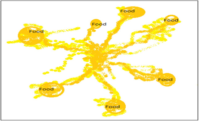
Searching structure of Physarum polycephalum (slime mold)

In the case of food scarcity, the slime mold even flows vibrantly, that helps to understand how slime mold search, moves, and connect food in the changing environment. When a secretion approaches the target, slime can judge the positive and negative feedback and find the ultimate route to grasp food in a better way. This suggests that slime mold can construct a concrete path subject to the level of food concentration. It prefers to select the region of high food concentration. Depending upon the food concentration and environmental risk, the mold weighs the speed and decides to leave the old location, and begins its new search during foraging [58]. Slime mold adopts empirical rules based on currently available insufficient data to decide to initialize new search and exit present location while foraging. Even if a food source is available in abundance, mold may divide its biomass to exploit other resources on the information of some rich high-quality food information. It may dynamically adjust their search patterns as per the quality of food stock [59].

Basic slime mold algorithm

Step 1 In this step, mathematics for the slime mold behavior is formed and following rule is assigned to find updated position of during search for food. The criteria for this depends upon r and p. This is the contraction mode of mold:

$$\overrightarrow{X(t+1)}=\left\{\begin{array}{cc}\overrightarrow{X_b(t)}+\overrightarrow{v_b}·\left(\overrightarrow{W}·\overrightarrow{X_A(t)}-\overrightarrow{X_B\left(t\right)}\right)& r<p\\ \overrightarrow{v_c}·\overrightarrow{X(t)}& r\ge p\end{array}\right),$$ 1

where $\overrightarrow{v_b}$ is a parameter with a range of $\left[-a,a\right],\overrightarrow{v_c}$ is the parameter which approaches linearly toward zero. ‘t’ is the current iteration, $\overrightarrow{X_b}$ is the location of each particle in region where odor is maximum, $\overrightarrow{X}$ is the mold’s location, ${\overrightarrow{X}}_A$ and ${\overrightarrow{X}}_B$ are the randomly selected variables from the swarm, $\overrightarrow{W}$ is the measure of weighs of masses.

The maximum limit of p is as follows:

$$p=tanh\left|S(i)-\text{DF}\right|,$$ 2

where $i\in 1,2,\dots ,n,$ $S(i)$ = fitness of $\overrightarrow{X}$, DF = overall fitness from all steps.

The equation of ${\overrightarrow{v}}_b$ as follows:

$$\overrightarrow{v_b}=\left[-a,a\right]$$ 3

$$a=arctanh\left(-\left(\frac{t}{max\_t}\right)+1\right).$$ 4

The equation of $\overrightarrow{W}$ is listed as follows:

$$\overrightarrow{W(\text{smell}\text{index}(i))}=\left\{\begin{array}{cc}1+r·log\left(\frac{\text{bF}-S(i)}{\text{bF}-\text{wF}}+1\right),& \text{condition}\\ 1-r·log\left(\frac{\text{bF}-S(i)}{\text{bF}-\text{wF}}+1\right),& \text{others}\end{array}\right),$$ 5

$$\text{Smell}\text{Index}=\text{sort}(S),$$ 6

where $S(i)$ rank first half of the population, r is the random value in the interval of $\left[0,1\right],$ $\text{bF}$ is the optimal fitness obtained in the current iterative process, $\text{wF}$ is the worst fitness value obtained in the iterative process, and Sort (s) function sorts fitness values.

Step 2 The equation for upgrading the positions of agents (i.e. to wrap food) is given as follows:

$$\overrightarrow{X^{\ast }}=\left\{\begin{array}{cc}\text{rand}·\left(\text{UB}-\text{LB}\right)+\text{LB},& \text{rand}<z\\ \overrightarrow{X_b(t)}+\overrightarrow{v_b}·(W·\overrightarrow{X_A(t)}-\overrightarrow{X_B(t)},& r<p\\ \overrightarrow{v_c}·\overrightarrow{X(t)},& r\ge p\end{array}\right),$$ 7

where LB and UB are the search limits, and rand and r denote the random value in [1].

Step 3 With the up gradation in the search process, the value of $\overrightarrow{v_b}$ vibrantly changes between $\left[-a,a\right]$ and $\overrightarrow{v_c}$ varies between $\left[-1,1\right]$ and at last shrinks to zero. This is known to be as ‘grabbling of food’.

Types of chaotic functions

The concept of probability distribution is captured by lot of meta-heuristics algorithms to gain randomness. Chaotic maps could be beneficial if randomness due to ergodicity, idleness and molding properties are replaced. These criteria’s are full filled by the following equation:

$$y_{k+1}=f(y_k).$$ 8

In Eq. (8), $y_{k+1}\text{and}f(y_k)$ are the (k + 1)th and Kth chaotic number, respectively. The action of chaotic function is dependent on initial value $y_0$. The particular type of chaotic function will generate a solution within the standardized equations as shown in Table 3.

Table 3.

Chaotic map functions

Sr. no.	Chaotic name	Mathematical description	Chaotic description
1	Chebyshev	$y_{i+1}=cos\left({cos}^{-1}\left(y_i\right)\right)$	$\left[-1,1\right]$
2	Iterative	$y_{i+1}=\text{Sin}\left(\raisebox{1ex}{$a\pi $}\!\left/ \!\raisebox{-1ex}{$y_i$}\right.\right),a=0.7$	$\left[-1,1\right]$
3	Sinusoidal	$y_{i+1}=a{x}_i\text{Sin}\left(\pi xi\right);a=2.3$	$\left[0,1\right]$
4	Sine	$y_{i+1}=\frac{a}{4}\text{Sin}\left(\pi yi\right),a=4$	$\left[0,1\right]$
5	Circle	$y_{i+1}=mod(y_i+b-\left(\raisebox{1ex}{$a$}\!\left/ \!\raisebox{-1ex}{$2\pi $}\right.\right)\text{Sin}\left(2\pi y_i\right),\left(1\right);a=0.5,b=0.2$	$\left[0,1\right]$
6	Piecewise	$\left\{\begin{array}{cc}\raisebox{1ex}{$y_i$}\!\left/ \!\raisebox{-1ex}{$p$}\right.& 0\le y_i⟨p\\ \raisebox{1ex}{$\left(y_i-p\right)$}\!\left/ \!\raisebox{-1ex}{$\left(0.5-p\right)$}\right.& p\le y_i⟨0.5\\ \raisebox{1ex}{$\left(1-p-y_i\right)$}\!\left/ \!\raisebox{-1ex}{$\left(0.5-p\right)$}\right.& 0.5\le y_i⟨1-p\\ \raisebox{1ex}{$\left(1-y_i\right)$}\!\left/ \!\raisebox{-1ex}{$p$}\right.& 1-p\le y_i⟨1,p=0.4\end{array}\right)$	$\left[0,1\right]$
7	Gauss/mouse	$\left\{\begin{array}{cc}1,& y_i=0\\ \frac{1}{mod\left(y_i,1\right)}& \text{otherwise}\end{array}\right)$	$\left[0,1\right]$
8	Singer	$y_{i+1}=\mu \left(7.86y_i-23.3y_i^2+28.75y_i^3-13.301875y_i^4\right),\mu =1.07$	$\left[0,1\right]$
9	Logistic	$y_{i+1}=a{y}_i\left(1-y_i\right),a=4$	$\left[0,1\right]$
10	Tent	$y_{i+1}=\left\{\begin{array}{cc}\left(y_i/0.7\right),& y_i<0.7\\ \left(10/3\right)\left(1-y\right),& y_i\ge 0.7\end{array}\right)$	$\left[0,1\right]$

Algorithm of proposed work

The basic SMA is combined with the sinusoidal chaotic approach to further enhance the performance. The pseudo-code for method proposed is as shown in Fig. 2.

Fig. 2.

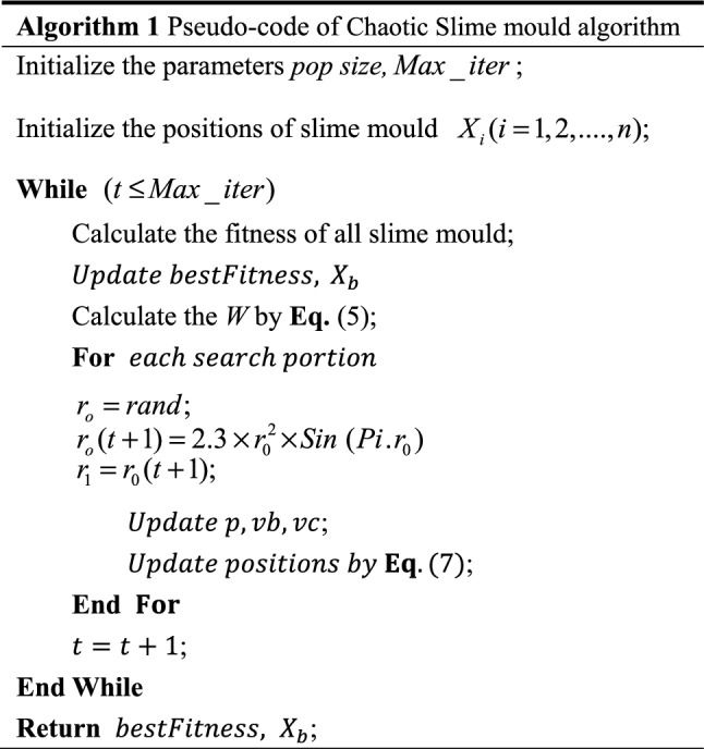
Pseudo-code of chaotic slime mold algorithm

There are several complex optimization problems wherein mathematical reformulations restrict to perform algorithms efficiently. The proposed Chaotic SMA variant is advantageous over standard algorithms along with standard SMA. The convergence rate of stochastic methods was noticed not much efficient due to premature convergence. Whenever some additional functionality is incorporated with the original system, the performance starts getting degraded. After a thorough review of various SMA and chaotic variants, it is observed that the sinusoidal function to be the most appropriate to improve exploitation. The proposed algorithm utilizes a sinusoidal chaotic function to intensify the search capacity of classical SMA and optimize the objective fitness of various problems. The chaotic approach enables SMA to regulate the initial parameters of the search and thus rectifies the local entrapment of molds. It is seen that some algorithms lack global search capability. For the efficient performance of any algorithm, there should a proper balance between its local and global search capabilities. In the proposed research, to incorporate these local and global search requirements, no composite operations are involved. Second, the efficacy of any algorithm is judged by the simulation time required to simulate a particular objective function. The experimental section of the paper reveals that the suggested method has improved solution efficacy to a greater extend. Lastly, during the cumulative run process, as the simulation successive progresses, premature convergence “local area stagnation” is the most common problem of many algorithms. This local area stagnation problem is omitted in the proposed method by utilizing the properties of ergodicity. The basic feature of Chaotic SMA is to enhance the optimization process by improving local search capabilities. Twenty-three benchmark problems including uni-modal, multi-modal and fixed dimensions are tested using the suggested chaotic slime algorithm.

Test benchmark functions

The developed Chaotic SMA algorithm has been simulated on Intel Core TM, i5-3320 M CPU@2.60 GHz system. These standard benchmark function are characterized by their objective fitness in parameter space within a particular dimension (Dim), range, and frequency ($f_{min}$). In the entire work, F1–F7 represent as uni-modal test functions (U-Modal), F8–F13 are multi-modal test functions (M-Modal) and F14–F23 are fixed dimension (FD) functions. The effectiveness of the proposed Chaotic SMA optimization technique is examined by referring benchmark functions are taken [91, 92]. The characteristics of benchmark functions differ from each other. Some functions show better performance in exploring local search while a few functions are found to excellent in determining global optima. Table 4 illustrates equations of F1–F7 with their name, dimension, range, and frequency. On similar grounds, Tables 5 and 6 explore the details of multi-modal and fixed dimensions functions.

Table 4.

Standard uni-modal benchmark

Uni-modal test function	Name	Dim	Limit	$f_{min}$
$f_1(y)={\sum }_{i=1}^n{y}_i^2$	Sphere function	30	[− 100, 100]	0
$f_2(y)={\sum }_{i=1}^n\left|y_i\right|+{\prod }_{i=1}^n\left|y_i\right|$	Schwefel absolute function	30	[−10, 10]	0
$f_3(y)={\sum }_{i=1}^n{\left({\sum }_{j=1}^i{y}_j\right)}^2$	Schwefel double sum function	30	[− 100, 100]	0
$f_4(y)={max}_i\left\{\left|y_i\right|,1\le i\le n\right\}$	Schwefel max. function	30	[− 100, 100]	0
$f_5(y)={\sum }_{i=1}^{n-1}\left[100{(y_{i+1}-y_i^2)}^2+{(y_i-1)}^2\right]$	Rosenbrock function	30	[−30, 30]	0
$f_6(y)={\sum }_{i=1}^n{\left(\left[y_i+0.5\right]\right)}^2$	The step function	30	[−100, 100]	0
$f_7(y)={\sum }_{i=1}^{n}i{y}_i^4+\text{random}\left[0,1\right]$	Quartic random function	30	[−1.28, 1.28]	0

Table 5.

Multimodal test function (M-modal)

Multimodal test function	Name	Dim	Limit	$f_{min}$
$f_8(y)={\sum }_{i=1}^n-y_{i}sin(\sqrt{\left|y_i\right|})$	Schwefel sine function	30	[-500, 500]	− 418.98295
$f_9(y)={\sum }_{i=1}^n[y_i^2-10cos(2\pi y_i)+10]$	Rastrigin function	30	[− 5.12, 5.12]	0
$f_{10}(y)=-20exp\left(-0.2\sqrt{\frac{1}{n}{\sum }_{i=1}^n{y}_i^2}\right)-exp\left(\frac{1}{n}{\sum }_{i=1}^{n}cos(2\pi y_i)+20+c\right)$	The Ackley function	30	[− 32, 32]	0
$f_{11}(y)=1+{\sum }_{i=1}^n\frac{y_i^2}{4000}-{\prod }_{i=1}^{n}cos\frac{(y_i)}{\sqrt{i}}$	Griewank function	30	[− 600, 600]	0
$f_{12}(y)=\frac{\pi }{n}\left\{10sin(\pi y_1)+{\sum }_{i=1}^{n-1}{(y_i-1)}^2[1+10{sin}^2(\pi z_{i+1})]+{(z_n-1)}^2\right\}+{\sum }_{i=1}^{n}u(y_i,10,100,4)$$z_1=1+\frac{y_i+1}{4}$ $u(y_{i,}a,k,m)=\left\{\begin{array}{c}k{(y_i-a)}^n{y}_i>a\\ 0-a<y_i<a\\ k{(-y_i-a)}^n{y}_i<-a\end{array}\right)$	Penalized Penalty#1 function	30	[− 50, 50]	0
$F_{13}(x)=0.1\left\{{sin}^2\left(3\pi x_1\right)+{\sum }_{i=1}^n\begin{array}{c}{\left(x_i-1\right)}^2\left[1+{sin}^2\left(3\pi x_i+1\right)\right]+\\ {(x_n-1)}^2\left[1+{sin}^2(2\pi x_n)\right]\\ \end{array}\right\}+{\sum }_{i=1}^{n}u(x_i,5,100,4)$	Levi N. 13 function	30	[− 50, 50]	0

Table 6.

Fixed dimension test function

FD test function	Name	Dim	Limit	fmin
$f_{14}(y)={\left[\frac{1}{500}+{\sum }_{j=1}^{2}5\frac{1}{j+{\sum }_{i=1}^n{(y_i-a_{\mathit{ij}})}^6}\right]}^{-1}$	Shekel foxhole Function	2	[− 65.536, 65.536]	1
$f_{15}(y)={\sum }_{i=1}^{11}{\left[a_i-\frac{y_1\left(b_i^2+b_i{y}_2\right)}{b_i^2+b_i{y}_3+y_4}\right]}^2$	Brad function	4	[− 5, 5]	0.00030
$f_{16}(y)=4y_1^2-2.1y_1^4+\frac{1}{3}{y}_1^6+y_1{y}_2-4y_2^2+4y_2^4$	Camel function—six hump	2	[− 5, 5]	− 1.0316
$f_{17}(y)={\left(y_2-\frac{5.1}{4{\pi }^2}{y}_1^2+\frac{5}{\pi }{y}_1-6\right)}^2+10\left(1-\frac{1}{8\pi }\right)cos{y}_1+10$	Branin RCOS function	2	[− 5, 5]	0.398
$f_{18}(y)=\left[\begin{array}{c}1+{(y_1+y_2+1)}^2\\ \left(19-14y_1+3y_1^2-14y_2+6y_1{y}_2+3y_2^2\right)\\ \end{array}\right]\times \left[\begin{array}{c}30+{\left(2y_1-3y_2\right)}^2\times \\ \left(\begin{array}{c}18-32y_1+12y_1^2+48y_2\\ -36y_1{y}_2+27y_2^2\\ \end{array}\right)\\ \end{array}\right]$	Goldstein-price function	2	[− 2, 2]	3
$f_{19}(y)=-{\sum }_{i=1}^4{c}_{i}exp\left(-{\sum }_{j=1}^3{a}_{\mathit{ij}}{(y_j-q_{\mathit{ij}})}^2\right)$	Hartman 3 function	3	[1, 3]	− 3.32
$f_{20}(y)=-{\sum }_{i=1}^4{c}_{i}exp\left(-{\sum }_{j=1}^6{a}_{\mathit{ij}}{(y_j-q_{\mathit{ij}})}^2\right)$	Hartman 6 function	6	[0, 1]	− 3.32
$f_{21}(y)=-{\sum }_{i=1}^5{\left[\begin{array}{c}(y-a_i){}_{}\\ {(y-a_i)}^T+d_i\\ \end{array}\right]}^{-1}$	Hybrid composition function #1	4	[0, 10]	− 10.1532
$f_{22}(y)=-{\sum }_{i=1}^7{\left[\begin{array}{c}(y-a_i){}_{}\\ {(y-a_i)}^T+d_i\\ \end{array}\right]}^{-1}$	Hybrid composition function #2	4	[0, 10]	− 10.4028
$f_{23}(y)=-{\sum }_{i=1}^{10}{\left[\begin{array}{c}(y-a_i)\\ {(y-a_i)}^{\text{T}}+d_i\\ \end{array}\right]}^{-1}$	Hybrid composition function #3	4	[0, 10]	− 10.5363

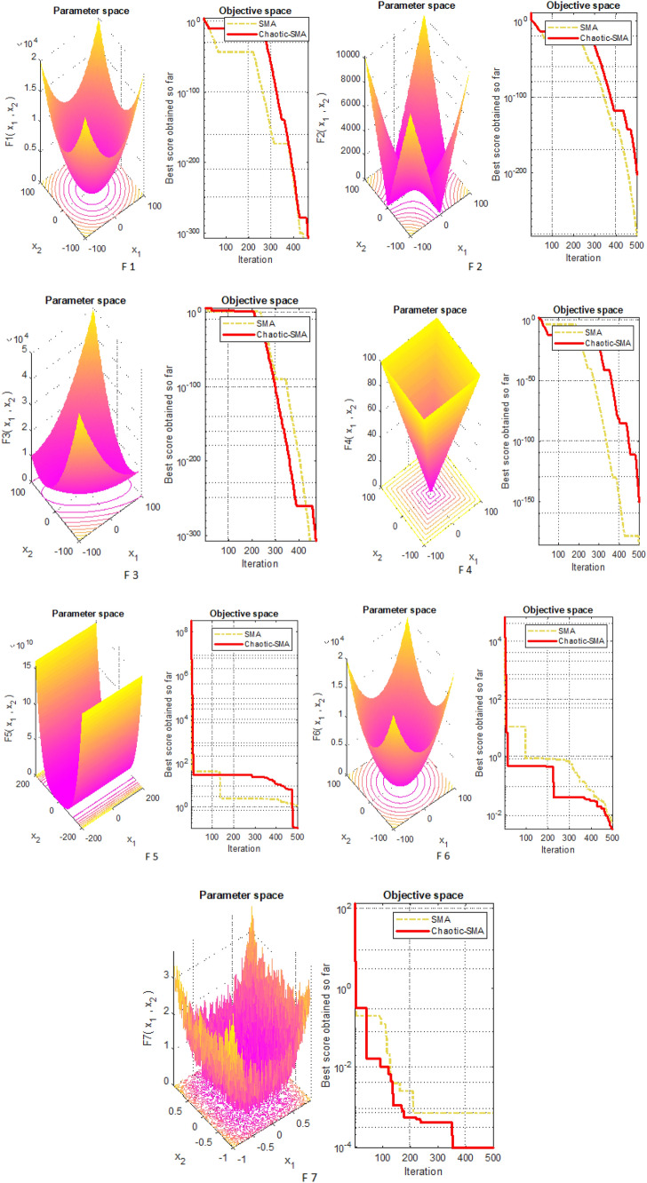
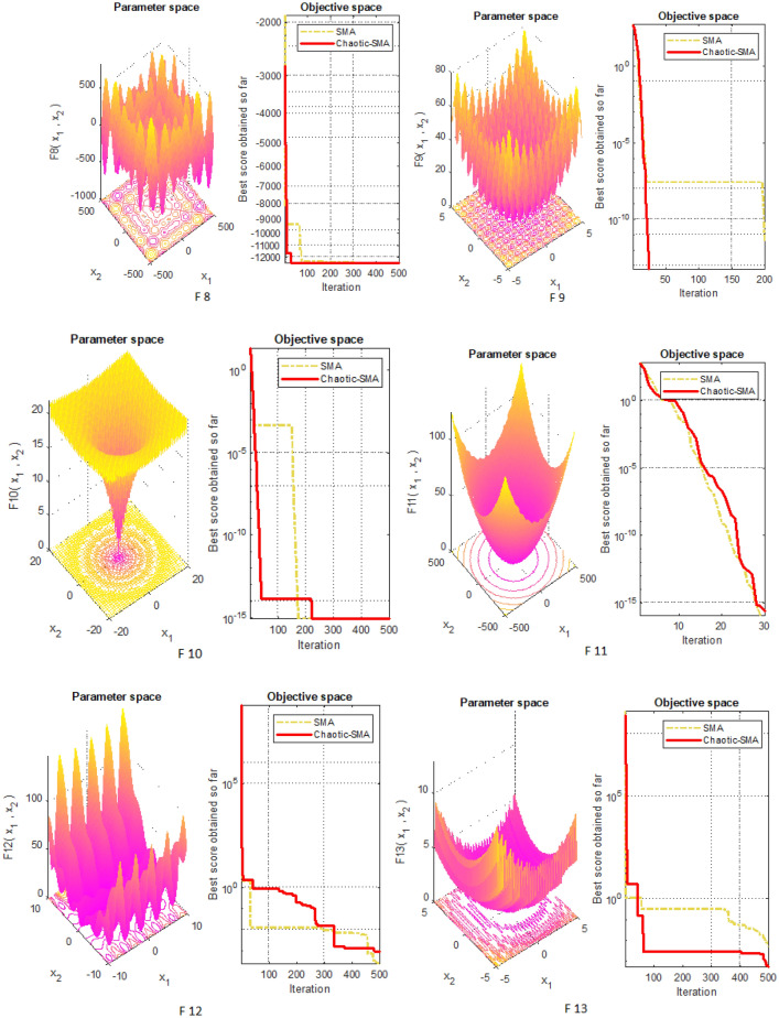
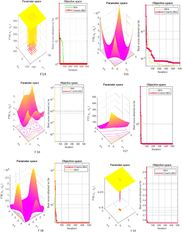
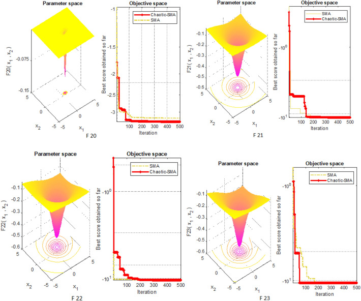
In the whole research study, 30 search agents are taken into considerations and the proposed algorithm is simulated for maximum iterations of 500. Figures 3, 4, and 5 illustrate the 3D view along with their objective space representing convergence for F1–F7, F8–F13 and F14–F23, respectively. It is clear from the various comparative results that the newly developed chaotic strategy appreciably increases convergence rate and thus improves its ability to easily escape from local minima entrapment.

Fig. 3.

Three-dimensional view of F1–F7 along with convergence curve for SMA and CSMA

Fig. 4.

Three-dimensional view of F8–F13 along with convergence curve for SMA and CSMA

Fig. 5.

Three-dimensional view of F14–F23 along with convergence curve for SMA and CSMA

Results of proposed algorithm

In this section, test results for benchmark functions are discussed with their average, best, worst, median, standard deviation, and p value have been taken into account. The stochastic complexity of the proposed algorithm is justified and analyzed by running the algorithm for 30 trial checks and 500 iterations. To analyze the feasibility of the solution, Wilcoxon sum test has been taken into account. The parameter setting for the proposed CSMA method is illustrated in Table 7. On similar grounds, results are compared with other universally validated systems.

Table 7.

Parameter setting for the proposed method

Parameter setting	CSMA
Number of search agents	30
Number of iterations for U-Modal, M-modal, and F-Modal	500
Number of iterations for engineering optimization design problems	500
Number of trial runs test functions	30
Number of trial engineering design problems	30

Testing of uni-modal functions (U-modal)

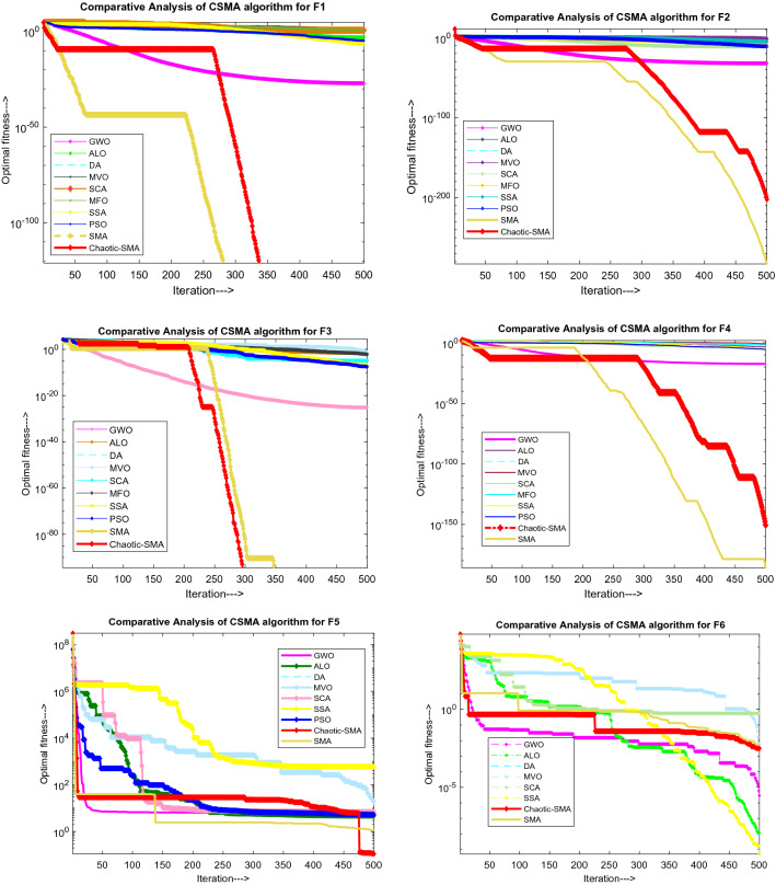
The search process for the best position depends upon the capability of the search agents to reach closer to origin. During the search process by various agents, there may be the possibility of getting entrap far or nearby and accordingly defined in terms of exploration and exploitation. Exploration comes under the global search process and exploitation falls under the local search category. The statistical outcomes of U-Modal (F1–F7) have a few pick points with increased convergence validates the effectiveness of the proposed algorithm. Figure 6 illustrates a comparison between Chaotic SMA and different methods. It can be seen from the convergence curves that the suggested algorithm converges to optima much earlier.

Fig. 6.

Convergence curve for U-Modal test function showing comparison of CSMA with other algorithms

To check the appropriateness of the proposed algorithm, each test function is simulated with SMA and CSMA. Table 8 illustrates statistical outcomes of the uni-modal benchmark function in terms of average, standard deviation, the best value, worst value, median value, and p value. In the search space, there are some regions of global optima whereas some regions are stagnated to local optima. The global search process determines the exploration phase whereas in the local search process, exploitation phase is evaluated. The performance of any algorithm is judged by its ability to attain the maxima or minima with less computation time. Table 9 shows the computational time in terms of best, mean, and worst time. Table 10 shows the comparison of the CSMA method with other techniques such as PSO [93], GWO [15], GSA [94], BA [95], FA [96], GA [97], BDA [98], BPSO [99], MFO [16], MVO [6], BGSA [100], SMS [101], FPA [102], DE [103], ALO [104], and WOA [105] in terms of average (AVG) and standard deviation (SD).

Table 8.

Test results for U-modal function using CSMA

Functions	Average value	STD	Best value	Worst value	Median value	p value
F1	1.2E−280	0	0	3.5E−279	0	0.5
F2	3.4E−156	1.7E−155	3E−258	9.4E−155	1.3E−188	1.7344E−06
F3	0	0	0	0	0	1
F4	5.1E−134	2.8E−133	1.5E−269	1.5E−132	2.7E−190	1.7344E−06
F5	5.035453	9.27916	0.044388	28.19006	1.219173	1.7344E−06
F6	0.004431	0.003059	2.06E−05	0.016714	0.004434	1.7344E−06
F7	0.0003	0.000211	2.17E−05	0.000935	0.000274	1.7344E−06

Table 9.

Simulation time for uni-modal benchmark problems using CSMA

Functions	Best time (s)	Mean time (s)	Worst time (s)
F1	2.71875	2.915625	3.453125
F2	2.78125	2.890625	3.375
F3	2.984375	3.295313	4.078125
F4	2.84375	3.039583	3.875
F5	2.84375	2.991667	3.578125
F6	2.8125	2.955208	3.453125
F7	2.9375	3.077604	3.59375

Table 10.

Comparative results of U-Modal test function

Algorithm	Parameters	Uni-modal test function
		F1	F2	F3	F4	F5	F6	F7
PSO [93]	AVG	1.3E−04	0.04214	7.01256E+01	1.08648	96.7183	0.00010	0.12285
	SD	0.0002.0E−04	0.04542	2.1192E+01	3.1703E+01	6.01155E+01	8.28E−05	0.04495
GWO [15]	AVG	6.590E−29	7.180E−18	3.20E−07	5.610E−08	26.8125	0.81657	0.00221
	SD	6.3400E−07	0.02901	7.9.1495E+01	1.31508	69.9049	0.00012	0.10028
GSA [4]	AVG	2.530E−17	0.05565	896.534	7.35487	6.7543E+01	2.500E−17	0.08944
	SD	9.670E−18	0.19407	318.955	1.741452	6.2225E+01	1.740E−17	0.04339
DE [1]	AVG	8.200E−15	1.50E−09	6.80E−11	0.00	0.00	0.00	0.00463
	SD	5.900E−15	9.900E−11	7.40E−11	0.00	0.00	0.00	0.0012
FEP [91]	AVG	0.0005	0.0081	0.016	0.3	5.06	0.00	0.1415
	SD	0.0001	0.0007	0.014	0.5	5.87	0.00	0.3522
ALO [104]	AVG	2.59E−10	1.84E−06	6.07E−10	1.36E−08	0.3467724	2.56E−10	0.00429249
	SD	1.65E−10	6.58E−07	6.34E−10	1.81E−09	0.10958	1.09E−10	0.00508
BA [14]	AVG	0.77362	0.33458	0.11530	0.19218	0.33407	0.77884	0.13748
	SD	0.52813	3.81602	0.76603	0.890266	0.30003	0.67392	0.11267
CS [106]	AVG	0.0065	0.212	0.247	1.120E−06	0.00719	5.95E−06	0.00132
	SD	0.00020	0.0398	0.0214	8.250E−07	0.00722	1.08E−07	0.00072
GOA [42]	AVG	0.000	0.002	0.001	0.000	0.000	0.000	0.000
	SD	0.000	0.001	0.0203	0.000	0.000	0.000	0.000
MFO [16]	AVG	0.00011	0.00063	696.730	70.6864	139.1487	0.000113	0.091155
	SD	0.00015	0.00087	188.527	5.27505	120.2607	9.87E−05	0.04642
MVO [6]	AVG	2.08583	15.9247	453.200	3.12301	1272.13	2.29495	0.05199
	SD	0.64865	44.7459	177.0973	1.58291	1479.47	0.63081	0.02961
DA [98]	AVG	2.850E−19	1.490E−06	1.290E−07	9.88E−04	7.6	4.170E−17	1.03E−02
	SD	7.160E−19	3.760E−06	2.100E−07	2.78E−03	6.79	1.320E−16	4.69E−03
BDA [98]	AVG	2.82E−01	5.89E−02	1.4E+01	2.48E−01	2.36E−01	9.53E−02	1.22E−02
	SD	4.18E−02	6.93E−02	2.27E+01	0.331	34.7	0.13	0.0146
BPSO [107]	AVG	5.59	0.196	15.5	1.9	86.4	6.98	0.0117
	SD	1.98	0.0528	13.7	0.484	65.8	3.85	0.00693
BGSA [100]	AVG	83	1.19	456	7.37	3100	107	0.0355
	SD	49.8	0.228	272	2.21	2930	77.5	0.0565
SCA [108]	AVG	0.000	0.000	0.0371	0.0965	0.0005	0.0002	0.000
	SD	0.000	0.0001	0.1372	0.5823	0.0017	0.0001	0.0014
SSA [109]	AVG	0.000	0.2272	0.000	0.000	0.000	0.000	0.0028
	SD	0.000	1.000	0.000	0.6556	0.000	0.000	0.007
WOA [105]	AVG	1.410E−31	1.060E−22	5.390E−08	7.258E−02	27.8655	3.11626	0.00142
	SD	4.910E−31	2.390E−22	2.930E−07	3.9747E−01	7.6362E−01	0.53242	0.00114
CSMA	AVG	1.2E−280	3.4E−156	0	5.1E−134	5.035453	0.004431	0.0003
	SD	0	1.7E−155	0	2.8E−133	9.27916	0.003059	0.00021

Bold values indicate the results of the Chaotic variant of the Slime Mould Algorithm

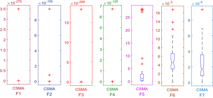
The characteristics of benchmark functions vary from each other. These test functions have different exploration and exploitation search capacities. Griewank, levy, Ackley, Rastrigin, Schwefel functions, sphere function, explore many local minima points while sum square function, Zakharov are applicable to explore global minima points. In this regard, test assessment of seven uni-modal benchmark functions (F1–F7) are analyzed. The test results for each function in terms of average and standard deviations over 30 independent trial runs and 500 iterations are recorded. The scalability assessment is carried out to investigate the impact of chaos on the solutions of SMA. The statistical results shown in Table 10 reveals an appreciable gap between CSMA and other methodologies. As it can be seen in Table 10, that by introducing a chaotic function, the exploration and exploitation phase of SMA has been improved. The results of CSMA when compared with PSO, GWO, DE, FA, GA, BBO, MFO, SCA, and SSA show remarkable performance in dealing with F3, F4, and F7 test functions. As per the convergence curves in Fig. 6, it is observed that the optimality of results is increased with higher efficiency. On the other hand, the former method are found to be subjected to premature convergence. Further, to verify the effectiveness of the proposed method, independent trial runs for each benchmark function are illustrated in Fig. 7. Comparative analysis revealed that the sinusoidal chaotic function facilitates to explore the local search phase more intensively.

Fig. 7.

Trial runs of Uni-modal benchmark function

Testing of multi-modal test functions (M-modal)

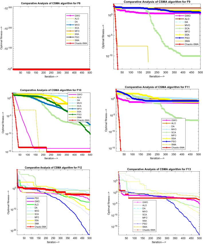
Figure 8 illustrates comparison between Chaotic SMA and other methods for multi-modal benchmark (F8–F13).The multi-modal function is tested for 30 introductory attempts and 500 iterations and results are shown in Table 11. Simulation time for M-Modal utilizing CSMA appears in Table 12. Table 13 shows compared results with other meta-heuristics search algorithms such as PSO [93], GWO [15], GSA [94], BA [95], FA [96], GA [97], BDA [98], BPSO [99], MFO [16], MVO [6], BGSA [100], SMS [101], FPA [102], DE [103], ALO [104], and WOA [105] in terms of average value and std. deviation. It can be seen Fig. 8 that test outcomes of M-Modal (F8–F13) have some pick points with increased convergence using CSMA, justifies the effectiveness of algorithm in solving multi-modal test functions.

Fig. 8.

Convergence curve for M-Modal test function showing comparison of CSMA with other algorithms

Table 11.

Testing of multi-modal using CSMA

Functions	Average value	STD	Best value	Worst value	Median value	p value
F8	− 12,569.1	0.319584	− 12,569.5	− 12,568.1	− 12,569.2	1.7344E−06
F9	0	0	0	0	0	1
F10	8.88E−16	0	8.88E−16	8.88E−16	8.88E−16	4.32046E−08
F11	0	0	0	0	0	1
F12	0.003937	0.006237	5.64E−07	0.032017	0.002066	1.7344E−06
F13	0.00664	0.00989	7.428E−05	0.05034892	0.00270	1.7344E−06

Table 12.

Simulation time for M-modal using CSMA

Functions	Best time	Mean time	Worst time
F8	2.796875	2.929167	3.421875
F9	2.765625	2.911458	3.546875
F10	2.828125	2.948438	3.40625
F11	2.84375	2.996875	3.6875
F12	3.09375	3.206771	3.765625
F13	3.09375	3.198958	3.765625

Table 13.

Comparison of multi-modal test function

Algorithms	Parameters	M-modal
		F8	F9	F10	F11	F12	F13
GWO [15]	AVG	− 6.1200E+02	3.1100E−02	1.0600E−14	4.4900E−04	5.3400E−03	6.5400E−02
	SD	− 4.0900E+02	4.740E+01	7.7800E−03	6.6600E−04	2.0700E−03	4.470E−03
PSO [10]	AVG	− 4.8400E+04	4.670E+01	2.760E−01	9.2200E−04	6.9200E−04	6.6800E−04
	SD	1.1500E+04	1.160E+01	5.090E−01	7.7200E−04	2.6300E−03	8.9100E−04
GSA [4]	AVG	− 2.820E+03	2.600E+01	6.210E−02	2.770E+01	1.800E+00	8.900E+00
	SD	4.930E+02	7.470E+00	2.360E−01	5.040E+00	9.510E−01	7.130E+00
DE [1]	AVG	− 1.110E+04	6.920E+01	9.700E−08	0.000E+00	7.900E−15	5.100E−14
	SD	5.750E+02	3.880E+01	4.200E−08	0.000E+00	8.000E−15	4.800E−14
FEP [91]	AVG	− 1.2600E+03	4.6000E−01	1.8000E−03	1.6000E−03	9.2000E−05	1.6000E−05
	SD	5.260E+00	1.200E−03	2.100E−02	2.200E−03	3.600E−05	7.300E−06
ALO [104]	AVG	− 1.61E+03	7.71E−06	3.73E−15	1.86E−02	9.75E−12	2.00E−11
	SD	3.14E+02	8.45E−06	1.50E−15	9.55E−03	9.33E−12	1.13E−11
SMS [101]	AVG	− 4.21E+00	1.33E+00	8.88E−06	7.06E−01	1.23E−01	1.35E−02
	SD	9.36E−16	3.26E−01	8.56E−09	9.08E−01	4.09E−02	2.88E−04
BA [14]	AVG	− 1.070E+03	1.230E+00	1.290E−01	1.450E+00	3.960E−01	3.870E−01
	SD	8.580E+02	6.860E−01	4.330E−02	5.700E−01	9.930E−01	1.220E−01
CS [96]	AVG	− 2.090E+03	1.270E−01	8.160E−09	1.230E−01	5.600E−09	4.880E−06
	SD	7.620E−03	2.660E−03	1.630E−08	4.970E−02	1.580E−10	6.090E−07
GA [110]	AVG	− 2.090E+03	6.590E−01	9.560E−01	4.880E−01	1.110E−01	1.290E−01
	SD	2.470E+00	8.160E−01	8.080E−01	2.180E−01	2.150E−03	6.890E−02
GOA [42]	AVG	1.000E+00	0.000E+00	9.750E−02	0.000E+00	0.000E+00	0.000E+00
	SD	2.000E−04	7.000E−04	1.000E+00	0.000E+00	7.000E−04	0.000E+00
MFO [16]	AVG	− 8.500E+03	8.460E+01	1.260E+00	1.910E−02	8.940E−01	1.160E−01
	SD	7.260E+02	1.620E+01	7.300E−01	2.170E−02	8.810E−01	1.930E−01
MVO [6]	AVG	− 1.170E+04	1.180E+02	4.070E+00	9.400E−01	2.460E+00	2.200E−01
	SD	9.370E+02	3.930E+01	5.500E+00	6.000E−02	7.900E−01	9.000E−02
DA [98]	AVG	− 2.860E+03	1.600E+01	2.310E−01	1.930E−01	3.110E−02	2.200E−03
	SD	3.840E+02	9.480E+00	4.870E−01	7.350E−02	9.830E−02	4.630E−03
BDA [98]	AVG	− 9.240E+02	1.810E+00	3.880E−01	1.930E−01	1.490E−01	3.520E−02
	SD	6.570E+01	1.050E+00	5.710E−01	1.140E−01	4.520E−01	5.650E−02
BPSO [107]	AVG	− 9.890E+02	4.830E+00	2.150E+00	4.770E−01	4.070E−01	3.070E−01
	SD	1.670E+01	1.550E+00	5.410E−01	1.290E−01	2.310E−01	2.420E−01
BGSA [100]	AVG	− 8.610E+02	1.030E+01	2.790E+00	7.890E−01	9.530E+00	2.220E+03
	SD	8.060E+01	3.730E+00	1.190E+00	2.510E−01	6.510E+00	5.660E+03
SCA [108]	AVG	1.000E+00	0.000E+00	3.800E−01	0.000E+00	0.000E+00	0.000E+00
	SD	3.600E−03	7.300E−01	1.000E+00	5.100E−03	0.000E+00	0.000E+00
SSA [109]	AVG	5.570E−02	0.000E+00	1.950E−01	0.000E+00	1.420E−01	8.320E−02
	SD	8.090E−01	0.000E+00	1.530E−01	6.510E−02	5.570E−01	7.060E−01
WOA [105]	AVG	− 5.080E+03	0.000E+00	7.400E+00	2.890E−04	3.400E−01	1.890E+00
	SD	6.960E+02	0.000E+00	9.900E+00	1.590E−03	2.150E−01	2.660E−01
CSMA	AVG	− 12,569.1	0	8.88E−16	0	0.003937	0.00664
	SD	0.319584	0	0	0	0.006237	0.00989

Bold values indicate the results of the Chaotic variant of the Slime Mould Algorithm

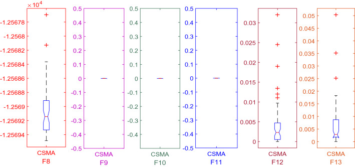
From the statistical data analysis illustrated in Table 13, it is observed that the optimality of multi-modal test functions is marginally improved by implementing the sinusoidal chaotic function. According to the best and standard deviation results, CSMA shows better performance for almost all seven test functions. As can be seen from convergence curves shown in Fig. 8, CSMA gives optimal convergences except for a few of the test functions. It can be understood from the convergence comparison that CSMA converges faster and seizes the run as soon as it reaches the stop criterion. As per comparative curves shown in Fig. 8, it is observed that the suggested algorithm shows superior performance in dealing with F9, F10 and F11 and comparative operation in the case of F8, F12 and F13. Trial run accuracy matrices shown in Fig. 9 reveal that proposed CSMA significantly searches the local and global space more intensively.

Fig. 9.

Trial runs of M-Modal functions

Testing of fixed dimension function (F-modal)

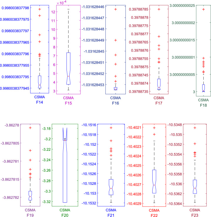
Fixed dimension test functions (F14–F23) are tested for 30 trial runs and 500 iterations as shown in Fig. 11. Simulation results for FD test function using CSMA are shown in Table 14. Table 15 illustrates simulation results of F-Modal. It can be seen that results for F-Modal have many pick points with better convergence. Simulation time for F-Modal benchmark problems using CSMA is shown in Table 15. Table 16 illustrates CSMA results compared with others variants such as GWO [15], PSO [10], GSA [4], DE [1], and FEP [91] in terms of average (AVG) and standard deviation (SD).

Fig. 11.

Trial run of FD benchmark functions

Table 14.

Simulation results for fixed dimension test function using CSMA

Functions	AVG	SD	Best value	Worst value	Median value	p value
F14	0.998004	9.26E−13	0.998004	0.998004	0.998004	1.7344E−06
F15	0.00055	0.000244	0.00031	0.001223	0.000469	1.7344E−06
F16	− 1.03163	1.51E−09	− 1.03163	− 1.03163	− 1.03163	1.7344E−06
F17	0.397887	6.82E−08	0.397887	0.397888	0.397887	1.7344E−06
F18	3	8.43E−12	3	3	3	1.7344E−06
F19	− 3.86278	4.21E−07	− 3.86278	− 3.86278	− 3.86278	1.7344E−06
F20	− 3.25824	0.060654	− 3.32199	− 3.20008	− 3.20309	1.7344E−06
F21	− 10.1528	0.000274	− 10.1532	− 10.1519	− 10.1529	1.7344E−06
F22	− 10.4026	0.000208	− 10.4029	− 10.4021	− 10.4027	1.7344E−06
F23	− 10.536	0.000299	− 10.5364	− 10.5354	− 10.5361	1.7344E−06

Table 15.

Simulation time for fixed dimension using CSMA

Functions	Best time	Mean time	Worst time
F14	1.140625	1.215104	1.921875
F15	0.671875	0.788021	1.34375
F16	0.53125	0.623438	1.171875
F17	0.5	0.582813	1.21875
F18	0.5	0.595313	1.125
F19	0.59375	0.680729	1.265625
F20	0.859375	0.971354	1.46875
F21	0.8125	0.941146	1.4375
F22	0.859375	0.972917	1.40625
F23	0.9375	1.065104	1.59375

Table 16.

Comparison of FD test function with other methods

Algorithms	Parameter	FD test function
		F14	F15	F16	F17	F18	F19	F20	F21	F22	F23
GWO [15]	AVG	4.04	0.00	− 1.03	0.40	3.00	− 3.86	− 3.29	− 10.15	− 10.40	− 10.53
	SD	4.25	0.00	− 1.03	0.40	3.00	− 3.86	− 3.25	− 9.14	− 8.58	− 8.56
PSO [111]	AVG	3.63	0.00	− 1.03	0.40	3.00	− 3.86	− 3.27	− 6.87	− 8.46	− 9.95
	SD	2.56	0.00	0.00	0.00	0.00	0.00	0.06	3.02	3.09	1.78
GSA [4]	AVG	5.86	0.00	− 1.03	0.40	3.00	− 3.86	− 3.32	− 5.96	− 9.68	− 10.54
	SD	3.83	0.00	0.00	0.00	0.00	0.00	0.02	3.74	2.01	0.00
DE [1]	AVG	1.00	0.00	− 1.03	0.40	3.00	N/A	N/A	− 10.15	− 10.40	− 10.54
	SD	0.00	0.00	0.00	0.00	0.00	N/A	N/A	0.00	0.00	0.00
FEP [90]	AVG	1.22	0.00	− 1.03	0.40	3.02	− 3.86	− 3.27	− 5.52	− 5.53	− 6.57
	SD	0.56	0.00	0.00	0.00	0.11	0.00	0.06	1.59	2.12	3.14
CSMA (proposed method)	AVG	0.998004	0.00055	− 1.03163	0.397887	3	− 3.86278	− 3.25824	− 10.1528	− 10.4026	− 10.536
	SD	9.26E−13	0.000244	1.51E−09	6.82E−08	8.43E−12	4.21E−07	0.060654	0.000274	0.000208	0.000299

Bold values indicate the results of the Chaotic variant of the Slime Mould Algorithm

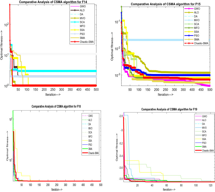
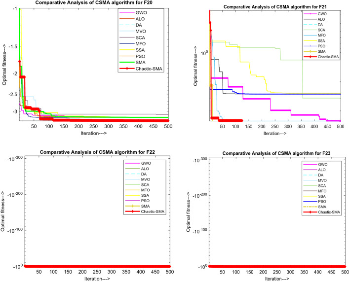
The statistical data analysis illustrated in Table 16 shows that solution accuracy of fixed dimension test functions is appreciably improved by implementing the sinusoidal chaotic function. Rendering to the best and standard deviation results, CSMA shows enhanced performance for nearly all ten test functions. As can be seen from convergence curves shown in Fig. 10, CSMA gives optimal convergences except for a few of the test functions. It can be implicit from the convergence evaluation that CSMA converges faster and seizes the run as soon as it reaches the halt criterion. As per comparative curves shown in Fig. 8, it is observed that the suggested algorithm shows superior performance in dealing with F14, F18, F19 and F20 and comparative operation in the case of F15, F21, F22 and F23. Trial runs shown in Fig. 11 reveal that proposed CSMA significantly searches the local and global space for finding the optimal solution.

Fig. 10.

Convergence curve for FD test function showing comparison of CSMA with other algorithms

Multi-disciplinary engineering design problems

In this section, ten real-world design problems are tested which includes “3-bar truss problem, pressure –vessel design, compression design, welded beam, cantilever beam design, gear train design problem, speed reducer problem, Belleville spring problem, rolling element problem and multidisc clutch brake problem” [112]. Each design problem is simulated with CSMA algorithm. The abbreviations for various multidisciplinary engineering functions (EFs) has been shown in Table 17. The comparison of the engineering design problem with their average, standard deviation, best, worst and p value has been elucidated in Table 18 and simulation time for best, mean and average values are shown in Table 19.

Table 17.

Abbreviations for 10 types of design problems

Engineering function (EF)	Type of problem
EF1	3-bar truss problem
EF2	Pressure vessel
EF3	Compression design
EF4	Welded beam
EF5	Cantilever beam design
EF6	Gear train
EF7	Speed reducer problem
EF8	Belleville spring
EF9	Rolling element bearing
EF10	Multiple disk clutch brake (discrete variables)

Table 18.

Engineering design problems by CSMA

Engineering function (EF)	Mean	STD value	Best value	Worst value	Median value	p value
EF1	270.7824	1.791805	265.4599	273.3948	271.2534	1.7344E−06
EF2	2994.48	0.005837	2994.474	2994.495	2994.479	1.7344E−06
EF3	6427.41	531.9222	5885.341	7318.996	6195.263	1.7344E−06
EF4	0.014245	0.001415	0.012715	0.017524	0.013955	1.7344E−06
EF5	1.740409	0.052373	1.724899	2.00749	1.726646	1.7344E−06
EF6	− 85,534.4	10.61208	− 85,539.2	− 85,498.2	− 85,538.7	1.7344E−06
EF7	0.392818	0.005457	0.389654	0.404654	0.389664	1.7344E−06
EF8	3.34E−11	6.46E−11	4.82E−14	2.91E−10	7.56E−12	1.7344E−06
EF9	5.24E+22	5.87E+22	1.57E+21	1.79E+23	1.21E+22	1.7344E−06
EF10	1.303713	0.000368	1.303281	1.30519	1.303612	1.7344E−06

Table 19.

Computation time for engineering function (EF) using CSMA

Functions	Best time	Mean time	Worst time
EF1	0.5	0.584896	1.390625
EF2	0.984375	1.063021	1.453125
EF3	0.671875	0.814063	1.359375
EF4	0.578125	0.663542	1.3125
EF5	0.671875	0.829167	1.515625
EF6	1.21875	1.301042	1.796875
EF7	0.734375	0.829688	1.28125
EF8	0.6875	0.784375	1.5
EF9	0.671875	0.782813	1.359375
EF10	0.75	0.833333	1.359375

Three-bar truss design problem

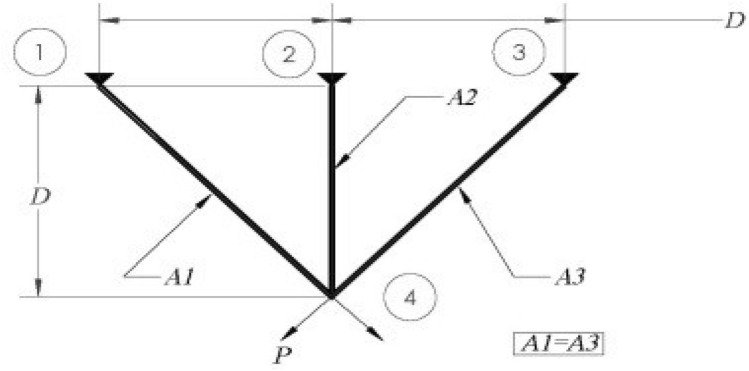
The proposed chaotic SMA method is applied for solving problem of truss design as shown in Fig. 12 [113, 114]. Truss design problem depends on two variables and three parameters. The main focus of truss design problem is to minimize weight. The various constraints involved in truss bar design problem are warping, deflection and stress. These constraints are optimized to achieve the desired objective. The mathematical modeling of 3-bar truss are illustrated through Eqs. (9.1) to (9.1d) subject to various constraints. The solutions of CSMA were compared with existing methods and illustrated in Table 20. It is seen that the suggested method appreciably improves the objective of cost minimization. The design problem is modeled as shown below:

Fig. 12.

Truss engineering design

Table 20.

Comparative analysis of CSMA results with other methods for 3-bar truss problem

Algorithm	CSMA	HHO [115]	MVO [6]	CS [116]	Ray and Sain [117]	TSA [118]
Variables
y1	0.763	0.78866	0.78860	0.7886	0.795	0.788
y2	0.494	0.40828	0.40845	0.409	0.395	0.408
Optimal weight	263.45	263.895	263.895	263.972	264.3	263.68

Consider,

$$\overrightarrow{y}=\left[y_1,y_2\right]=\left[A_1,A_2\right].$$ 9.1

Minimize,

$$f\left(\overrightarrow{y}\right)=\left(2\sqrt{2}{y}_1+y_2\right)\ast l.$$ 9.1a

Subjected to:

$$g_1\left(\overrightarrow{y}\right)=\frac{\sqrt{2}{y}_1+y_2}{\sqrt{2}{y}_1^2+2y_1{y}_2}P-\sigma \le 0$$ 9.1b

$$g_2\left(\overrightarrow{y}\right)=\frac{y_2}{\sqrt{2}{y}_1^2+2y_1{y}_2}P-\sigma \le 0$$ 9.1c

$$g_3\left(\overrightarrow{y}\right)=\frac{1}{\sqrt{2}{y}_2+y_1}P-\sigma \le 0.$$ 9.1d

Pressure vessel engineering problem

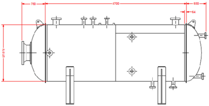
The design specification for this kind of engineering problem as illustrated in Fig. 13 [113, 114] is selected for reference. The chaotic SMA is applied to diminish the expense which includes the material cost and welding cost to form the vessel in cylindrical form. The four variables used to design the pressure vessel are: (i) shell thickness (T_s), (ii) head thickness (T_h), (iii) length of cylindrical unit (L_h), (iv) without head thickness (R). These four variables are modeled as y₁–y₄. The numerical formulation of this kind of problem is shown in Eqs. (9.2) through (9.2e). Table 21 shows the result assessment of suggested CSMA with some recent algorithms. From the comparative analysis, it is found that CSMA effectively reduces the expense of design by controlling the design variables:

Fig. 13.

Pressure vessel engineering design

Table 21.

Comparative analysis CSMA results with other methods

Algorithm	CSMA	GWO [119]	GSA [4]	PSO [120]	GA [121]	GA (Coello and Montes) [122]	GA (Deb and Gene) [122]	ES (Montes and Coello)	DE [123]	ACO [11]	Lagrangian multiplier [124]	Branch-bound [125]
Optimum value
Ts	0.778173	0.8125	1.125	0.8125	0.8125	0.8125	0.9375	0.8125	0.8125	0.8125	1.125	1.125
Th	0.3846	0.4345	0.625	0.4375	0.4345	0.4375	0.5	0.4375	0.4375	0.4375	0.625	0.625
R	40.3891	42.0892	55.9887	42.0913	40.3239	42.0974	48.329	42.0981	42.0984	42.1036	58.291	47.7
L	199.99	176.7587	84.4542	176.7465	200	176.6541	112.679	176.641	176.6377	176.5727	43.69	117.701
Optimum cost	5885.341	6051.564	8538.84	6061.078	6288.745	6059.946	6410.381	6059.75	6059.734	6059.089	7198.043	8129.1

Bold values indicate the results of the Chaotic variant of the Slime Mould Algorithm

Consider:

$$\overrightarrow{y}=\left[y_1{y}_2{y}_3{y}_4\right]=\left[T_{\text{s}}{T}_{\text{h}}R{L}_{\text{h}}\right].$$ 9.2

Minimize;

$$f(\overrightarrow{y})=0.6224y_1{y}_3{y}_4+1.7781y_2{y}_3^2+3.1661y_1^2{y}_4+19.84y_1^2{y}_3$$ 9.2a

Subject to:

$$g_1\left(\overrightarrow{y}\right)=-y_1+0.0193y_3\le 0$$ 9.2b

$$g_2\left(\overrightarrow{y}\right)=y_3+0.00954y_3\le 0$$ 9.2c

$$g_3\left(\overrightarrow{y}\right)=-\pi y_3^2{y}_4-\frac{4}{3}\pi y_3^3+1296000\le 0$$ 9.2d

$$g_4\left(\overrightarrow{y}\right)=y_4-240\le 0.$$ 9.2e

Variable range $0\le y_1\le 99$, $0\le y_2\le 99$, $10\le y_3\le 200$, $10\le y_4\le 200$, $0\le y_1\le 99$.

Compression spring engineering design

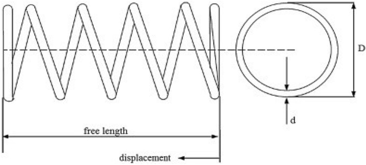
Compression spring design concerned with mechanical engineering [113, 114] is shown in Fig. 14. The main intention of this type of problem is minimization of the spring weight. There are three design variables: (1) no. of active coils (N_c), (2) wire diameter (d_r), and (3) mean coil diameter (D_m). The formulation is shown in the Eqs. (9.3) through (9.5f). The proposed method is applied to solve compression spring design problem and results are compared with other methods shown in Table 22 for validation. It is clearly seen from the analysis that CSMA method is efficient for reducing spring weight marginally.

Fig. 14.

Compression spring engineering design

Table 22.

Comparison of CSMA with other methods

Method	CSMA	GWO [15]	GSA [94]	CPSO [126]	ES [127]	GA [128]	HS [18]	DE [1]	MO [129]	CC [130]
Optimized value for variables
‘d’	0.05	0.0516	0.0503	0.0517	0.052	0.0515	0.0512	0.0516	0.0534	0.05
‘D’	0.3174	0.3567	0.3237	0.3576	0.364	0.3517	0.3499	0.3547	0.3992	0.3159
‘N’	14.0278	11.2889	13.5254	11.2445	10.8905	11.6322	12.0764	11.4108	9.1854	14.25
Optimum weight	0.012715	0.01267	0.0127	0.01267	0.01268	0.0127	0.01267	0.01267	0.01273	0.01283

Bold values indicate the results of the Chaotic variant of the Slime Mould Algorithm

Consider

$$\overrightarrow{y}=\left[y_1{y}_2{y}_3\right]=\left[d_{\text{r}}{D}_{\text{m}}{N}_{\text{c}}\right],$$ 9.3

Minimize

$$f(\overrightarrow{y})=\left(y_3+2\right)y_2{y}_1^2,$$ 9.3a

Subject to:

$$g_1\left(\overrightarrow{y}\right)=1-\frac{y_2^3{y}_3}{71785y_1^4}\le 0,$$ 9.3b

$$g_2\left(\overrightarrow{y}\right)=\frac{4y_2^2-y_1{y}_2}{12566\left(y_2{y}_1^3-y_1^4\right)}+\frac{1}{5108y_1^2}\le 0,$$ 9.3c

$$g_2\left(\overrightarrow{y}\right)=\frac{4y_2^2-y_1{y}_2}{12566\left(y_2{y}_1^3-y_1^4\right)}+\frac{1}{5108y_1^2}\le 0,$$ 9.3d

$$g_3\left(\overrightarrow{y}\right)=1-\frac{140.45y_1}{y_2^2{y}_3}\le 0,$$ 9.3e

$$g_4\left(\overrightarrow{y}\right)=\frac{y_1+y_2}{1.5}-1\le 0.$$ 9.3f

Variable range 0.005 ≤ $y_1$ ≤ 2.00, 0.25 ≤ $y_2$ ≤ 1.30, 2.00 ≤ $y_3$ ≤ 15.0.

Welded beam design

In welded beam design, welding is carried out by fusing different sections by molten metal as shown in Fig. 15 [113, 114]. The main focus is on minimization of the making cost of the welded beam. The four variables are: (1) bar thickness (b) is specified by y₁, (2) bar length (l) is specified by y₂, (3) weld thickness (h) is specified by y₃, and (4) the bar height (h) is specified by y₄ which is subject to constraints, such as Buckling of bar (P_c), side constraints, End deflection of beam (d), bending stress of the beam (h) and stress of shear (s). The equations of the above-mentioned design problem are noted by Eqs. (9.4) through (9.4n). The results are compared with other methods as shown in Table 23. The comparative analysis shows that proposed method is competent for handling beam design problem more precisely.

Fig. 15.

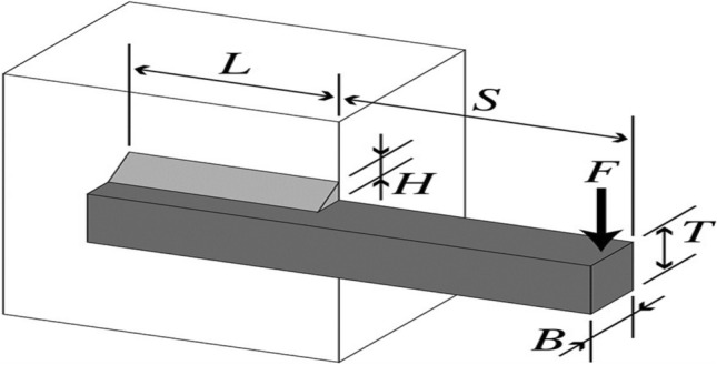
Welded beam engineering design

Table 23.

Comparative analysis of welded beam design with other methods

Method	CSMA	GSA [105]	GA1 [128]	GA2 [131]	HS [132]	Random [133]	Simplex [133]	David [133]	APPROX [133]
Optimum variables
h	0.2057	0.1821	0.24890	0.2088	0.2442	0.4575	0.2792	0.2434	0.2444
l	3.4710	3.857	6.17300	3.4205	6.2231	4.7313	5.6256	6.2552	6.2189
t	9.0366	10	8.1789	8.9975	8.2915	5.0853	7.7512	8.2915	8.2915
b	0.2057	0.2024	0.2533	0.2100	0.2443	0.66	0.2796	0.2444	0.2444
Optimal cost	1.7248	1.88	2.4334	1.7583	2.3807	4.1185	2.5307	2.3841	2.3815

Bold values indicate the results of the Chaotic variant of the Slime Mould Algorithm

Consider

$$\overrightarrow{y}=\left[y_1{y}_2{y}_3{y}_4\right]=\left[\mathit{hltb}\right].$$ 9.4

Minimize

$$f(\overrightarrow{y})=1.10471y_1^2{y}_2+0.04811y_3{y}_4\left(14.0+y_2\right)$$ 9.4a

Subject to

$$g_1(\overrightarrow{y})=\tau (\overrightarrow{y})-{\tau }_{\text{maxi}}\le 0,$$ 9.4b

$$g_2(\overrightarrow{y})=\sigma (\overrightarrow{y})-{\sigma }_{\text{maxi}}\le 0,$$ 9.4c

$$g_3(\overrightarrow{y})=\delta (\overrightarrow{y})-{\delta }_{\text{maxi}}\le 0,$$ 9.4d

$$g_4(\overrightarrow{y})=y_1-y_4\le 0,$$ 9.4e

$$g_5(\overrightarrow{y})=P_i-P_{\text{c}}(\overrightarrow{y})\le 0,$$ 9.4f

$$g_6(\overrightarrow{y})=0.125-y_1\le 0,$$ 9.4g

$$g_7(\overrightarrow{y})=1.10471y_1^2+0.04811y_3{y}_4(14.0+y_2)-5.0\le 0.$$ 9.4h

Variable range 0.1 ≤ $y_1$ ≤ 2, 0.1 ≤ $y_2$ ≤ 10, 0.1 ≤ $y_3$ ≤ 10, 0.1 ≤ $y_4$ ≤ 2,

where

$$\tau (\overrightarrow{y})=\sqrt{{({\tau }^{/})}^2+2{\tau }^{/}{\tau }^{//}\frac{y_2}{2R}+{({\tau }^{//})}^2,}$$ 9.4i

$${\tau }^{/}=\frac{P_i}{\sqrt{2}{y}_1{y}_2},{\tau }^{//}=\frac{\mathit{MR}}{J},M=P_i\left(L+\frac{y_2}{2}\right),$$ 9.4j

$$R=\sqrt{\frac{y_2^2}{4}+{\left(\frac{y_1+y_3}{2}\right)}^2},$$ 9.4k

$$J=2\left\{\sqrt{2}{y}_1{y}_2\left[\frac{y_2^2}{4}+{\left(\frac{y_1+y_3}{2}\right)}^2\right]\right\},$$ 9.4l

$$\sigma (\overrightarrow{y})=\frac{6P_{i}L}{y_4{y}_3^2},\delta (\overrightarrow{y})=\frac{6P_i{L}^3}{E{y}_2^2{y}_4},$$ 9.4m

$$P_{\text{c}}(\overrightarrow{y})=\frac{4.013E\frac{\sqrt{y_3^2{y}_4^6}}{36}}{L^2}\left(1,-,\frac{y_3}{2L},\sqrt{\frac{E}{4G}}\right)$$ 9.4n

$$\begin{array}{c}{P}_i=6000lb,L=14\text{in},{\delta }_{maxi}=0.25\text{in},E=30\times 1^6\text{psi},G=12\times {10}^6\text{psi},\\ {\tau }_{\text{maxi}}=13600\text{psi},{\sigma }_{\text{maxi}}=3000\text{psi}.\\ \end{array}$$

Cantilever beam design

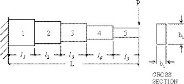
This is civil engineering problem in which main focus is minimization of beam weight as shown in Fig. 16. In beam design, there are five elements $l_1,l_2,l_3,l_4\text{and}{l}_5$ [114]. The main aim is minimization of the weight of the beam shown in Eq. (9.5). Taking care that displacement of vertical constraint not to disturb during finishing process of the beam for final optimal solution shown by Eq. (9.5a) to Eq. (9.5b). The results shown in Table 24 validate that CSMA algorithm efficiently reduces the weight of the beam. The formulation of design is given below:

Fig. 16.

Cantilever beam engineering design

Table 24.

Comparative analysis of beam problem with other methods

Method	CSMA	ALO [134]	SOS [28]	CS [135]	MMA [136]	GCA_I [136]	GCA_II [136]
Optimal values for variables
l1	5.9700	6.0181	6.0188	6.0089	6.01	6.01	6.01
l2	4.8841	5.3114	5.3034	5.3049	5.3	5.304	5.3
l3	4.4544	4.4884	4.4959	4.5023	4.49	4.49	4.49
l4	3.4738	3.4975	3.499	3.5077	3.49	3.498	3.49
l5	2.1571	2.1583	2.1556	2.1504	2.15	2.15	2.15
Optimum weight	1.30328	1.3399	1.33996	1.33999	1.34	1.34	1.34

Bold values indicate the results of the Chaotic variant of the Slime Mould Algorithm

Consider

$$\overrightarrow{x}=\left[l_1{l}_2{l}_3{l}_4{l}_5\right].$$ 9.5

Minimize

$$\begin{array}{c}f(\overrightarrow{x})=0.6224(l_1+l_2+l_3+l_4+l_5),\\ \\ \end{array}$$ 9.5a

Subject to

$$g(\overrightarrow{x})=\frac{61}{l_1^3}+\frac{37}{l_2^3}+\frac{19}{l_3^3}+\frac{7}{l_4^3}+\frac{1}{l_5^3}\le 1.$$ 9.5b

Gear train design

In this method, the four variables $g_1,g_2,g_3,\text{and}{g}_4$ are reformed to diminish the scalar value and teeth ratio as shown in Fig. 17 [113]. Teeth on each gear are the decision variables in designing process. The gear train design problem is formulated through Eq. (9.6a) to Eq. (9.6b). The simulation results shown in Table 25 reveal that CSMA method gives comparison of results with other methods. From the assessment of test results, it is seen that proposed method effectively evaluates the gear train ratio.

Fig. 17.

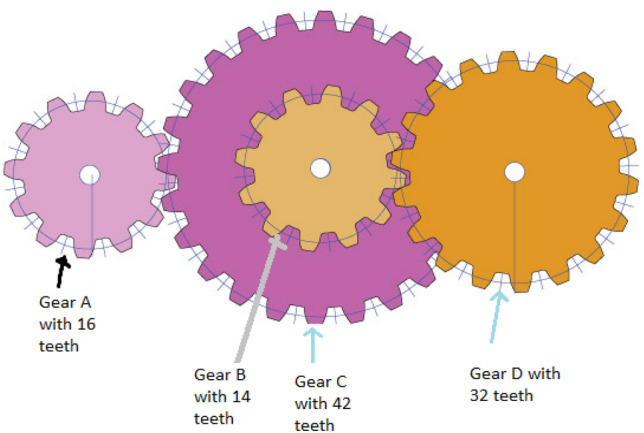
Gear train problem

Table 25.

Comparison of gear train problem with other methods

Method	CSMA	Gene AS [121]	Kannan and Kramer [121]	Sandgren [121]
Optimal values for variables
x1	41	50	41	60
x2	33	33	33	45
x3	15	14	15	22
x4	13	17	13	18
Optimum fitness	0.144124	0.144124	0.144124	0.146667

Let us consider:

$$\overrightarrow{g}=\left[g_1{g}_2{g}_3{g}_4\right]=\left[M_A{M}_B{M}_C{M}_D\right]$$ 9.6a

Minimizing

$$f(\overrightarrow{g})={\left(\frac{1}{6.931}-\frac{g_3{g}_4}{g_1{g}_4}\right)}^2.$$ 9.6b

Subject to: $12\le g_1,g_2,g_3,g_4\le 60$.

Speed reducer engineering design problem

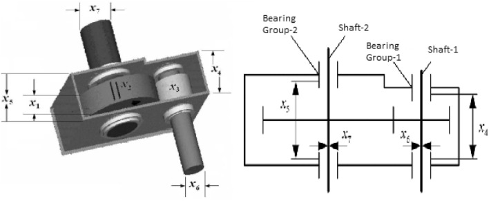
The fundamental problem is to limit the heaviness of the speed reducer. This type of design problem consist of seven variables as shown in Fig. 18 [113]. The seven variables are face width $(x_1)$, teeth module $(x_2)$, pinion teeth $(x_3)$, first shaft length $(x_4)$, second shaft length $(x_5)$, the first shaft diameter $(x_6)$ and second shaft diameter $(x_7)$. The results shown in Table 26 shows that optimum fitness has been improved to some extend from previous evaluation. The equations are formulated as given below:

Fig. 18.

Speed reducer engineering design problem

Table 26.

Comparison of speed reducer problem with other methods

Method	CSMA	HEAA [137]	MDE [138]	PSO-DE [139]	MBA [113]
Optimal values for variables
x1	3.5	3.500022	3.50001	3.50	3.5
x2	0.7	0.70000039	0.7	0.7	0.7
x3	17	17.000012	17	17	17
x4	7.3	7.300427	7.300156	7.3	7.300033
x5	7.715418	7.715377	7.800027	7.8	7.715772
x6	3.350215	3.35023	3.350221	3.350214	3.350218
x7	5.286655	5.286663	5.286685	5.286683	5.286654
Optimum fitness	2994.4737	2994.49911	2996.35669	2996.3481	2994.4824

Bold values indicate the results of the Chaotic variant of the Slime Mould Algorithm

Minimizing

$$\begin{array}{cc}\hfill f(\overrightarrow{x})& =0.7854x_1{x}_2(3.3333x_3^2+14.9334x_3-43.0934)-1.508x_1(x_6^2+x_7^2)+7.4777(x_6^3+x_7^3)\hfill \\ \hfill & +0.7854(x_4{x}_6^2+x_5{x}_7^2)\hfill \\ \hfill \end{array}$$

Subject to:

$$g_1(\overrightarrow{x})=\frac{27}{x_1{x}_2^2{x}_3}-1\le 0$$ 9.7a

$$g_2(\overrightarrow{x})=\frac{397.5}{x_1{x}_2^2{x}_3^2}-1\le 0$$ 9.7b

$$g_3(\overrightarrow{x})=\frac{1.93x_4^3}{x_2{x}_3{x}_6^4}-1\le 0$$ 9.7c

$$g_4(\overrightarrow{x})=\frac{1.93x_5^3}{x_2{x}_3{x}_7^4}-1\le 0$$ 9.7d

$$g_5(\overrightarrow{x})=\frac{1}{110x_6^3}{\sqrt{\left(\frac{745.0x_4}{x_2{x}_3}\right)}}^2+16.9\times {10}^6-1\le 0$$ 9.7e

$$g_6(\overrightarrow{x})=\frac{1}{85x_7^3}{\sqrt{\left(\frac{745.0x_5}{x_2{x}_3}\right)}}^2+157.5\times {10}^6-1\le 0$$ 9.7f

$$g_7(\overrightarrow{x})=\frac{x_2{x}_3}{40}-1\le 0$$ 9.7g

$$g_8(\overrightarrow{x})=\frac{5x_2}{x_1}-1\le 0$$ 9.7h

$$g_9(\overrightarrow{x})=\frac{x_1}{12x_2}-1\le 0$$ 9.7i

$$g_{10}(\overrightarrow{x})=\frac{1.5x_6+1.9}{12x_2}-1\le 0$$ 9.7j

$$g_{11}(\overrightarrow{x})=\frac{1.1x_7+1.9}{x_5}-1\le 0$$ 9.7k

where $2.6\le x_1\le 3.6,0.7\le x_2\le 0.8,17\le x_3\le 28,7.3\le x_4\le 8.3,7.8\le x_5\le 8.3,2.9\le x_6\le 3.9\text{and}5\le x_7\le 5.5.$

Belleville spring design

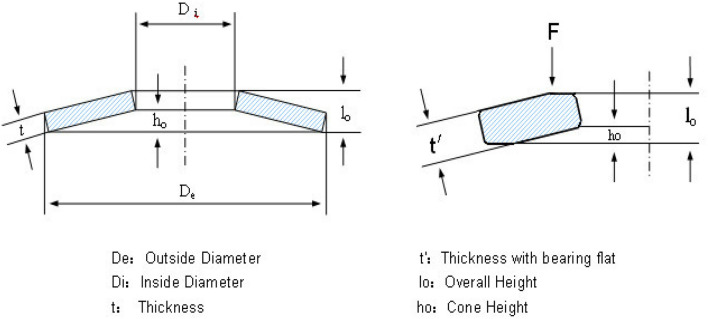
This type of design problem is shown in Fig. 19 [113]. In this method, one of the design parameter is selected according to variable ratio. The focus of this method is to minimize weight within certain constraints. The designed variables are internal diameter of the spring (DIMI), external diameter of the spring (DIME), spring height (SH) and spring thickness (ST). The results are compared with other methods as shown in Table 27. The assessment of CHHO with other methods reveals that present method is effective in solving spring design problem more precisely. The mathematical formulation for spring design are given below:

Fig. 19.

Belleville spring engineering design

Table 27.

Comparative analysis of Belleville spring design variables with other methods

Method	CSMA	TLBO [9]	MBA [113]
Values for variables
x1	8.83686	12.01	12.01
x2	4.81595	10.0304	10.0304
x3	0.2	0.20414	0.20414
x4	0.2	0.2	0.2
Optimum fitness	0.0572	0.19896	0.19896

Bold values indicate the results of the Chaotic variant of the Slime Mould Algorithm

Minimizing

$$f(x)=0.07075\pi ({\text{DIM}}_{\text{E}}^2-{\text{DIM}}_{\text{I}}^2)t$$ 9.8a

Subject to:

$$b_1(x)=G-\frac{4P{\lambda }_{max}}{(1-{\delta }^2)\alpha {\text{DIM}}_{\text{E}}}\left[\delta (S_{\text{H}}-\frac{\lambda max}{2})+\mu t\right]\ge 0$$ 9.8b

$$b_2(x)={\left(\frac{4P{\lambda }_{max}}{(1-{\delta }^2)\alpha {\text{DIM}}_{\text{E}}}\left[\left(S_{\text{H}}-\frac{\lambda }{2}\right)(S_{\text{H}}-\lambda )t+t^3\right]\right)}_{{\lambda }_{max}}-P_{\text{MAX}}\ge 0$$ 9.8c

$$b_3(x)={\lambda }_1-{\lambda }_{max}\ge 0$$ 9.8d

$$b_4(x)=H-S_{\text{H}}-t\ge 0$$ 9.8e

$$b_5(x)={\text{DIM}}_{\text{MAX}}-{\text{DIM}}_{\text{E}}\ge 0$$ 9.8f

$$b_6(x)={\text{DIM}}_{\text{E}}-{\text{DIM}}_{\text{I}}\ge 0$$ 9.8g

$$b_7(x)=0.3-\frac{S_{\text{H}}}{{\text{DIM}}_{\text{E}}-{\text{DIM}}_{\text{I}}}\ge 0$$ 9.8h

where $\alpha =\frac{6}{\pi lnJ}{\left(\frac{J-1}{J}\right)}^2$

$$\delta =\frac{6}{\pi lnJ}\left(\frac{J-1}{lnJ}-1\right)$$

$$\mu =\frac{6}{\pi lnJ}\left(\frac{J-1}{2}\right)$$

$$P_{\text{MAX}}=5400lb$$

$$\begin{array}{c}P=30e6\text{psi},{\lambda }_{max}=0.2\text{in},\delta =0.3,G=200\text{Kpsi},\\ H=2\text{in},{\text{DIM}}_{\text{MAX}}=12.01\text{in},J=\frac{{\text{DIM}}_{\text{E}}}{{\text{DIM}}_{\text{I}}},{\lambda }_1=f(a)a,a=\frac{S_{\text{H}}}{t}.\\ \end{array}$$

Rolling element bearing design

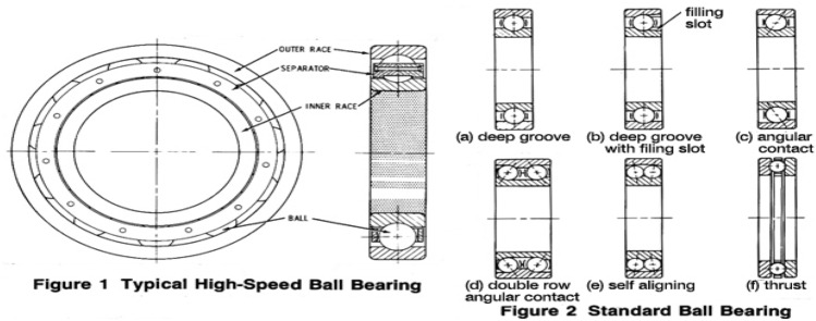
The major aspect of this kind of design is to improve the dynamic load carrying capacity of rolling bearing element as illustrated in Fig. 20 [89]. There are ten parameters which decides the optimum design of bearing for improving the load bearing power. Out of these ten variables only five variables are of much consideration. These major variables are (1) diameter of the ball (DIMB), (2) diameter pitch (DIMP), (3) ball numbers (N_b), (4) outer curvature coefficient and (5) inner curvature coefficient. Rest of five variables only affect indirectly to the internal portion of the geometry. The proposed algorithm is applied to solve rolling design problem and outputs are compared with other methods as illustrated in Table 28. From the result assessment, it can be seen that CSMA gives analogous outcomes. The design equations are formulated through the following equations:

Fig. 20.

Rolling element bearing problem

Table 28.

Comparative analysis of rolling element design variables

Method	CSMA	WCA [140]	SCA [141]	MFO [16]	MVO [142]
Values for variables
r1	125.7227	125.72	125	125	125.6002
r2	21.4233	21.42300	21.03287	21.03287	21.32250
r3	11.00116	10.01030	10.96571	10.96571	10.97338
r4	0.515	0.515000	0.515	0.515	0.515
r5	0.515	0.515000	0.515	0.515000	0.515000
r6	0.4944	0.401514	0.5	0.5	0.5
r7	0.6986	0.659047	0.7	0.67584	0.68782
r8	0.3	0.300032	0.3	0.300214	0.301348
r9	0.03346	0.040045	0.027780	0.02397	0.03617
r10	0.60049	0.600000	0.62912	0.61001	0.61061
Optimum fitness	− 85,534.166	85,538.48	83,431.11	84,002.524	84,491.266

Bold values indicate the results of the Chaotic variant of the Slime Mould Algorithm

Maximizing

$$C_{\text{D}}=f_{\text{c}}{N}^{2/3}{\text{DIM}}_{\text{B}}^{1.8}$$ 9.9a

$$\text{if}\text{DIM}\le 25.4\text{mm}$$

$$C_{\text{D}}=3.647f_{\text{c}}{N}^{2/3}{\text{DIM}}_{\text{B}}^{1.4}$$ 9.9b

$$\text{if}\text{DIM}\ge 25.4\text{mm}$$

Subjected to:

$$r_1(x)=\frac{{\theta }_0}{2{sin}^{-1}\left(\frac{{\text{DIM}}_{\text{B}}}{{\text{DIM}}_{\text{MAX}}}\right)}-N+1\ge 0$$ 9.9c

$$r_2(x)=2{\text{DIM}}_{\text{B}}-K_{{\text{DIM}}_{\text{MIN}}}(\text{DIM}-dim)\ge 0$$ 9.9d

$$r_3(x)=K_{{\text{DIM}}_{\text{MAX}}}(\text{DIM}-dim)\ge 0$$ 9.9e

$$r_4(x)=\beta B_W-{\text{DIM}}_{\text{B}}\le 0$$ 9.9f

$$r_4(x)={\text{DIM}}_{\text{MAX}}-0.5(\text{DIM}+dim)\ge 0$$ 9.9g

$$r_5(x)={\text{DIM}}_{\text{MAX}}-0.5(\text{DIM}+dim)\ge 0$$ 9.9h

$$r_6(x)=(0.5+\text{re})(\text{DIM}+dim)\ge 0$$ 9.9i

$$r_7(x)=0.5(\text{DIM}-{\text{DIM}}_{\text{MAX}}-{\text{DIM}}_{\text{B}})-\alpha {\text{DIM}}_{\text{B}}\ge 0$$ 9.9j

$$r_8(x)=f_I\ge 0.515$$ 9.9k

$$r_9(x)=f_0\ge 0.515,$$ 9.9l

where

$$f_{\text{c}}=37.91{\left[1+{\left\{1.04{\left(\frac{1-\epsilon }{1+\epsilon }\right)}^{1.72}{\left(\frac{f_{\text{I}}\left(2f_0-1\right)}{f_0\left(2f_{\text{I}}-1\right)}\right)}^{0.41}\right\}}^{10/3}\right]}^{-0.3}\times \left[\frac{{\epsilon }^{0.3}{\left(1-\epsilon \right)}^{1.39}}{{\left(1+\epsilon \right)}^{1/3}}\right]{\left[\frac{2f_{\text{I}}}{2f_{\text{I}}-1}\right]}^{0.41}$$

$${\theta }_0=2\pi -2{cos}^{-1}\left(\frac{\left[{\left\{(\text{DIM}-dim)/2-3(t/4)\right\}}^2+{\left(\text{DIM}/2-t/4-{\text{DIM}}_{\text{B}}\right)}^2-{\left\{dim/2+t/4\right\}}^2\right]}{2\left\{(\text{DIM}-dim)/2-3(t/4)\right\}\left\{D/2-t/4-{\text{DIM}}_{\text{B}}\right\}}\right)$$

$$\epsilon =\frac{{\text{DIM}}_{\text{B}}}{{\text{DIM}}_{\text{MAX}}},f_{\text{I}}=\frac{R_{\text{I}}}{{\text{DIM}}_{\text{B}}},f_0=\frac{R_0}{{\text{DIM}}_{\text{B}}},t=\text{DIM}-dim-2{\text{DIM}}_{\text{B}}$$

$$\text{DIM}=160,dim=90,B_W=30,R_{\text{I}}=R_0=11.033$$

$\begin{array}{c}0.5\left(\text{DIM}+dim\right)\le {\text{DIM}}_{\text{MAX}}\le 0.6\left(\text{DIM}+dim\right),0.15\left(\text{DIM}-dim\right)\le {\text{DIM}}_{\text{B}}\le 0.45\left(\text{DIM}-dim\right),4\le N\le 50\\ 0.515\le f_{\text{I}}\text{and}{f}_0\le 0.6\\ 0.4\le K_{{\text{DIM}}_{\text{MIN}}}\le 0.5,0.6\le K_{{\text{DIM}}_{\text{MIN}}}\le 0.7,0.3\le \text{re}\le 0.1,0.02\le \text{re}\le 0.1,0.6\le \beta \le 0.85.\\ \end{array}$

Multidisc-clutch design

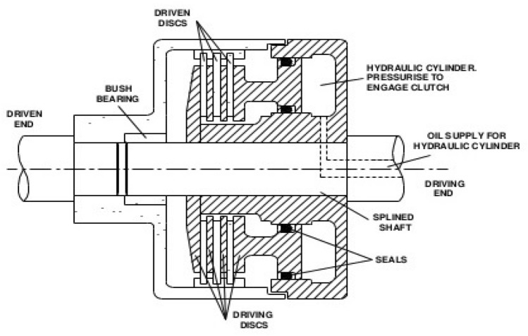
Brake design is one of the most crucial problem in engineering and is shown in Fig. 21 [143]. The clutch-design problem is mainly fabricated to minimize the overall weight. The five design variables are inner surface radius (R_in), outer surface radius (R_o), thickness of disc’s (Th), actuating force (Fac) and count of friction surface (S_f). In Table 29, results are compared and observed that optimum fitness is found to better than other methods. The equations for Multidisc brake problem are given below:

Fig. 21.

Multidisc clutch break design

Table 29.

Comparative analysis of multiple-disc clutch brake problem with other methods

Method	CSMA	NSGA-II	TLBO [9]	AM-DE [138]
Best values for variables
x1	69.99	70	70	70.00
x2	90	90	90	90
x3	2.312	3	3	3
x4	1.5	1.5	1	1
x5	1000	1000	810	810
Optimum fitness	0.38965	0.4704	0.31365	0.3136566

Bold values indicate the results of the Chaotic variant of the Slime Mould Algorithm

Minimizing

$$f\left(R_{\text{in}},R_{\text{o}},S_{\text{f}},\text{Th}\right)=\pi \text{Th}\gamma \left(R_0^2-R_{\text{in}}^2\right)\left(S_{\text{f}}+1\right)$$ 9.10a

where $R_{\text{in}}\in 60,61,62\dots 80;R_{\text{o}}\in 90,91,\dots 110;\text{Th}\in 1,1.5,2,2.5,3;F_{\text{ac}}\in 600,610,620,1000;S_{\text{f}}\in 2,3,4,5,6,7,8,9.$

Subject to:

$$m_1=R_0-R_{\text{in}}-\mathrm{\Delta }R\ge 0$$ 9.10b

$$m_2=L_{\text{MAX}}-(S_{\text{f}}+1)(\text{Th}+\alpha )\ge 0$$ 9.10c

$$m_3={\text{PM}}_{\text{MAX}}-{\text{PM}}_{\pi }\ge 0$$ 9.10d

$$m_4={\text{PM}}_{\text{MAX}}{Y}_{\text{MAX}}+{\text{PM}}_{\pi }{Y}_{\text{SR}}\ge 0$$ 9.10e

$$m_5=Y_{{\text{SR}}_{\text{MAX}}}-Y_{\text{SR}}\ge 0$$ 9.10f

$$m_6=t_{\text{MAX}}-t\ge 0$$ 9.10g

$$m_7={\text{DC}}_{\text{h}}-{\text{DC}}_{\text{f}}\ge 0$$ 9.10h

$$m_8=t\ge 0$$ 9.10i

where

${\text{PM}}_{\pi }=\frac{F_{\text{ac}}}{\mathrm{\Pi }\left(R_0^2-R_{\text{in}}^2\right)}$

$$Y_{\text{SR}}=\frac{2\pi n\left(R_0^3-R_{\text{in}}^3\right)}{90\left(R_0^2-R_{\text{in}}^2\right)}$$

$$t=\frac{i_x\pi n}{30\left({\text{DC}}_{\text{h}}+{\text{DC}}_{\text{f}}\right)}$$

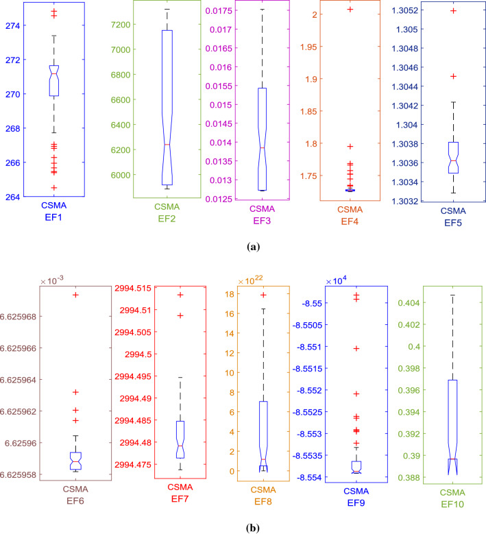
To check the effectiveness of chaotic SMA, algorithm is tested for 30 trial runs. The algorithm is tested with respect for best value, worst value, p value and standard deviation along with the trial runs. Furthermore, a comparative analysis with recent optimization methods is provided for justifying the validity of tested results for each of the standard function’s and design problems. Figure 22a and b shows 30 trial runs and for 10 multidisciplinary engineering problems to check the optimality of the algorithm.

Fig. 22.

Trial run test for engineering design problems

Conclusion

In the proposed research, the exploitation phase of the classical SMA has been enhanced by incorporating sinusoidal chaotic function. The resultant chaotic SMA has been applied to 23 standard benchmark problems. In the set of experiments, CSMA was compared with basic SMA. The test results of benchmark functions are also compared with other algorithms in terms of mean and standard deviation. To check the soundness of the proposed algorithm, results of CSMA has been compared with others recently developed and well-known classical optimizers such as PSO, DE, SSA, MVO, GWO, DE, MFO, SCA, CS, TSA, PSO-DE, GA, HS, Ray and Sain, MBA, ACO, and MMA. Experimental results suggest that chaotic strategy enables SMA to improve the exploitation phase with better convergence. Simulation results shows that the developed chaotic SMA algorithm outperforms on almost all benchmark functions. Furthermore, the CSMA is applied to solve 10 real-world engineering design problems. Each design problem with a specific objective function has been simulated by implementing CSMA. Engineering design problems are mostly analyzed in terms of weight minimization and reduced manufacturing cost. The comparative analysis reveals that the proposed method effectively explores the search space to optimize objective fitness and proofs that CSMA can demonstrate good results not only on unrestricted issues but also on restricted issues. It is seen that the resultant chaotic slime mold algorithm is capable of giving more optimistic and convergent results. Thus, the proposed CSMA may be a good choice for solving numerical optimization problems.

Limitation and future scope

The proposed optimizer is giving a powerful and optimal solution depending on the type of chaotic strategy opted, if chaotic strategies are not properly decided, it may lead to insignificant results also. Therefore, it is recommended that proper selection of chaotic strategy is required for significant results, so that the exploitation phase of the existing algorithm can be explored in a most significant way. In the future, the proposed chaotic variant may be significantly used to solve the various engineering and design optimization problems including power system optimization problems such as Economic Load Dispatch, Generation Scheduling problem, Unit commitment problem, and Automatic generation control and load frequency issues of realistic power system and in more deeper sense, it may be applied to solve power system dispatch and unit commitment problems considering electric and hybrid electric vehicles including uncertainty of wind and solar power.

References

- 1.Storn R, Price K. Differential evolution-a simple and efficient heuristic for global optimization over continuous spaces. J Glob Optim. 1997;11:341–359. doi: 10.1023/A:1008202821328. [DOI] [Google Scholar]
- 2.Koza JR, Poli R. Search methodologies. Boston, MA: Springer; 2005. Genetic programming; pp. 127–164. [Google Scholar]
- 3.Qin AK, Huang VL, Suganthan PN. Differential evolution algorithm with strategy adaptation for global numerical optimization. IEEE Trans Evol Comput. 2009;13:398–417. doi: 10.1109/TEVC.2008.927706. [DOI] [Google Scholar]
- 4.Rashedi E, Nezamabadi-Pour H, Saryazdi S. GSA: a gravitational search algorithm. Inf Sci. 2009;179:2232. doi: 10.1016/j.ins.2009.03.004. [DOI] [Google Scholar]
- 5.Kaveh Ali. Advances in metaheuristic algorithms for optimal design of structures. Switzerland: Springer International Publishing; 2014. [Google Scholar]
- 6.Mirjalili S, Mirjalili SM, Hatamlou A. Multi-verse optimizer: a nature-inspired algorithm for global optimization. Neural Comput Appl. 2016;27:495–513. doi: 10.1007/s00521-015-1870-7. [DOI] [Google Scholar]
- 7.Moghdani R, Salimifard K. Volleyball premier league algorithm. Appl Soft Comput J. 2018;64:161–185. doi: 10.1016/j.asoc.2017.11.043. [DOI] [Google Scholar]
- 8.Glover F. Tabu search—part I.ORSA. J Comput. 1989;1(3):190–206. [Google Scholar]
- 9.Satapathy SC, Naik A, Parvathi K. A teaching learning based optimization based on orthogonal design for solving global optimization problems. Springerplus. 2013;2:1–12. doi: 10.1186/2193-1801-2-130. [DOI] [PMC free article] [PubMed] [Google Scholar]
- 10.Eberhart R, Kennedy J (1995) Particle swarm optimization. In: Proceedings of the IEEE international conference on neural networks, vol. 4
- 11.Dorigo M, Birattari M, Stutzle T. Ant colony optimization. IEEE Comput Intell Mag. 2006;1:28–39. doi: 10.1109/MCI.2006.329691. [DOI] [Google Scholar]
- 12.Brajevic I, Tuba M. An upgraded artificial bee colony (ABC) algorithm for constrained optimization problems. J Intell Manuf. 2013;24:729–740. doi: 10.1007/s10845-011-0621-6. [DOI] [Google Scholar]
- 13.Verma C, Stoffova V, Illes Z, Tanwar S, Kumar N. Machine learning-based student’s native place identification for real-time. IEEE Access. 2020;8:130840–130854. doi: 10.1109/ACCESS.2020.3008830. [DOI] [Google Scholar]
- 14.Yang XS. Bat algorithm for multi-objective optimisation. Int J Bioinspired Comput. 2011;3:267–274. doi: 10.1504/IJBIC.2011.042259. [DOI] [Google Scholar]
- 15.Mirjalili S, Mirjalili SM, Lewis A. Grey wolf optimizer. Adv Eng Softw. 2014;69:46–61. doi: 10.1016/j.advengsoft.2013.12.007. [DOI] [Google Scholar]
- 16.Mirjalili S. Moth-flame optimization algorithm: a novel nature-inspired heuristic paradigm. Knowl Based Syst. 2015;89:228–249. doi: 10.1016/j.knosys.2015.07.006. [DOI] [Google Scholar]
- 17.Verma C, Stoffová V, Illés Z. Prediction of students’ awareness level towards ICT and mobile technology in Indian and Hungarian University for the real-time: preliminary results. Heliyon. 2019 doi: 10.1016/j.heliyon.2019.e01806. [DOI] [PMC free article] [PubMed] [Google Scholar]
- 18.Heidari AA, Mirjalili S, Faris H, Aljarah I, Mafarja M, Chen H. Harris hawks optimization: algorithm and applications. Future Gener Comput Syst. 2019 doi: 10.1016/j.future.2019.02.028. [DOI] [Google Scholar]
- 19.Verma C, Stoffová V, Illés Z. An Ensemble approach to identifying the student gender towards information and communication technology awareness in European schools using machine learning. Int J Eng Technol. 2018;7:3392–3396. doi: 10.14419/ijet.v7i4.14045. [DOI] [Google Scholar]
- 20.Fleszar K, Osman IH, Hindi KS. A variable neighbourhood search algorithm for the open vehicle routing problem. Eur J Oper Res. 2009;195:803–809. doi: 10.1016/j.ejor.2007.06.064. [DOI] [Google Scholar]
- 21.Simon D. Biogeography-based optimization. IEEE Trans Evol Comput. 2008;12:702–713. doi: 10.1109/TEVC.2008.919004. [DOI] [Google Scholar]
- 22.Tan Y, Zhu Y (2010) Fireworks algorithm for optimization. In: International conference in swarm intelligence. Springer, Berlin, Heidelberg
- 23.Gandomi AH, Alavi AH. Krill herd: a new bio-inspired optimization algorithm. Commun Nonlinear Sci Numer Simul. 2012;17:4831–4845. doi: 10.1016/j.cnsns.2012.05.010. [DOI] [Google Scholar]
- 24.Martí R, Resende MGC, Ribeiro CC. Multi-start methods for combinatorial optimization. Eur J Oper Res. 2013;226:1–8. doi: 10.1016/j.ejor.2012.10.012. [DOI] [Google Scholar]
- 25.Eskandar H, Sadollah A, Bahreininejad A, Hamdi M. Water cycle algorithm—a novel metaheuristic optimization method for solving constrained engineering optimization problems. Comput Struct. 2012;110–111:151–166. doi: 10.1016/j.compstruc.2012.07.010. [DOI] [Google Scholar]
- 26.Li X, Zhang J, Yin M. Animal migration optimization: An optimization algorithm inspired by animal migration behavior. Neural Comput Appl. 2014;24:1867–1877. doi: 10.1007/s00521-013-1433-8. [DOI] [Google Scholar]
- 27.Kuo HC, Lin CH. Cultural evolution algorithm for global optimizations and its applications. J Appl Res Technol. 2013;11:510–522. doi: 10.1016/S1665-6423(13)71558-X. [DOI] [Google Scholar]
- 28.Cheng MY, Prayogo D. Symbiotic organisms search: a new metaheuristic optimization algorithm. Comput Struct. 2014;139:98–112. doi: 10.1016/j.compstruc.2014.03.007. [DOI] [Google Scholar]
- 29.Gandomi AH. Interior search algorithm (ISA): a novel approach for global optimization. ISA Trans. 2014;53:1168–1183. doi: 10.1016/j.isatra.2014.03.018. [DOI] [PubMed] [Google Scholar]
- 30.Mirjalili S, Wang GG, Coelho LS. Binary optimization using hybrid particle swarm optimization and gravitational search algorithm. Neural Comput Appl. 2014;25:1423–1435. doi: 10.1007/s00521-014-1629-6. [DOI] [Google Scholar]
- 31.Mohseni S, et al. (2014) Competition over resources: a new optimization algorithm based on animals behavioral ecology. In: 2014 International Conference on Intelligent Networking and Collaborative Systems. IEEE
- 32.Wang GG, Guo L, Gandomi AH, Hao GS, Wang H. Chaotic Krill Herd algorithm. Inf Sci (Ny) 2014;274:17–34. doi: 10.1016/j.ins.2014.02.123. [DOI] [Google Scholar]
- 33.Salimi H. Stochastic fractal search: a powerful metaheuristic algorithm. Knowl Based Syst. 2015;75:1–18. doi: 10.1016/j.knosys.2014.07.025. [DOI] [Google Scholar]
- 34.Ghorbani N, Babaei E. Exchange market algorithm. Appl Soft Comput J. 2014;19:177–187. doi: 10.1016/j.asoc.2014.02.006. [DOI] [Google Scholar]
- 35.Ghaemi M, Feizi-Derakhshi MR. Forest optimization algorithm. Expert Syst Appl. 2014;41:6676–6687. doi: 10.1016/j.eswa.2014.05.009. [DOI] [Google Scholar]
- 36.Gray B, Optimization W. Author’s accepted manuscript binary gray wolf optimization approaches for feature selection. Neurocomputing. 2015 doi: 10.1016/j.neucom.2015.06.083. [DOI] [Google Scholar]
- 37.Meng XB, Gao XZ, Lu L, Liu Y, Zhang H. A new bio-inspired optimisation algorithm: Bird Swarm Algorithm. J Exp Theor Artif Intell. 2016;28:673–687. doi: 10.1080/0952813X.2015.1042530. [DOI] [Google Scholar]
- 38.Wang GG, Suash D, Coelho LDS (2015) Elephant herding optimization. In: 2015 3rd International Symposium on Computational and Business Intelligence (ISCBI). IEEE
- 39.Abedinpourshotorban H, Mariyam Shamsuddin S, Beheshti Z, Jawawi DNA. Electromagnetic field optimization: a physics-inspired metaheuristic optimization algorithm. Swarm Evol Comput. 2016;26:8–22. doi: 10.1016/j.swevo.2015.07.002. [DOI] [Google Scholar]
- 40.Shahriar MS, Rana J, Asif MA, Hasan M, Hawlader M (2015) Optimization of Unit Commitment Problem for wind-thermal generation using Fuzzy optimization technique. In: 2015 International conference on advances in electrical engineering (ICAEE), pp. 88–92. IEEE
- 41.Shareef H, Ibrahim AA, Mutlag AH. Lightning search algorithm. Appl Soft Comput J. 2015;36:315–333. doi: 10.1016/j.asoc.2015.07.028. [DOI] [Google Scholar]
- 42.Saremi S, Mirjalili S, Lewis A. Grasshopper optimisation algorithm: theory and application. Adv Eng Softw. 2017;105:30–47. doi: 10.1016/j.advengsoft.2017.01.004. [DOI] [Google Scholar]
- 43.Singh N, Singh SB. A novel hybrid GWO-SCA approach for optimization problems. Eng Sci Technol Int J. 2017;20:1586–1601. doi: 10.1016/j.jestch.2017.11.001. [DOI] [Google Scholar]
- 44.Gohil NB, Dwivedi VV. A review on lion optimization. Nat Inspired Evol Algorithm. 2017;7:340–352. [Google Scholar]
- 45.Reddy SK, Panwar L, Panigrahi BK, Kumar R. Binary whale optimization algorithm: a new metaheuristic approach for profit-based unit commitment problems in competitive electricity markets. Eng Optim. 2018 doi: 10.1080/0305215X.2018.1463527. [DOI] [Google Scholar]
- 46.Pierezan J, Coelho LDS (2018) Coyote optimization algorithm: a new metaheuristic for global optimization problems. In: 2018 IEEE congress on evolutionary computation (CEC). IEEE
- 47.Chen X, Tianfield H, Li K. BASE DATA. Swarm Evol Comput. 2019 doi: 10.1016/j.swevo.2019.01.003. [DOI] [Google Scholar]
- 48.Shadravan S, Naji HR, Bardsiri VK. The Sailfish Optimizer: a novel nature-inspired metaheuristic algorithm for solving constrained engineering optimization problems. Eng Appl Artif Intell. 2019;80:20–34. doi: 10.1016/j.engappai.2019.01.001. [DOI] [Google Scholar]
- 49.Verma C, Illes Z, Stoffova V (2019) Age group predictive models for the real time prediction of the university students using machine learning: Preliminary results. In: 2019 IEEE International Conference on Electrical, Computer and Communication Technologies (ICECCT). IEEE
- 50.Adamatzky A. Slime mold solves maze in one pass, assisted by gradient of chemo-attractants. IEEE Trans Nanobiosci. 2012;11:131–134. doi: 10.1109/TNB.2011.2181978. [DOI] [PubMed] [Google Scholar]
- 51.Nakagaki T, Kobayashi R, Nishiura Y, Ueda T. Obtaining multiple separate food sources: behavioural intelligence in the Physarum plasmodium. Proc R Soc B Biol Sci. 2004;271:2305–2310. doi: 10.1098/rspb.2004.2856. [DOI] [PMC free article] [PubMed] [Google Scholar]
- 52.Adamatzky A, Jones J. Road planning with slime mould: if Physarum built motorways it would route M6/M74 through Newcastle. Int J Bifurc Chaos. 2010;20:3065–3084. doi: 10.1142/S0218127410027568. [DOI] [Google Scholar]
- 53.Beekman M, Latty T. Brainless but multi-headed: decision making by the acellular slime mould Physarum polycephalum. J Mol Biol. 2015;427:3734–3743. doi: 10.1016/j.jmb.2015.07.007. [DOI] [PubMed] [Google Scholar]
- 54.Burgin M, Adamatzky A. Structural machines and slime mould computation. Int J Gen Syst. 2017;46:201–224. doi: 10.1080/03081079.2017.1300585. [DOI] [Google Scholar]
- 55.Cuevas E, González M, Zaldivar D, Pérez-Cisneros M, García G. An algorithm for global optimization inspired by collective animal behavior. Discret Dyn Nat Soc. 2012 doi: 10.1155/2012/638275. [DOI] [Google Scholar]
- 56.Houbraken M, Demeyer S, Staessens D, Audenaert P, Colle D, Pickavet M. Fault tolerant network design inspired by Physarum polycephalum. Nat Comput. 2013;12:277–289. doi: 10.1007/s11047-012-9344-7. [DOI] [Google Scholar]
- 57.Kropat E, Meyer-Nieberg S (2014) Slime mold inspired evolving networks under uncertainty (SLIMO). In: 2014 47th Hawaii International Conference on System Sciences (HICSS), pp. 1153–1161. IEEE Computer Society
- 58.Abdel-basset M, Chang V, Mohamed R. HSMA_WOA: A hybrid novel Slime mould algorithm with whale optimization algorithm fortackling the image segmentation problem of chest X-ray images. Applied Soft Computing. 2020;95:106642. doi: 10.1016/j.asoc.2020.106642. [DOI] [PMC free article] [PubMed] [Google Scholar]
- 59.Zhao J, Gao ZM, Sun W. The improved slime mould algorithm with Levy flight. J Phys Conf Ser. 2020 doi: 10.1088/1742-6596/1617/1/012033. [DOI] [Google Scholar]
- 60.Patino-Ramirez F, Boussard A, Arson C, Dussutour A. Substrate composition directs slime molds behavior. Sci Rep. 2019;9:1–14. doi: 10.1038/s41598-019-50872-z. [DOI] [PMC free article] [PubMed] [Google Scholar]
- 61.Kouadri R, Slimani L, Bouktir T. Slime mould algorithm for practical optimal power flow solutions incorporating stochastic wind power and static var compensator device. Electr Eng Electromech. 2020 doi: 10.20998/2074-272x.2020.6.07. [DOI] [Google Scholar]
- 62.Gao ZM, Zhao J, Yang Y, Tian XJ. The hybrid grey wolf optimization-slime mould algorithm. J Phys Conf Ser. 2020 doi: 10.1088/1742-6596/1617/1/012034. [DOI] [Google Scholar]
- 63.Nguyen TT, Wang HJ, Dao TK, Pan JS, Liu JH, Weng S. An improved slime mold algorithm and its application for optimal operation of cascade hydropower stations. IEEE Access. 2020;8:226754–226772. doi: 10.1109/ACCESS.2020.3045975. [DOI] [Google Scholar]
- 64.İzci D, Ekinci S. Comparative performance analysis of slime mould algorithm for efficient design of proportional–integral–derivative controller. Electrica. 2021;21:151–159. doi: 10.5152/ELECTRICA.2021.20077. [DOI] [Google Scholar]
- 65.Li S, Chen H, Wang M, Heidari AA, Mirjalili S. Slime mould algorithm: a new method for stochastic optimization. Futur Gener Comput Syst. 2020 doi: 10.1016/j.future.2020.03.055. [DOI] [Google Scholar]
- 66.Ji Y, Tu J, Zhou H, Gui W, Liang G, Chen H, Wang M. An adaptive chaotic sine cosine algorithm for constrained and unconstrained optimization. Complexity. 2020 doi: 10.1155/2020/6084917. [DOI] [Google Scholar]
- 67.Paul C, Roy PK, Mukherjee V. Chaotic whale optimization algorithm for optimal solution of combined heat and power economic dispatch problem incorporating wind. Renew Energy Focus. 2020 doi: 10.1016/j.ref.2020.06.008. [DOI] [Google Scholar]
- 68.Chuang LY, Hsiao CJ, Yang CH. Chaotic particle swarm optimization for data clustering. Expert Syst Appl. 2011;38:14555–14563. doi: 10.1016/j.eswa.2011.05.027. [DOI] [Google Scholar]
- 69.Mane SU, Narsingrao MR. A chaotic-based improved many-objective jaya algorithm for many-objective optimization problems. Int J Ind Eng Comput. 2021;12:49–62. doi: 10.5267/j.ijiec.2020.10.001. [DOI] [Google Scholar]
- 70.Dong N, Fang X, Wu AG. A novel chaotic particle swarm optimization algorithm for parking space guidance. Math Probl Eng. 2016 doi: 10.1155/2016/5126808. [DOI] [Google Scholar]
- 71.Kohli M, Arora S. Chaotic grey wolf optimization algorithm for constrained optimization problems. J Comput Des Eng. 2018;5:458–472. doi: 10.1016/j.jcde.2017.02.005. [DOI] [Google Scholar]
- 72.Chen Z, Liu W. An efficient parameter adaptive support vector regression using K-Means clustering and chaotic slime mould algorithm. IEEE Access. 2020;8:156851–156862. doi: 10.1109/ACCESS.2020.3018866. [DOI] [Google Scholar]
- 73.Premkumar M, Jangir P, Sowmya R, Alhelou HH, Heidari AA, Chen H. MOSMA: multi-objective slime mould algorithm based on elitist non-dominated sorting. IEEE Access. 2021;9:3229–3248. doi: 10.1109/ACCESS.2020.3047936. [DOI] [Google Scholar]
- 74.Zhao J, Gao ZM. The chaotic slime mould algorithm with Chebyshev. Map J Phys Conf Ser. 2020 doi: 10.1088/1742-6596/1631/1/012071. [DOI] [Google Scholar]
- 75.Majhi SK, Mishra A, Pradhan R. A chaotic salp swarm algorithm based on quadratic integrate and fire neural model for function optimization. Prog Artif Intell. 2019;8:343–358. doi: 10.1007/s13748-019-00184-0. [DOI] [Google Scholar]
- 76.Li Y, Han M, Guo Q. Modified whale optimization algorithm based on tent chaotic mapping and its application in structural optimization. KSCE J Civ Eng. 2020;24:3703–3713. doi: 10.1007/s12205-020-0504-5. [DOI] [Google Scholar]
- 77.Zhu T, Zheng H, Ma Z. A chaotic particle swarm optimization algorithm for solving optimal power system problem of electric vehicle. Adv Mech Eng. 2019;11:1–9. doi: 10.1177/1687814019833500. [DOI] [Google Scholar]
- 78.Rezaie H, Kazemi-Rahbar MH, Vahidi B, Rastegar H. Solution of combined economic and emission dispatch problem using a novel chaotic improved harmony search algorithm. J Comput Des Eng. 2019;6:447–467. doi: 10.1016/j.jcde.2018.08.001. [DOI] [Google Scholar]
- 79.Hichem H, Elkamel M, Rafik M, Mesaaoud MT, Ouahiba C. A new binary grasshopper optimization algorithm for feature selection problem. J King Saud Univ Comput Inf Sci. 2019 doi: 10.1016/j.jksuci.2019.11.007. [DOI] [Google Scholar]
- 80.Sayed GI, Tharwat A, Hassanien AE. Chaotic dragonfly algorithm: an improved metaheuristic algorithm for feature selection. Appl Intell. 2019;49:188–205. doi: 10.1007/s10489-018-1261-8. [DOI] [Google Scholar]
- 81.Qiao W, Yang Z. Modified dolphin swarm algorithm based on chaotic maps for solving high-dimensional function optimization problems. IEEE Access. 2019;7:110472–110486. doi: 10.1109/ACCESS.2019.2931910. [DOI] [Google Scholar]
- 82.Fuertes G, Vargas M, Alfaro M, Soto-Garrido R, Sabattin J, Peralta MA. Chaotic genetic algorithm and the effects of entropy in performance optimization. Chaos. 2019 doi: 10.1063/1.5048299. [DOI] [PubMed] [Google Scholar]
- 83.Kaur G, Arora S. Chaotic whale optimization algorithm. J Comput Des Eng. 2018;5:275–284. doi: 10.1016/j.jcde.2017.12.006. [DOI] [Google Scholar]
- 84.Saxena A, Shekhawat S, Kumar R. Application and development of enhanced chaotic grasshopper optimization algorithms. Model Simul Eng. 2018 doi: 10.1155/2018/4945157. [DOI] [Google Scholar]
- 85.Nie X, Wang W, Nie H. Chaos quantum-behaved cat swarm optimization algorithm and its application in the PV MPPT. Comput Intell Neurosci. 2017 doi: 10.1155/2017/1583847. [DOI] [PMC free article] [PubMed] [Google Scholar]
- 86.Ye F, Lou XY, Sun LF. An improved chaotic fruit fly optimization based on a mutation strategy for simultaneous feature selection and parameter optimization for SVM and its applications. PLoS ONE. 2017 doi: 10.1371/journal.pone.0173516. [DOI] [PMC free article] [PubMed] [Google Scholar]
- 87.Xu X, Rong H, Trovati M, Liptrott M, Bessis N. CS-PSO: chaotic particle swarm optimization algorithm for solving combinatorial optimization problems. Soft Comput. 2018;22:783–795. doi: 10.1007/s00500-016-2383-8. [DOI] [Google Scholar]
- 88.Ge F, Hong L, Wu Q, Shi L. A cooperative optimization algorithm inspired by chaos-order transition. Math Probl Eng. 2015 doi: 10.1155/2015/984047. [DOI] [Google Scholar]
- 89.Zhang Y, Ji G, Dong Z, Wang S, Phillips P. Comment on “an investigation into the performance of particle swarm optimization with various chaotic Maps”. Math Probl Eng. 2015;2015:11–14. doi: 10.1155/2015/815370. [DOI] [Google Scholar]
- 90.Ghasemi M, Ghavidel S, Akbari E, Vahed AA. Solving non-linear, non-smooth and non-convex optimal power flow problems using chaotic invasive weed optimization algorithms based on chaos. Energy. 2014;73:340–353. doi: 10.1016/j.energy.2014.06.026. [DOI] [Google Scholar]
- 91.Yao X, Liu Y, Lin G. Evolutionary programming made faster. IEEE Trans Evol Comput. 1999;3:82. doi: 10.1109/4235.771163. [DOI] [Google Scholar]
- 92.Digalakis JG, Margaritis KG. On benchmarking functions for genetic algorithms. Int J Comput Math. 2007;77:481–506. doi: 10.1080/00207160108805080. [DOI] [Google Scholar]
- 93.Wang J, Wang D. Particle swarm optimization with a leader and followers. Prog Nat Sci. 2008;18:1437–1443. doi: 10.1016/j.pnsc.2008.03.029. [DOI] [Google Scholar]
- 94.Rashedi E, Nezamabadi-pour H, Saryazdi S. GSA: a gravitational search algorithm. Inf Sci (Ny) 2009;179:2232–2248. doi: 10.1016/j.ins.2009.03.004. [DOI] [Google Scholar]
- 95.Xie J, Zhou YQ, Chen H. A bat algorithm based on Lévy flights trajectory. Moshi Shibie Yu Rengong Zhineng Pattern Recognit Artif Intell. 2013;26:829–837. [Google Scholar]
- 96.Yang XS (2010) Firefly algorithm. Eng Optim 221
- 97.Kazarlis SA. A genetic algorithm solution to the unit commitment problem. IEEE Trans Power Syst. 1996;11:83–92. doi: 10.1109/59.485989. [DOI] [Google Scholar]
- 98.Mirjalili S. Dragonfly algorithm: a new meta-heuristic optimization technique for solving single-objective, discrete, and multi-objective problems. Neural Comput Appl. 2016;27:1053–1073. doi: 10.1007/s00521-015-1920-1. [DOI] [Google Scholar]
- 99.Nezamabadi-pour H, Rostami-sharbabaki M, Maghfoori-Farsangi M. Binary particle swarm optimization: challenges andnew solutions. CSI J Comput Sci Eng. 2008;6:21–32. [Google Scholar]
- 100.Rashedi E, Nezamabadi-Pour H, Saryazdi S. BGSA: binary gravitational search algorithm. Nat Comput. 2010;9:727–745. doi: 10.1007/s11047-009-9175-3. [DOI] [Google Scholar]
- 101.Cuevas E, Echavarría A, Ramírez-Ortegón MA. An optimization algorithm inspired by the States of Matter that improves the balance between exploration and exploitation. Appl Intell. 2014;40:256–272. doi: 10.1007/s10489-013-0458-0. [DOI] [Google Scholar]
- 102.Ang X-S, Karamanoglu M, He X. Flower pollination algorithm: a novel approach for multiobjective optimization. Eng Optim. 2014;46:12. [Google Scholar]
- 103.Jagodziński D, Jarosław A (2017) A differential evolution strategy. In: 2017 IEEE Congress on Evolutionary Computation (CEC). IEEE
- 104.Mirjalili S. The ant lion optimizer. Adv Eng Softw. 2015;83:80–98. doi: 10.1016/j.advengsoft.2015.01.010. [DOI] [Google Scholar]
- 105.Mirjalili S, Lewis A. The whale optimization algorithm. Adv Eng Softw. 2016;95:51–67. doi: 10.1016/j.advengsoft.2016.01.008. [DOI] [Google Scholar]
- 106.Jafari S, Bozorg-Haddad O, Chu X. Cuckoo optimization algorithm (COA) Stud Comput Intell. 2018;720:39–49. doi: 10.1007/978-981-10-5221-7_5. [DOI] [Google Scholar]
- 107.Kennedy J, Eberhart RC. A discrete binary version of the particle swarm algorithm. IEEE Int Conf Syst Man Cybern Comput Cybern Simul. 1997;5:4104–4108. doi: 10.1109/ICSMC.1997.637339. [DOI] [Google Scholar]
- 108.Mirjalili S. SCA: a sine cosine algorithm for solving optimization problems. Knowl Based Syst. 2016;96:120–133. doi: 10.1016/j.knosys.2015.12.022. [DOI] [Google Scholar]
- 109.Mirjalili S, Gandomi AH, Mirjalili SZ, Saremi S, Faris H, Mirjalili SM. Salp swarm algorithm: a bio-inspired optimizer for engineering design problems. Adv Eng Softw. 2017;114:163–191. doi: 10.1016/j.advengsoft.2017.07.002. [DOI] [Google Scholar]
- 110.John H. Holland, adaptation in natural and artificial systems. Cambridge: MIT Press; 1992. [Google Scholar]
- 111.Chopard B, Tomassini M. Particle swarm optimization. Nat Comput Ser. 2018 doi: 10.1007/978-3-319-93073-2_6. [DOI] [Google Scholar]
- 112.Kamboj VK, Nandi A, Bhadoria A, Sehgal S. An intensify Harris Hawks optimizer for numerical and engineering optimization problems. Appl Soft Comput J. 2020;89:106018. doi: 10.1016/j.asoc.2019.106018. [DOI] [Google Scholar]
- 113.Sadollah A, Bahreininejad A, Eskandar H, Hamdi M. Mine blast algorithm: a new population based algorithm for solving constrained engineering optimization problems. Appl Soft Comput J. 2013;13:2592–2612. doi: 10.1016/j.asoc.2012.11.026. [DOI] [Google Scholar]
- 114.Bhadoria A, Kamboj VK. Optimal generation scheduling and dispatch of thermal generating units considering impact of wind penetration using hGWO-RES algorithm. Appl Intell. 2018 doi: 10.1007/s10489-018-1325-9. [DOI] [Google Scholar]
- 115.Heidari AA, Mirjalili S, Faris H, Aljarah I, Mafarja M, Chen H. Harris hawks optimization: algorithm and applications. Future Gener Comput Syst. 2019;97:849–872. doi: 10.1016/j.future.2019.02.028. [DOI] [Google Scholar]
- 116.Gandomi AH, Yang XS, Alavi AH. Cuckoo search algorithm: a metaheuristic approach to solve structural optimization problems. Eng Comput. 2013;29:17–35. doi: 10.1007/s00366-011-0241-y. [DOI] [Google Scholar]
- 117.Ray T, Saini P. Engineering design optimization using a swarm with an intelligent information sharing among individuals. Eng Optim. 2001;33:735–748. doi: 10.1080/03052150108940941. [DOI] [Google Scholar]
- 118.Tsai JFA. Global optimization of nonlinear fractional programming problems in engineering design. Eng Optim. 2005;37:399–409. doi: 10.1080/03052150500066737. [DOI] [Google Scholar]
- 119.Hameed IA, Bye RT, Osen OL (2016) Grey wolf optimizer (GWO) for automated offshore crane design. In: 2016 IEEE symposium series on computational intelligence (SSCI). IEEE
- 120.Ariables V. The butterfly particle swarm optimization (butterfly PSO/BF-PSO) technique and its variables. Int J Soft Comput Math Control (IJSCMC) 2015;4:23–39. doi: 10.14810/ijscmc.2015.4302. [DOI] [Google Scholar]
- 121.Cagnina LC, Esquivel SC, Nacional U, Luis DS, Luis S, Coello CAC. Solving engineering optimization problems with the simple constrained particle swarm optimizer. Informatica. 2008;32:319–326. [Google Scholar]
- 122.Deb K. A combined genetic adaptive search (GeneAS) for engineering design. Comput Sci Inform. 1996;26:30–45. [Google Scholar]
- 123.Wang L, Li LP. An effective differential evolution with level comparison for constrained engineering design. Structural and Multidisciplinary Optimization. 2010;41(6):947–963. doi: 10.1007/s00158-009-0454-5. [DOI] [Google Scholar]
- 124.Mirjalili S, Lewis A. The whale optimization algorithm. Advances in engineering software. 2016;95:51–67. doi: 10.1016/j.advengsoft.2016.01.008. [DOI] [Google Scholar]
- 125.Kamboj VK, et al. An intensify Harris Hawks optimizer for numerical and engineering optimization problems. Appl SoftComput. 2020;89:106018. [Google Scholar]
- 126.He Q, Wang L. An effective co-evolutionary particle swarm optimization for constrained engineering design problems. Eng Appl Artif Intell. 2007;20:89–99. doi: 10.1016/j.engappai.2006.03.003. [DOI] [Google Scholar]
- 127.Mezura-Montes E, Coello Coello CA. A simple multimembered evolution strategy to solve constrained optimization problems. IEEE Trans Evol Comput. 2005;9:1–17. doi: 10.1109/TEVC.2004.836819. [DOI] [Google Scholar]
- 128.Deb K (1990) Optimal design of a class of welded structures via genetic algorithms. In: 31st Structures, Structural Dynamics and Materials Conference, p. 1179.
- 129.Mahdavi M, Fesanghary M, Damangir E. An improved harmony search algorithm for solving optimization problems. Appl Math Comput. 2007;188:1567–1579. doi: 10.1016/j.amc.2006.11.033. [DOI] [Google Scholar]
- 130.Wu G, Pedrycz W, Suganthan PN, Mallipeddi R. A variable reduction strategy for evolutionary algorithms handling equality constraints. Appl Soft Comput J. 2015;37:774–786. doi: 10.1016/j.asoc.2015.09.007. [DOI] [Google Scholar]
- 131.Coello Coello CA. Use of a self-adaptive penalty approach for engineering optimization problems. Comput Ind. 2000;41:113–127. doi: 10.1016/S0166-3615(99)00046-9. [DOI] [Google Scholar]
- 132.Lee KS, Geem ZW. A new structural optimization method based on the harmony search algorithm. Comput Struct. 2004;82:781–798. doi: 10.1016/j.compstruc.2004.01.002. [DOI] [Google Scholar]
- 133.Ragsdell KM, Phillips DT. Optimal design of a class of welded structures using geometric programming. J Manuf Sci Eng Trans ASME. 1976;98:1021–1025. doi: 10.1115/1.3438995. [DOI] [Google Scholar]
- 134.Cuevas E, Echavarría A. An optimization algorithm inspired by the States of Matter that improves the balance between exploration and exploitation. Appl Intell. 2013 doi: 10.1007/s10489-013-0458-0. [DOI] [Google Scholar]
- 135.Shankar K, Eswaran P. RGB-based secure share creation in visual cryptography using optimal elliptic curve cryptography technique. J Circuits Syst Comput. 2016;25:1650138. doi: 10.1142/S0218126616501383. [DOI] [Google Scholar]
- 136.Chickermane H, Gea HC. Structural optimization using a new local approximation method. Int J Numer Methods Eng. 2002;39:829–846. doi: 10.1002/(sici)1097-0207(19960315)39:5<829::aid-nme884>3.0.co;2-u. [DOI] [Google Scholar]
- 137.Zhao W, Zhang Z, Wang L. Manta ray foraging optimization: an effective bio-inspired optimizer for engineering applications. Eng Appl Artif Intell. 2020;87:103300. doi: 10.1016/j.engappai.2019.103300. [DOI] [Google Scholar]
- 138.Storn R, Price K. Differential evolution—a simple and efficient heuristic for global optimization over continuous spaces. J Glob Optim. 1997;11:341–359. doi: 10.1023/A:1008202821328. [DOI] [Google Scholar]
- 139.Niu B, Li L. A novel PSO-DE-based hybrid algorithm for global optimization (including Subser. Lect. Notes Artif. Intell. Lect. Notes Bioinformatics) Lect Notes Comput Sci. 2008;5227:156–163. doi: 10.1007/978-3-540-85984-0_20. [DOI] [Google Scholar]
- 140.Sadollah A, Eskandar H, Bahreininejad A, Kim JH. Water cycle algorithm for solving multi-objective optimization problems. Soft Comput. 2015;19:2587–2603. doi: 10.1007/s00500-014-1424-4. [DOI] [Google Scholar]
- 141.Hafez AI, Zawbaa HM, Emary E, Hassanien AE (2016) Sine cosine optimization algorithm for feature selection.In: 2016 international symposium on innovations in intelligent systems and applications (INISTA). IEEE
- 142.Sayed GI, Darwish A, Hassanien AE. A new chaotic multi-verse optimization algorithm for solving engineering optimization problems. J Exp Theor Artif Intell. 2018;30:293–317. doi: 10.1080/0952813X.2018.1430858. [DOI] [Google Scholar]
- 143.Abderazek H, Ferhat D, Ivana A. Adaptive mixed differential evolution algorithm for bi-objective tooth profile spur gear optimization. Int J Adv Manuf Technol. 2016 doi: 10.1007/s00170-016-9523-2. [DOI] [Google Scholar]