Comparing Deep Learning Frameworks for Photoacoustic Tomography Image Reconstruction

Abstract

Conventional reconstruction methods for photoacoustic images are not suitable for the scenario of sparse sensing and geometrical limitation. To overcome these challenges and enhance the quality of reconstruction, several learning-based methods have recently been introduced for photoacoustic tomography reconstruction. The goal of this study is to compare and systematically evaluate the recently proposed learning-based methods and modified networks for photoacoustic image reconstruction. Specifically, learning-based post-processing methods and model-based learned iterative reconstruction methods are investigated. In addition to comparing the differences inherently brought by the models, we also study the impact of different inputs on the reconstruction effect. Our results demonstrate that the reconstruction performance mainly stems from the effective amount of information carried by the input. The inherent difference of the models based on the learning-based post-processing method does not provide a significant difference in photoacoustic image reconstruction. Furthermore, the results indicate that the model-based learned iterative reconstruction method outperforms all other learning-based post-processing methods in terms of generalizability and robustness.

1. Introduction

Photoacoustic (PA) imaging, also termed optoacoustic imaging, is a non-invasive biomedical imaging technique based on the combination of optical imaging with ultrasound imaging [1]. Compared with the diffuse optical tomography (DOT) and fluorescence molecular tomography (FMT) techniques, PA imaging can penetrate deeper and provide images with higher spatial resolution. Compared with ultrasound (US) imaging, PA imaging has a higher contrast and is less susceptible to speckle artifacts [2]. PA imaging characterizes spectroscopic-based specificity of endogenous chromophores in vivo. For instance, the concentration of hemoglobin and the level of oxygen saturation affect the absorption capacity of the tissue, thereby altering the PA signal. The difference in the absorption coefficient between oxy-hemoglobin (HbO₂) and deoxy-hemoglobin (Hb) allows functional photoacoustic imaging to achieve high-resolution images of the hemodynamics [3]. Photoacoustic tomography (PAT) has been successfully implemented to map the microvasculature network in the mouse brain [4]. Furthermore, resting-state functional connectivity (RSFC) of a mouse brain has been measured between different functional regions [5]. Studies have also demonstrated the utility of PAT to the neonatal brain, showing its prospects in clinical applications [[6], [7], [8]].

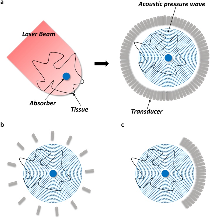
In the PAT, the acoustic pressure waves are generated by tissues excited with electromagnetic radiation pulsed laser or a continuous wave (CW) on a nanosecond timescale (Fig. 1a) [9]. The laser pulse duration is less than both thermal confinement and stress confinement threshold. In other words, the thermal diffusion and volume expansion of the absorber during laser pulse can be neglected. Considered the different light absorption coefficients of varying constituents in the tissue, the optical spectrum should be set to specific wavelengths, so it is capable of visualizing the anatomical features of the region of interest and simultaneously providing great penetration depths. Generally, the most commonly used optical wavelengths to excite the hemoglobin is ranged between 550 and 900 nm including the visible and near-infrared (NIR) spectrum [1]. After optical excitation, irradiated tissue converts the optical energy to heat and produces a slight temperature rise. The thermoelastic expansion of tissues leads to an initial pressure increase followed by a relaxation state, which produces acoustic waves that subsequently propagate throughout the space. Finally, these photoacoustic waves are recorded by either a single mechanically scanned detector or an array of transducers arranged in a specified geometry. The acoustic pressures detected by transducers are measured as time-resolved signals, which are used to reconstruct the initial pressure distributions, i.e., the image of the light-absorbing object, using reconstruction methods such as universal backprojection [10] and time-reversal [11,12].

Fig. 1.

Illustration of photoacoustic imaging. (a) Photoacoustic imaging process. (b) Sparse sensing. (c) Geometrical limitations (e.g., limited view).

Currently, reconstruction methods for PA images can be classified into two main categories: conventional reconstruction methods and learning-based reconstruction methods. Conventional reconstruction methods can be further distinguished into two sub-classes including direct reconstruction (e.g., universal backprojection [10] and filtered backprojection [13]) and model-based iterative reconstruction [14,15]. Direct reconstruction involves solving a single wave equation and therefore computation times for PAT reconstruction are dramatically faster. In comparison, model-based iterative reconstruction typically requires several iterations to minimize the difference between measured time-series signals and the predicted time-series signals evaluated by the PA forward model, which is computationally intensive.

More recently, PAT reconstruction based on machine learning has been developed. These also can be classified into two sub-classes: a direction reconstruction followed by learning-based post-processing reconstruction methods [16] and model-based learned iterative reconstruction methods [17,18]. The learning-based post-processing reconstruction method is applied after a single inversion step carried out by a conventional direct reconstruction. With this method, the artifacts and noise generated from the direct methods can be removed [19]. However, the performance of the learning-based post-processing reconstruction methods for PAT reconstruction is heavily dependent on the quality of the information content residing in the initial reconstruction [20]. In comparison, model-based learned iterative reconstruction combines the model-based approach with deep learning. A prior knowledge included in the model-based iterative reconstruction has been demonstrated its superior capability to reduce the artifacts and noise in the PAT reconstruction [21]. Learning-based iterative methods exploited this concept in the training phase; therefore, regularization term and weight originally handcrafted in the conventional model-based iterative methods are learned by the deep learning model [17]. This method includes the repeated simulation of the physical model into the network and leads to expensive computational costs as compared to learning-based post-processing methods. To dramatically reduce the computation times, this issue can be tackled by replacing the forward operator with faster approximate models without compromising reconstruction quality [22]. However, this method only addresses the high demanding computational cost. The limitation of the memory footprint remains an intractable issue.

To achieve a high-resolution of the initial pressure distribution of PAT, high spatial and temporal sampling rates are required simultaneously [23]. In the real-world application, temporal sampling rate above Nyquist rate can be satisfied by current transducers; however, the spatial sampling rate is limited by the experimental setup as a result of sparse sensing or geometrical limitations (e.g., limited view) (Fig. 1b and 1c) [24,25]. The sparse sensing strategy is typically used to enhance data acquisition speeds. Circumstance leading to the geometric limitations is due to the spatial structure of the imaging targets. For instance, breast imaging through PAT only allows in some specific geometric configurations such as planar-view system [26] and hemispherical array-based system [27,28]. Although high-resolution PA images can be obtained under the full-sampling configuration through the direct reconstruction methods, these methods are not optimal to account for the statistical characteristics of the measured data under the sparse sensing and geometric limitations scenario and, therefore, easily lead to artifacts in the PAT reconstruction. To overcome these issues, there is a need to develop advanced inversion algorithms.

In this study, the various types of learning-based methods recently proposed for PAT reconstruction in the sparse sensing scenario are tested and evaluated, including FD-UNet, Y-Net, U-Net, Pixel-DL, and the model-based learning. In addition, we propose some modified deep learning architectures (e.g., FD-YNet, PixelGAN, and PixelcGAN) that combine previously published models (e.g., Y-Net, GAN, and cGAN), which will also be evaluated. Characteristics of each method will be elucidated in the following sections. Due to the extensive computation times and memory constraints of the deep neural network for 3D imaged targets, this study is limited to 2D-PAT reconstruction for examining various learning-based methods. All methods are tested on the same imaging configuration setup for a fair comparison.

2. Background

PAT image reconstruction aims to recover an image from the endogenous tissues of interest. That is, the unknown optical-absorption coefficient $f^{*}\in X$ (which determines the initial pressure distribution) is reconstructed from measured acoustic pressure time series $g\in Y$ by solving the inverse problem where

$$g=A\left(f^{*}\right)+\delta g$$

Here, $A:X\to Y$ is denoted as a forward operator, modeling the measured acoustic pressure times series $g$ with a known defined linear operation. $\delta g\in Y$ is denoted as the additional measurement error (e.g., noise).

2.1. Signal generation in PAT

Initial acoustic pressure wave propagates throughout the space and is measured by a mechanically scanned ultrasonic transducer or transducer array. Mathematically, it can be defined as

$$p_0\left(\overrightarrow{r}\right)=\frac{\beta A_e}{\rho C_v\kappa }=\Gamma {\mu }_a(\overrightarrow{r})F\left(\overrightarrow{r};{\mu }_a,{\mu }_s,g\right)$$

Here $p_0$ is the initial acoustic pressure distribution. $\rho$ is the mass density. $C_v$ is the specific heat capacity at constant volume. $A_e$ is the absorption density, which is a product of the optical absorption coefficient ${\mu }_a$ and local optical fluence $F\left(\overrightarrow{r};{\mu }_a,{\mu }_s,g\right)$ where ${\mu }_s$ is scattering coefficients and $g$ is the anisotropy factor. $\kappa$ is the isothermal compressibility. $\beta$ is the thermal coefficient of volume expansion. $\Gamma =\frac{\beta }{\rho C_v\kappa }$, known as the Grueneisen parameter, is a dimensionless thermodynamic constant, determining the conversion efficiency of heat energy to pressure. This equation depicts that initial acoustic pressure distribution $p_0$ depends on the thermodynamic and optical parameters. Generally speaking, the thermodynamic parameter is assumed to be a spatially homogenous invariant in the variety of tissues and, therefore, the image contrast of $p_0$ is highly dominated by the product of the optical absorption coefficient ${\mu }_a$ and local optical fluence $F\left(\overrightarrow{r};{\mu }_a,{\mu }_s,g\right)$.

The PAT imaging starts at irradiating the target of interest with a short laser pulse, and thermal diffusion can be neglected if the laser pulse duration is much smaller than the thermal confinement threshold. Then, the acoustic pressure wave $p\left(r,t\right)$ at position $r$ and time $t$ satisfies the following equation

$$\left({\nabla }^2-\frac{1}{v_s^2}\frac{{\partial }^2}{\partial t^2}\right)p\left(r,t\right)=-\frac{p_0\left(r\right)}{v_s^2}\frac{d\delta \left(t\right)}{dt}$$

$\delta \left(t\right)$ represents a delta function. $v_s$ is the speed of sound. $p_0$ is the initial acoustic pressure distribution. In this study, forward wave propagation of irradiated tissues is computed by the k-space pseudospectral time-domain method equipped in the k-Wave Toolbox [29,30].

2.2. Model-based reconstruction

Model-based reconstruction aims to reconstruct the PA images by solving the optimization problem via an iteratively adjusting manner to improve the estimate where

$$\hat{f}≔\text{arg}\underset{f}{\text{min}}\left\{\frac{1}{2}{‖A\left(f\right)-g‖}_2^2+\lambda R\left(f\right)\right\}$$

Here $\frac{1}{2}{‖A\left(f\right)-g‖}_2^2$ is the fidelity term, measuring the distance between the measured acoustic pressure time series $g$ and predicted acoustic pressure time series estimated by the PA forward operator $A$. $R\left(f\right)$, termed as regularization functional, represents the prior knowledge regarding the structure encoded in the true solution of PA images. A weighting parameter $\lambda$ determines the amount of influence carried out by regularization functional against the need to data fit. While introducing the regularization functional can penalize the unfeasible solutions and avoid over-fitting, choosing unsuitable handcrafted parameters will result in poor reconstruction quality and even the need for a large number of iterations for a model to converge. Unlike the direct reconstruction methods in which reconstruction quality is susceptible to the imaging configuration setup, this method has been demonstrated to have superior reconstruction quality in terms of its generalizability and robustness [25].

2.3. Learning-based post-processing reconstruction

Deep learning involved in the post-processing reconstruction strategy requires the use of direct reconstruction methods (e.g., backprojection) as a pre-processing step for the initial reconstruction. Mathematically, let $A^{*}:Y\to X$ denotes as any direct reconstruction operator and $g^{\text{'}}\in Y$ represents measured acoustic pressure time series. The initial PA reconstruction $\stackrel{\sim }{f}\in X$ via direct reconstruction can be obtained as

$$\stackrel{\sim }{f}≔A^{*}\left(g^{\text{'}}\right)$$

Then, a deep neural network as a post-processing method is introduced to learn the removal of artifacts arisen from the direct reconstruction methods. These artifacts are severe due to imaging configurations where the direct reconstruction method is not applicable (e.g., geometric limitations and sparse sensing). This data-driven method in PA image reconstruction will be implemented in a supervised manner. Let ${\Lambda }_{\theta }$ to be the parameters of a deep neural network, the mathematical expression can be given as

$$\hat{f}≔{\Lambda }_{\theta }\left(\stackrel{\sim }{f}\right)$$

Under geometric limitations and sparse sensing scenarios, the direct reconstruction method easily leads to the loss of information and suffers with severe artifacts [20]. Therefore, the deep neural network must effectively use the remaining information as much as possible to learn the feature representations that are helpful for reconstruction. To learn the feature representations more effectively, several solutions based on deep neural networks specifically designed to eliminate artifacts in PA images were proposed [31,32]. Notably, these methods are established upon the well-known architecture, U-Net, which is a denoise algorithm widely used in the field of medical image reconstruction and segmentation.

2.4. Model-based learned iterative reconstruction

Rather than handcrafting fixed regularization functional as in conventional model-based iterative reconstruction, the penalty function is learned from the data in the training phase. Therefore, neural networks not only consider the information of PA reconstruction from each iteration, but the gradient information is also served as the required input for the model. This learning strategy is termed as deep gradient descent (DGD) or learned gradient scheme (LGS) originally proposed by [17] and defined as

$$f_{i+1}={\Lambda }_{{\theta }_i}\left(f_i,A^{*}\left(A\left(f_i\right)-g\right)\right)wherei=0,\cdots ,N-1$$

Here ${\Lambda }_{{\theta }_i}$ denotes as the learned updating parameters at $i$ th iteration. The predicted acoustic pressure time series is evaluated by the forward operator $A$. The gradient information is evaluated by the adjoint operator $A^{*}$. $g$ is the measured acoustic pressure times series. The PA reconstructed image $f_0$ for the first iteration is initialized by $A^{*}\left(A{f}_{true}+\delta g\right)$. Then, the objective function is defined as

$$L_{\theta }≔{‖f_N-f_{true}‖}_X^2$$

$f_N$ represents the reconstructed PA image of the last iteration and is the output of the ${\Lambda }_{{\theta }_{N-1}}$. $f_{true}$ denotes ground truth image. Typically, the gradient of the objective function $L_{\theta }$ is computed by performing the back-propagation from the last iteration to the first iteration. However, this end-to-end supervised training strategy is not suitable for model-based learned iterative reconstruction as a result of limited memory footprint and the expensive computation cost owing to the repetitive evaluation of forward and its adjoint operator. The most straightforward approach to address this issue is applying a “greedy” strategy while training the deep neural network, unrolling the entire model to multiple iterations, which each of the unrolled iteration updates parameters based on the objective function of its iteration [33]. Therefore, the objective function of each unrolled iteration in model-based learned iterative reconstruction will be adjusted to the following

$$L_{\theta i}={\left|\right|{\Lambda }_{{\theta }_i}\left(f_i,A^{*}\left(A\left(f_i\right)-g\right)\right)-f_{true}\left|\right|}_X^{2}wherei=0,\cdots ,N-1$$

The initialization of $f_0$ is the same as the original end-to-end training strategy; however, rather than updating parameters of the entire model, each unrolled iteration updates the parameters through its objective function instead.

3. Materials and methods

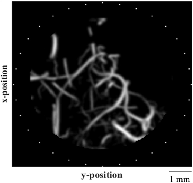
All synthetic data was generated by k-Wave, which is an open-source toolbox for MATLAB [34]. This versatile toolbox allows users to define arbitrary parameters such as the computational grid, photoacoustic sources, properties of the medium, and sensor configuration. In this study, the photoacoustic sources were defined inside the computational grid of 160 × 160, and the distance of each grid was defined as 50 micrometers shown in Fig. 8. The medium was assumed as non-absorptive and homogeneous with the speed of sound of 1500 m/s. The configuration with 32 sensors at equal space on a circle of radius of 4 mm was evaluated and tested. This sensor configuration can be regarded as a sparse sensing scenario, which involves the use of a small number of sensors for PA imaging. In this circumstance, high spatial resolution PA images typically cannot be obtained by direct reconstruction methods and easily result in artifact-robust images. Furthermore, a homogeneous internal fluence rate was assumed across all datasets. The number of samples and the time-step for the simulations were 768 samples and 10 ns, respectively. Here, we aimed to investigate the reconstruction performance in various types of learning-based reconstruction methods under the sparse sensing imaging strategy. Both learning-based post-processing and model-based learned iterative methods require the initial reconstruction of PA images by running the forward operator and reconstruction operator (e.g., time-reversal) to reconstruct initial PA images containing artifacts from the sparsely sampled data.

Fig. 8.

Sensor configuration with the imaged object. White dots represent sensors. Thirty-two sensors are evenly spaced on a circle with the radius of 4 mm.

3.1. Synthetic data for training and testing

Synthetic vasculature datasets were generated from a simple vasculature phantom. Augmentation techniques were used to increase the amount of data and diversified the complexity and trajectory of the vascular system. The detailed procedure of generating vasculature datasets is illustrated as follows. First, a simple vasculature phantom from the k-Wave toolbox was downsampled to the size of 128 × 128 so it can be fitted inside the defined computational grid. Next, the downsampled version of simple vasculature phantom increases its complexity by affine transformation; randomly choosing a scaling factor (0.75 to 1.25), rotation angle (0-359 degrees), translation factor (-10 to 10 pixels in the vertical and horizontal axis), and shearing factor along the horizontal axis. To maximize the diversity of the training dataset as much as possible, a generated vasculature phantom can further increase its complexity by superposition of a different number of transformed vasculature phantoms. Consequently, these richer features can be learned by deep neural networks, thereby improving the robustness and generalizability of models on the testing dataset. Here, we generated 500 vasculature phantoms as our ground truth for the training and the other 500 vasculature phantoms for the testing. These datasets will be simulated in the k-Wave using the above-defined configuration. Then, the measured acoustic pressure time-series signals are added with the gaussian noise and result in 24 dB signals. Lastly, artifact-robust PA reconstruction images were collected as the inputs for the models.

Besides, in vivo mouse cerebrovascular atlas was used to validate the reconstruction performance of various models in terms of their generalizability. This atlas, acquired by contrast-enhanced micro-CT, provided high-resolution volumetric images of vascular features [35]. The following pre-processing steps were performed to prepare the mouse neurovasculature data for validation tests: First, the Frangi vesselness filter was applied to extract the vessel-like features in the volume [36], and the thresholding technique was used to remove the remaining background. Next, two hundred sub-volumes with the size of 128 × 128 × 128 are randomly sampled and followed by maximum intensity projections (MIPs). To maintain realistic in vivo features, data augmentation was not performed on MIPs. The procedure of simulating the photoacoustic data acquisition was the same as those described above for synthetic vasculature images.

3.2. FD-UNet architecture

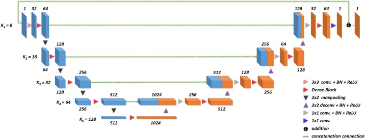
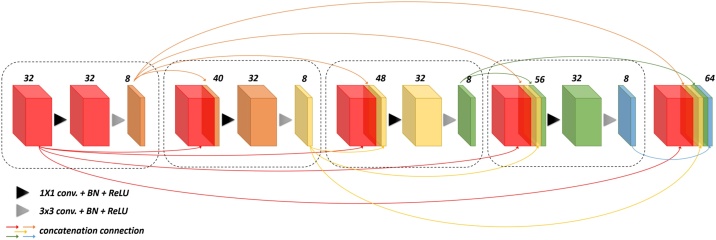
FD-UNet as shown in Fig. 2 was proposed by [19], developed mainly for the removal of artifacts in the PA images. This architecture was modified upon the well-known segmented and denoised U-Net architecture [37]. Unlike the U-Net which includes a sequence of two convolution operations in each spatial level, FD-UNet exploits the dense block concept proposed in the dense convolutional network (DenseNet) instead [38]. In a dense block shown in Fig. 3, previous convolutional layers are concatenated channel-wise to all subsequent convolutional layers. Namely, the features extracted from the previous convolution operations are reused for later convolution operations. This strategy makes deep neural networks have the so-called memory and reduce the need for learning redundant features. k values, user-defined parameters, in Fig. 2 denote the growth rate for the dense block in each spatial level.

Fig. 2.

Illustration of FD-UNet architecture. The number of feature maps in each spatial level is indicated above or below the corresponding cube. Hyperparameter, k, denotes the growth rate of the dense block in each spatial level. Feature maps learned in the encoder are concatenated to the same spatial level in the decoder.

Fig. 3.

Illustration of four layers of a dense block. Here, the growth rate, k, is set to 8, and the initial number of feature maps is 32. Each black-dashed box represents one layer in the dense block. After going through the operation of four layers of a dense block, 64 feature maps are generated.

To avoid the vanishing gradient problem and make networks learn more efficiently, an identity mapping strategy is introduced. Mathematically, FD-UNet can be expressed as

$$y={\Lambda }_{\theta }\left(x\right)+x$$

Here $x$ is the input, and $y$ is the reconstructed output of the deep neural network. ${\Lambda }_{\theta }$ denotes the network parameters. FD-UNet aims to remove the artifacts in PA images by learning the residual function $A_{\theta }\left(x\right)$ with a shortcut connection. This element-by-element addition neither introduces additional parameters for the model nor does it increase computational cost [39].

3.3. Y-Net and FD-YNet architecture

Most proposed CNN architectures for denoising and artifacts removal of PA imaging are based either using the measured signals or textural images as the only input [40]. In the case of measured signals as the only input, learning-based models do not rely on the knowledge of the physical model for reconstruction. Conversely, learning-based models based on the direct reconstruction methods are typically compromised by severe artifacts, particularly, when the number of sensors is not enough to sample the whole information in the imaged target. To solve the drawbacks of these two methods respectively, [41] developed the hybrid processing network, termed as Y-Net, devoted to reducing artifacts in the PA images and is built upon the U-Net as well.

Unlike the U-Net which has one contracting path, Y-Net has two contracting paths instead. It requires inputs of a training pair, comprising of the measured acoustic pressure time-series signals and its corresponding rough PA solution reconstructed by direct methods (e.g., backprojection and time-reversal). Features extracted by both contracting paths will later be concatenated and served as the inputs for a symmetric expanding path. Mathematically, the parameter update of the Y-Net can be solved by

$$\text{arg}\text{min}{\mathbb{E}}_{\left(\stackrel{\sim }{f},g^{\text{'}}\right),f}=\left|\right|{\Lambda }_{\theta }\left(\stackrel{\sim }{f},g^{\text{'}}\right)-f{\left|\right|}_X^2$$

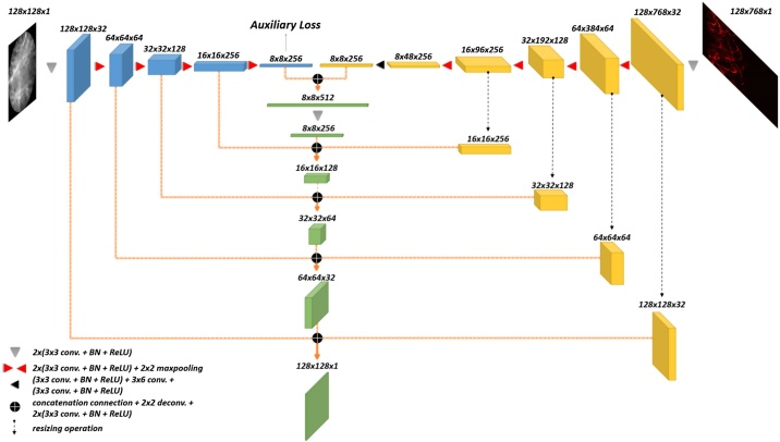
Here, $f\in X$ is the ground truth images. $\stackrel{\sim }{f}\in X$ is the initial PA reconstruction via a direct reconstruction method. $g^{\text{'}}\in Y$ represents measured acoustic pressure time-series signals. ${\Lambda }_{\theta }$ denotes the model parameters. The auxiliary loss is also included to penalize the encoder which is responsible for learning the features of textural information. This can be written as

$$L_{aux}\left(z\right)=\frac{1}{2}{‖z\left(\stackrel{\sim }{f}\right)-R\left(f\right)‖}_X^2$$

Here, $z$ represents the encoder for learning the features from the textural images. $R$ is a resizing operation. Consequently, Y-Net is trained by minimizing the total loss described as

$$L_{total}=L_{rec}+{\lambda L}_{aux}$$

$\lambda$ is a hyper-parameter, determining the weight of the auxiliary loss. $L_{rec}$ denotes the reconstruction loss.

To implement Y-Net according to our sensor configuration settings, the original framework is needed to be modified and its entire network is shown in Fig. 4. In addition to the difference in spatial dimensions of the encoder for measured time-series signals, all the above-mentioned conceptual elements remain the same in the modified framework. In our implementation, the dimension of measured pressure acoustic time-series signals is 32 × 768 pixels where each row represents a sensor channel, and each column corresponds to the signal measured in that specific timestep. The number of sensors is 32 in our configuration settings; therefore, there are 32 rows in the measured data. On the other hand, the input to the other contracting path is an approximate reconstruction image that has dimensions 128 × 128. The dimension mismatch in the inputs of the two contracting paths is addressed by zero-padding the time-series data in the row dimension to achieve a time-series input that is 128 × 768 in dimension. Besides, an extra 3 × 6 convolution operation is inserted in the middle of the lowest spatial level, transforming the spatial size of 8 × 48 feature maps to 8 × 8 feature maps. Similar to the U-Net, feature maps of each spatial level in the encoder are concatenated to the decoder of the same spatial level. Furthermore, because of the asymmetry in the dimension of measured data, a resizing operation is performed before the concatenated connection. For the $\lambda$, we choose 0.5 to be the same as the originally proposed research.

Fig. 4.

Illustration of Y-Net architecture. Resizing operations are performed in the contracting path which is responsible for learning the feature representation in measured data. Then, the feature maps in each spatial level of the two contracting paths are concatenated to their respective spatial levels in the decoder. Furthermore, an auxiliary loss is included at the bottom of the contracting path responsible for learning the texture information. The spatial dimension of feature maps is indicated above the corresponding cube.

In addition to evaluating the original Y-Net architecture, the modified network, termed as FD-YNet, is proposed. This proposed network is built upon the Y-Net and incorporates the dense blocks used in the FD-UNet. Namely, in each spatial level, a sequence of two convolution operations is replaced with a dense block.

3.4. Pixel-DL architecture

Initial inversion through the direct reconstruction methods suffers from severe artifacts and loss of information when mapping the measured time-series signals to image space. Similar to Y-Net, authors who developed the Pixel-DL shown in Fig. 5 aims at making more effective use of measured time-series signals in the PA image reconstruction [42].

Fig. 5.

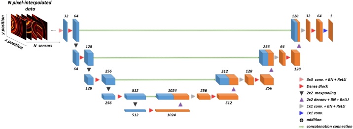
Illustration of Pixel-DL. Unlike the FD-UNet, which requires a direct reconstruction method as the initial inversion for the input, Pixel-DL replaces the poor solution of the PA images with pixel-wise interpolated channel maps. N denotes the number of sensors or the number of pixel-wise interpolated channels.

Unlike the Y-Net, which directly introduces the measured time-series signals into the model, the initial inversion originally performed by the direct reconstruction methods is replaced with a technique termed pixel-wise interpolation. To use this technique, assumptions must be made for acoustic wave propagation: (1) defined computational grid is an acoustic homogeneous medium (2) the acoustic waves propagate spherically at a constant speed of sound. If the medium is heterogeneous, the modified pixel-wise interpolation is necessary. Under these assumptions, the acoustic pressure time-series signals recorded by a specific sensor will be mapped to each pixel position in the defined computational grid. Consequently, the total number of mappings corresponds to the number of sensors. Notably, pixel-wise interpolation does not introduce the artifacts as such in direct reconstruction methods; hence, the deep neural network does not need to learn the extra task for removing artifacts. The only task for the model is to learn to map the pixel-interpolated data to the original image space. Besides, the architecture of the Pixel-DL is essentially an FD-UNet. However, the only difference is that the identity mapping is removed due to the asymmetric dimension of the input-output pair.

3.5. PixelGAN and PixelcGAN architecture

Recently, an increasing number of medical imaging fields have used generative adversarial networks (GANs) for solutions, especially in the fields of reconstruction [32], medical image synthesis [43], segmentation [44], classification [45], and detection [46]. While GANs are applied in a wide variety of fields, each field has its domain-specific framework applicable to a specific task. For instance, in the field of medical image reconstruction, the fundamental of image-to-image translation is dominated in all medical tomography modalities [47]. Therefore, we build networks based on this concept.

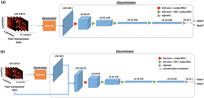
GANs aim to approximate the data distribution of generated output to the real data without the need to explicitly model the underlying probability density function [48]. It comprises two networks including a generative model and a discriminative model. In our implementation, the generative model, essentially a Pixel-DL, takes the pixel-interpolated data $x$ as the input, and the corresponding distribution of input data denotes as $p\left(x\right)$. The ouput of generative model $G(x)$ is expected to approximate the real data $y$ that is sampled from the real data distribution $p\left(y\right)$. The goal of the generative model is to approximate the generated data distribution as close as possible to the real data distribution. For the discriminative model, PatchGAN developed by [49] is introduced. This network takes the generated data or real data as the input and outputs a N x N patch in an image, indicating the probability that the input to the discriminative model is the generated data or real data. Here, we term this modified network as PixelGAN, and its entire network is illustrated in Fig. 6a. The objective of PixelGAN can be expressed as

$$L_{PixelGAN}\left(G,D\right)={\mathbb{E}}_{p(y)}\left[logD\left(y\right)\right]+{\mathbb{E}}_{p(x)}[\text{l}\text{o}\text{g}(1-D(G(x))]$$

Fig. 6.

Illustration of PixelGAN and PixelcGAN. (a) PixelGAN: pixel-interpolated data is served as the input of the generator (Pixel-DL), and the discriminator (PatchGAN) classifies input as real or fake. (b) PixelcGAN: pixel-interpolated data is simultaneously served as the input of generator and discriminator, and discriminator classifies the output based on the concatenation of condition and generated output.

In the training phase, the $L1$ distance is included in the generative model. Therefore, the generative model not only learns to fool the discriminative model but manages to approximate the real data as close as possible. Consequently, the total loss of PixelGAN can be written as

$$L_{total}=\text{arg}\underset{G}{\text{m}\text{i}\text{n}}\underset{D}{\text{m}\text{a}\text{x}}{L}_{PixelGAN}\left(G,D\right)+\lambda L(G)$$

For the $\lambda$, we choose 100 as suggested in [49]. Besides, conditional GAN is tested and evaluated. The architecture of the network and parameter $\lambda$ remain the same as the PixelGAN. The only difference is that the pixel-interpolated data not only serves as the input of the generative model but as the condition for the discriminative model. Here, we term this modified conditional GAN as PixelcGAN, and its entire network is illustrated in Fig. 6b. The objective of PixelcGAN can be given as

$$L_{PixelcGAN}\left(G,D\right)={\mathbb{E}}_{p\left(x\right),p(y)}\left[logD\left(x,y\right)\right]+{\mathbb{E}}_{p\left(x\right)}[\text{l}\text{o}\text{g}(1-D(x,G(x))]$$

Similar to PixelGAN, $L1$ distance also includes when training the generative model. Ultimately, the total loss of PixelcGAN can be defined as

$$L_{total}=\text{a}\text{r}\text{g}\underset{G}{\text{min}}\underset{D}{\text{max}}{L}_{PixelcGAN}\left(G,D\right)+\lambda L(G)$$

3.6. Model-based learned iterative reconstruction

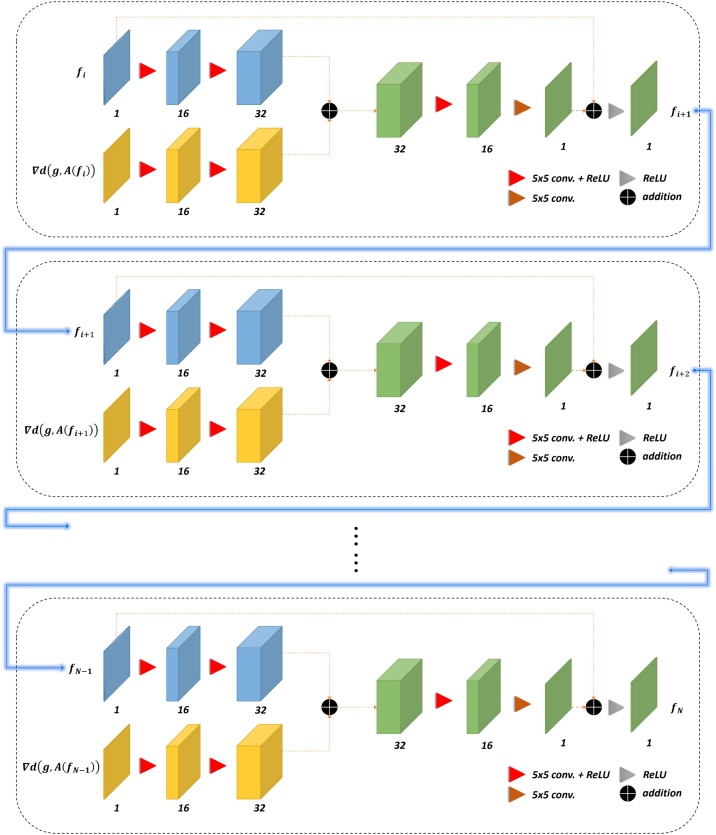
Model-based learned iterative reconstruction shown in Fig. 7 was proposed by [17]. This method is characterized as the repetitive use of physical models and deep neural networks to enhance the reconstruction performance. In the original study, this method was implemented for 3D imaged targets. Therefore, there is a need for calibrating some parameters in accordance with our configuration settings, such as replacing the 3D convolutional operation with the 2D convolutional operation. Besides, forward operation and reconstruction operation is performed through a 2D forward operator and its adjoint operator. Except for the above modifications, the model architecture and hyper-parameters are exactly the same. The technical details regarding model-based learned iterative reconstruction are elaborated in the background section.

Fig. 7.

Illustration of model-based learned iterative reconstruction method. Except for the first iteration, each following iteration (black-dashed box) requires the output of the previous iteration as the input; furthermore, gradient information is computed by running the forward and its adjoint operator. N-1 determines the number of iterations. The number of feature maps is presented at the bottom of the corresponding cube.

To initialize the first iteration of the model-based learned iterative reconstruction, initial reconstruction and gradient information are required. First, forward operator was used to simulate measured time-series signals. Next, the simulated measured time-series signals were added with the gaussian noise resulting in 24-dB peak signal-to-noise ratio. Subsequently, noised data was applied with the adjoint operator to obtain the initial reconstructed photoacoustic images. To prepare the gradient information, the initial reconstructed photoacoustic images were applied with the forward operator and newly measure time-series signals were simulated. The gradient information was produced by running the adjoint operator on the difference between the initial measured time-series signals and newly measure time-series signals. After the training for the first iteration, the second iteration can be initialized by the predicted outputs from the first iteration, serving as one of the required inputs for the second model. In addition, the gradient information for the second iteration was prepared by running the adjoint operator on the difference between the initial measured time-series signals and the predicted measure time-series signals. This process remains the same for the subsequent iterations. In our implementation, the final reconstructed photoacoustic images were obtained at the fifth iteration.

3.7. Deep learning implementation

The experimental platform is based on Windows 10 64-bit operating system, Intel i7-10750H CPU, 16 G memory, and a single RTX 2070 SUPER GPU (8 GB). All proposed and modified deep neural networks are then implemented in Python 3.6 with an open-source deep-learning library (e.g., Tensorflow v2.0). Here, Adam, an algorithm for first-order gradient-based optimization, with a learning rate of 1e^-4 is selected. The mini-batch size is set as four images, and all models are trained with 1,000 epochs. The training loss shown in Fig. A9 indicates that all the models converge with minimal changes in training loss by 1,000 epochs.

4. Experiments and results

To determine the PA image reconstruction performance of the models, evaluation methods such as qualitative and quantitative measurements are used. For qualitative measurement, not only the reconstruction results are visualized, error distributions between the reference and results of models’ reconstruction are also displayed. For the quantitative measurement, structural similarity index (SSIM) [50] and its decomposed components (e.g., luminance, contrast, and structure) and peak signal-to-noise ratio (PSNR) are used as metrics to measure the quality of PA image reconstruction. To have a fair comparison, the complexity of the models is matched as much as possible without modifying the architecture of the originally proposed models. Besides, we also investigate the impact of different forms of input on the models’ reconstruction performance.

4.1. Validation on synthetic and in vivo mouse cerebral vasculature dataset

In this experiment, the synthetic vasculature and in vivo mouse cerebral vasculature are simulated by 32 equidistant sensors on a circle of radius of 4000 micrometers. While different forms of input are required according to the characteristics of the model, all models are trained with the dataset simulated from the same synthetic vasculature dataset. Training and testing on the synthetic vasculature provide us with the reconstruction performance of the models in a scenario when the image domain is well-matched. On the other hand, training with synthetic vasculature but testing on in vivo mouse cerebral vasculature evaluate the reconstruction performance of the models in a scenario when the image domain is mismatched, and more importantly, determining the generalizability of the models.

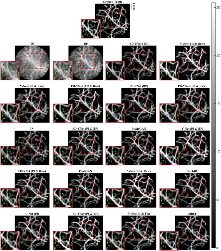
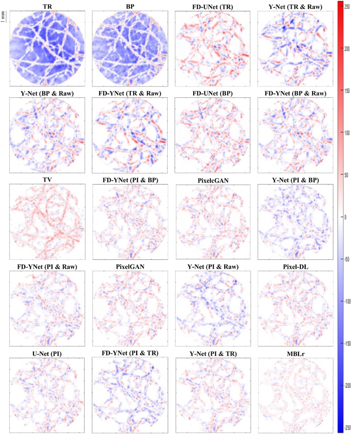
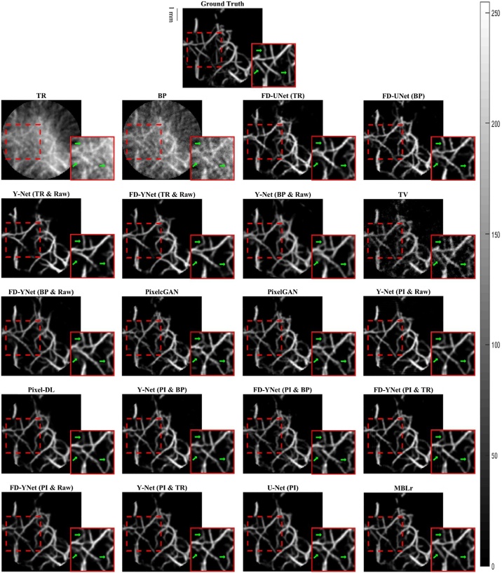
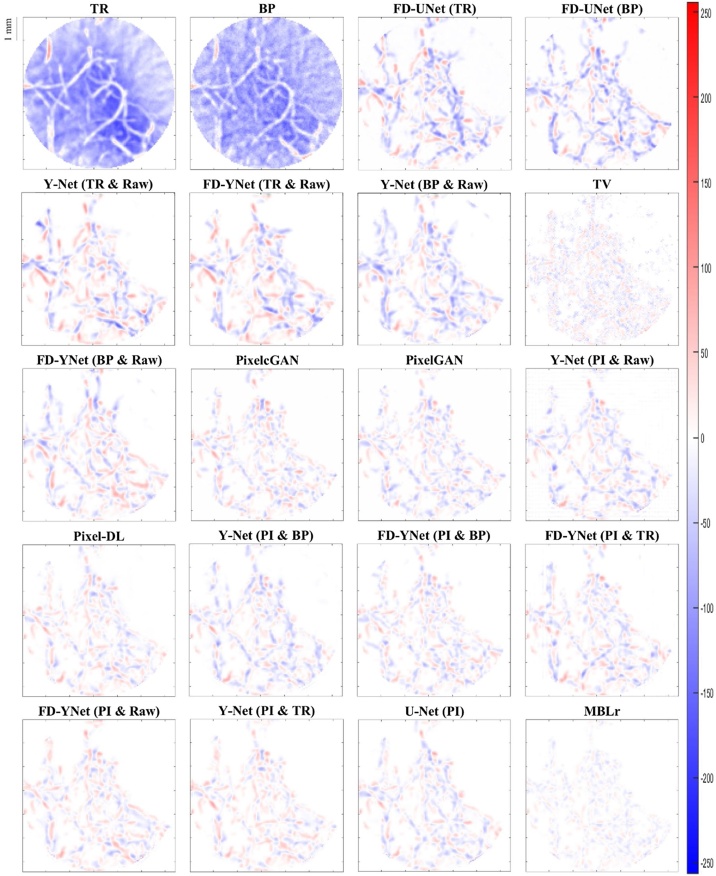
The visual comparison of reconstruction performance for synthetic vasculature in different models is shown in Fig. 9. Here, only the results reconstructed from the models with around 30 million parameters are shown: the appendix provides the results reconstructed from the other complexities of the model. Besides, error maps are displayed in Fig. 10. Positive values (red) shown in error maps represent that pixel intensity is less than reference. Conversely, negative values (blue) indicate that pixel intensity is greater than a reference and should not be located at that specific pixel location. We also investigate the impact of different forms of inputs on the PA image reconstruction. Four different inputs are evaluated: measured raw PA signals, time reversal, backprojection, and pixel-interpolated data. Notably, the backprojection images are generated from the pixel-interpolated data by summing along the channel axis. Compared to time-reversal reconstruction which requires solving the inverse wave equation, backprojection operation greatly reduces the computation times. Furthermore, the quantitative results tested on the synthetic vasculature are shown in Table 1 and Table 2. To evaluate the generalizability of the models, visual comparisons of the reconstruction performance for the mouse cerebral vasculature are shown in Fig. 11, and error maps are displayed in Fig. 12. Additionally, the quantitative results of the mouse cerebral vasculature are shown in Table 3 and Table 4.

Fig. 9.

Visualization of PA image reconstruction for synthetic vasculature in different models. The reconstruction results are ordered from the worst to the best (left to right and top to bottom) according to the SSIM metric. The abbreviations in parentheses represent the form of the data as the inputs to the models. TR: time-reversal image. BP: backprojection image. TV: total variation. Raw: measured time-series signals. PI: pixel-interpolated data. MBLr: model-based learning.

Fig. 10.

Error maps of PA image reconstruction for synthetic vasculature in different models. The reconstruction results are ordered from the worst to the best (left to right and top to bottom) according to the SSIM metric. Positive values (red) represent that pixel intensity is less than reference. Negative values (blue) represent that pixel intensity is larger than the reference. The abbreviations in parentheses represent the form of the data as the inputs to the models. TR: time-reversal image. BP: backprojection image. TV: total variation. Raw: measured time-series signals. PI: pixel-interpolated data. MBLr: model-based learning.

Table 1.

Comparison of reconstruction performance for synthetic vasculature in different models trained with either textural images or both the textural images and measured time-series signals.

Dataset	Synthetic Vasculature
Network	Parameters	PSNR	SSIM	SSIM Luminance	SSIM Contrast	SSIM Structure	Exec.
FD-UNet (TR)	37,888,449	20.802 ± 1.835	0.584 ± 0.053	0.741 ± 0.074	0.907 ± 0.021	0.832 ± 0.047	42 ms
FD-UNet (BP)		21.923 ± 1.959	0.637 ± 0.052	0.779 ± 0.069	0.928 ± 0.017	0.852 ± 0.043
Y-Net (TR & Raw)	37,506,354	20.778 ± 2.233	0.713 ± 0.064	0.850 ± 0.034	0.913 ± 0.017	0.851 ± 0.049	48 ms
Y-Net (BP & Raw)		21.856 ± 2.159	0.736 ± 0.065	0.868 ± 0.031	0.920 ± 0.020	0.863 ± 0.045
FD-YNet (TR & Raw)	34,852,306	21.064 ± 2.150	0.722 ± 0.060	0.853 ± 0.031	0.910 ± 0.019	0.855 ± 0.047	70 ms
FD-YNet (BP & Raw)		22.204 ± 2.209	0.739 ± 0.061	0.868 ± 0.034	0.927 ± 0.018	0.865 ± 0.043

The abbreviations in parentheses represent the data form used by the models. TR: time-reversal image. BP: backprojection image. Raw: measured time-series signals. PI: pixel-interpolated data.

Table 2.

Comparison of reconstruction performance for synthetic vasculature in different models trained with either the pixel-interpolated data or the combination of pixel-interpolated data with another form of input.

Dataset	Synthetic Vasculature
Network	Parameters	PSNR	SSIM	SSIM Luminance	SSIM Contrast	SSIM Structure	Exec.
Y-Net (PI & Raw)	37,524,210	23.747 ± 2.320	0.817 ± 0.037	0.912 ± 0.015	0.957 ± 0.009	0.909 ± 0.029	49 ms
FD-YNet (PI & Raw)	34,861,234	24.400 ± 2.167	0.828 ± 0.044	0.920 ± 0.019	0.954 ± 0.013	0.914 ± 0.029	76 ms
Y-Net (PI & TR)	32,809,717	25.090 ± 2.299	0.821 ± 0.030	0.906 ± 0.013	0.958 ± 0.012	0.924 ± 0.027	27 ms
FD-YNet (PI & TR)	27,790,517	23.800 ± 2.297	0.835 ± 0.043	0.924 ± 0.020	0.958 ± 0.011	0.912 ± 0.030	47 ms
Y-Net (PI & BP)	32,809,717	24.392 ± 2.481	0.826 ± 0.042	0.914 ± 0.018	0.963 ± 0.008	0.915 ± 0.030	27 ms
FD-YNet (PI & BP)	27,790,517	24.804 ± 2.295	0.812 ± 0.038	0.906 ± 0.019	0.959 ± 0.011	0.908 ± 0.030	47 ms
UNet (PI)	31,062,145	24.942 ± 2.234	0.831 ± 0.037	0.918 ± 0.014	0.955 ± 0.014	0.925 ± 0.026	24 ms
Pixel-DL (PI)	37,906,305	24.957 ± 2.204	0.815 ± 0.030	0.902 ± 0.011	0.958 ± 0.013	0.922 ± 0.027	42 ms
PixelGAN (PI)	G: 37,906,305 D: 1,711,041	24.538 ± 2.182	0.822 ± 0.040	0.917 ± 0.020	0.958 ± 0.011	0.907 ± 0.029	42 ms
PixelcGAN (PI)	G: 37,906,305 D: 1,743,809	24.571 ± 2.214	0.813 ± 0.044	0.907 ± 0.029	0.957 ± 0.011	0.907 ± 0.030	42 ms
Model-Based Learninga	198,565	29.590 ± 2.694	0.930 ± 0.026	0.971 ± 0.011	0.985 ± 0.006	0.966 ± 0.014	∼ 6 s
TV	-	23.774 ± 2.403	0.721 ± 0.037	0.869 ± 0.025	0.914 ± 0.023	0.863 ± 0.035	345 s

The abbreviations in parentheses represent the data form used by the models. TR: time-reversal image. BP: backprojection image. TV: total variation. Raw: measured time-series signals. PI: pixel-interpolated data. G: generator. D: discriminator. ^aTrained with the data evaluated by repeated forward and adjoint operators and reconstructed outputs from the previous iteration.

Fig. 11.

Visualization of PA image reconstruction for mouse cerebral vasculature in different models. The reconstruction results are ordered from the worst to the best (left to right and top to bottom) according to the SSIM metric. The abbreviations in parentheses represent the form of the data as the inputs to the models. TR: time-reversal image. BP: backprojection image. TV: total variation. Raw: measured time-series signals. PI: pixel-interpolated data. MBLr: model-based learning.

Fig. 12.

Error maps of PA image reconstruction for mouse cerebral vasculature in different models. The reconstruction results are ordered from the worst to the best (left to right and top to bottom) according to the SSIM metric. Positive values (red) represent that pixel intensity is less than reference. Negative values (blue) represent that pixel intensity is larger than the reference. The abbreviations in parentheses represent the form of the data as the inputs to the models. TR: time-reversal image. BP: backprojection image. TV: total variation. Raw: measured time-series signals. PI: pixel-interpolated data. MBLr: model-based learning.

Table 3.

Comparison of reconstruction performance for mouse cerebral vasculature in different models trained with either textural images or both the textural images and measured time-series signals.

Dataset	Mouse Cerebral Vasculature
Network	Parameters	PSNR	SSIM	SSIM Luminance	SSIM Contrast	SSIM Structure	Exec.
FD-UNet (TR)	37,888,449	19.779 ± 1.116	0.599 ± 0.028	0.838 ± 0.039	0.907 ± 0.016	0.744 ± 0.044	42 ms
FD-UNet (BP)		20.808 ± 1.189	0.643 ± 0.025	0.863 ± 0.036	0.926 ± 0.012	0.771 ± 0.040
Y-Net (TR & Raw)	37,506,354	19.000 ± 1.545	0.623 ± 0.048	0.836 ± 0.029	0.900 ± 0.016	0.766 ± 0.046	48 ms
Y-Net (BP & Raw)		20.973 ± 1.246	0.667 ± 0.043	0.857 ± 0.029	0.922 ± 0.014	0.796 ± 0.041
FD-YNet (TR & Raw)	34,852,306	19.580 ± 1.376	0.621 ± 0.052	0.818 ± 0.036	0.896 ± 0.020	0.776 ± 0.044	70 ms
FD-YNet (BP & Raw)		21.222 ± 1.346	0.674 ± 0.043	0.867 ± 0.025	0.925 ± 0.014	0.796 ± 0.041

The abbreviations in parentheses represent the data form used by the models. TR: time-reversal image. BP: backprojection image. Raw: measured time-series signals. PI: pixel-interpolated data.

Table 4.

Comparison of reconstruction performance for mouse cerebral vasculature in different models trained with either pixel-interpolated data or the combination of pixel-interpolated data with another form of input.

Dataset	Mouse Cerebral Vasculature
Network	Parameters	PSNR	SSIM	SSIM Luminance	SSIM Contrast	SSIM Structure	Exec.
Y-Net (PI & Raw)	37,524,210	21.953 ± 1.633	0.746 ± 0.031	0.904 ± 0.014	0.948 ± 0.007	0.841 ± 0.030	49 ms
FD-YNet (PI & Raw)	34,861,234	23.190 ± 1.301	0.753 ± 0.036	0.904 ± 0.019	0.947 ± 0.009	0.849 ± 0.031	76 ms
Y-Net (PI & TR)	32,809,717	23.809 ± 1.423	0.767 ± 0.025	0.908 ± 0.014	0.949 ± 0.009	0.863 ± 0.028	27 ms
FD-YNet (PI & TR)	27,790,517	21.983 ± 1.593	0.738 ± 0.039	0.891 ± 0.020	0.944 ± 0.009	0.844 ± 0.031	47 ms
Y-Net (PI & BP)	32,809,717	22.432 ± 1.641	0.754 ± 0.033	0.911 ± 0.012	0.953 ± 0.006	0.843 ± 0.031	27 ms
FD-YNet (PI & BP)	27,790,517	23.544 ± 1.376	0.752 ± 0.033	0.911 ± 0.015	0.954 ± 0.006	0.839 ± 0.030	47 ms
UNet (PI)	31,062,145	23.676 ± 1.379	0.770 ± 0.033	0.915 ± 0.014	0.948 ± 0.010	0.863 ± 0.028	24 ms
Pixel-DL (PI)	37,906,305	23.653 ± 1.351	0.767 ± 0.026	0.912 ± 0.011	0.948 ± 0.009	0.862 ± 0.028	42 ms
PixelGAN (PI)	G: 37,906,305	23.285 ± 1.339	0.747 ± 0.035	0.906 ± 0.016	0.951 ± 0.007	0.837 ± 0.029	42 ms
	D: 1,711,041
PixelcGAN (PI)	G: 37,906,305	23.303 ± 1.369	0.744 ± 0.033	0.902 ± 0.020	0.950 ± 0.007	0.838 ± 0.030	42 ms
	D: 1,743,809
Model-Based Learninga	198,565	27.960 ± 1.708	0.872 ± 0.026	0.953 ± 0.011	0.979 ± 0.005	0.925 ± 0.020	∼ 6 s
TV	-	23.327 ± 1.404	0.719 ± 0.031	0.915 ± 0.020	0.948 ± 0.016	0.802 ± 0.036	345 s

The abbreviations in parentheses represent the data form used by the models. TR: time-reversal image. BP: backprojection image. TV: total variation. Raw: measured time-series signals. PI: pixel-interpolated data. G: generator. D: discriminator. ^aTrained with the data evaluated by repeated forward and adjoint operators and reconstructed outputs from the previous iteration.

The error maps in Fig. 10 and Fig. 12 indicate that the direct reconstruction methods (e.g., time reversal and backprojection) suffer from severe artifacts in the background. Comparing these two reconstructed images, the time-reversal image has more severe artifacts than the backprojection image, which can be seen because of the darker blue background. Then, we compare the reconstruction performance of the FD-UNet and Y-Net on the synthetic vasculature and mouse cerebral vasculature. To conduct a fair comparison, the number of parameters is matched in two different neural networks, and the form of the input data (e.g., time-reversal or backprojection) is the same for both models. Besides, Y-Net requires measured PA time-series signals as an additional input. In terms of reconstruction performance, Y-Net provides greater reconstruction performance than the FD-UNet when the domain of training and testing sets are well-matched. In terms of generalizability, the reconstruction performance of the FD-UNet is more stable than the Y-Net when the domain of training and testing sets are not well-matched. The quantitative results of these two models performed on synthetic vasculature and mouse cerebral vasculature are shown in Table 1 and Table 3, respectively. Furthermore, we compare the Y-Net with the FD-YNet, which replaces the sequence of two convolution operations with a dense block in each spatial level. The quantitative results shown in Table 1 and Table 3 suggest that including the dense blocks in the originally proposed Y-Net does not significantly increase the reconstruction performance of the model.

Next, pixel-interpolated data is served as the input for Y-Net, FD-YNet, U-Net, Pixel-DL, pixelGAN, and pixelcGAN. Although Y-Net and FD-YNet allow another form of input data such as time-reversal and backprojection images to provide texture information, the reconstruction performance of the models apparently does not benefit from this additional information. Error maps in Fig. 10 and Fig. 12 and quantitative results in Table 2 and Table 4 demonstrate that there is no significant difference between models when they are all trained with the pixel-interpolated data. Interestingly, amongst all post-processing methods, U-Net with the fewest parameters has the best reconstruction performance when testing on the mouse cerebral vasculature, indicating that intricate model architecture and additional information (e.g., measured time-series signals and textural images) are not as necessary when pixel-interpolated data is used for training. In terms of generalizability, the reconstruction performance of the models trained with the pixel-interpolated data decreases when the domain of training and testing sets are not well-matched. However, compared to the models trained with either textural images or the combination of textural images and measured time-series signals, pixel-interpolated data as an only input for the models significantly improves the PA image reconstruction in both synthetic vasculature and mouse cerebral vasculature.

4.2. Model robustness on synthetic and in vivo mouse cerebral vasculature dataset

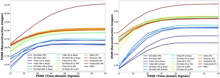
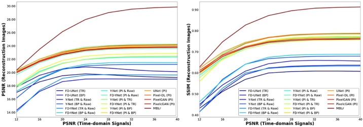
In this experiment, the robustness of the models is tested by different levels of noise (12 to 40 dB PSNR with the step size of 4) included in the synthetic and mouse cerebral vasculature datasets. All the models are trained with the 24 dB PSNR synthetic vasculature. Fig. 13 and Fig. 14 demonstrate that model-based learning has the best reconstruction performance at all different levels of noise. Besides, models trained with pixel-interpolated data have a greater performance at all levels of noise compared to the models trained with either the textural images or the combination of textural images and measured PA time-series signals. Furthermore, models trained with pixel-interpolated data have less variability in SSIM at different levels of noise, implying that different models have no significant difference in reconstruction performance.

Fig. 13.

Model performance under synthetic vasculature with different levels of noise. Left panel: PSNR is used as a metric for different levels of noise. Right panel: SSIM is used as a metric for different levels of noise.

Fig. 14.

Model performance under mouse cerebral vasculature with different levels of noise. Left panel: PSNR is used as a metric for different levels of noise. Right panel: SSIM is used as a metric for different levels of noise.

Interestingly, the robustness test shows that the learning-based post-processing models tested on the data where the noise is less than the training dataset stagnate or only slight increase in the reconstruction performance. Furthermore, none of these models exhibited significant improvement in image-reconstruction performance when the PSNR of the data gradually increases from 24 dB to 40 dB. In comparison, model-based learning results in a continuous, albeit slower, increase in image reconstruction as the PSNR of the time-domain signal incrementally increases from 24 dB to 40 dB. Consequently, the robustness test indicates that model-based learning is more adept at generalizing when reconstructing PA images from data acquired at different PSNRs.

5. Discussion and conclusion

In this study, we present a comprehensive study to compare the recently proposed learning-based PA image reconstruction methods in the scenario of sparse sensing. The results show that including the measured time-series signals as an additional input to the neural network indeed enhances the reconstruction performance of the models when the domain of training and testing sets are well-matched. Prior work indicated that models trained with the measured time-series signals prone to overfit on the training set [42]. Including textural information with the measured time-series signals greatly reduces the overfitting of the training set. However, the measured time-series signals as an additional input do not significantly improve the reconstruction performance of the models when the training and testing domains are mismatched. Moreover, our results show that introducing the dense blocks into the Y-Net does not significantly increase the reconstruction performance.

Interestingly, we demonstrate that models trained with pixel-interpolated data significantly outperform the models trained with either the textural images or the combination of textural images and measured time-series signals. In other words, the reconstruction performance of the models depends on the form of input data. Compared to the textural images (e.g., time-reversal and backprojection), pixel-interpolated data contains high-quality information and does not suffer from the artifacts. Compared to the measured time-series signals, pixel-interpolated data provides an efficient approach for the model to learn the projection from channel maps to image space since the convolutional operation can be fundamentally recognized as the projection operation. Furthermore, we suggest that the pixel-interpolated data can be applied to a simplified model (e.g., U-Net), implying that the richness of information it carries does not require an intricate model for reconstruction.

Among these PA image reconstruction methods, model-based learning outperforms all other learning-based post-processing methods. Limited by repeated simulations, the reconstruction time of the model-based learning takes longer than the learning-based post-processing methods. To address this problem, some solutions have recently been proposed to reduce the training and reconstruction time of model-based learning methods, for instance, replacing the forward operator with an approximate model [22] and exploiting multi-scale learned iterative reconstruction methods [51]. These methods greatly reduce the computation times without compromising the reconstruction performance of the models under the scenario of sparse sensing and limited view.

On the whole, the learning-based post-processing methods that we investigate in this study indicate different model architectures have no significant difference in the PA image reconstruction. The reconstruction performance and generalizability of the model are essentially attributed to the richness of information residing in the input data. Therefore, the post-processing method has great potential to be applied clinically if the sensor configuration is sufficient to allow direct reconstruction methods to retain a certain amount of useful information.

Funding source

This research did not receive any specific grant from funding agencies in the public, commercial, or not-for-profit sectors.

Declaration of Competing Interest

The authors report no declarations of interest.

Biographies

Ko-Tsung Hsu is currently a Ph.D. student at George Mason University in the Bioengineering Department. He received a B.S. in Biotechnology from Ming Chuan University, and M.S. in Bioinformatics and Computational Biology from George Mason University. His current research areas include the application of artificial intelligence in medical imaging solutions.

Steven Guan is currently a Ph.D. candidate at George Mason University in the Bioengineering Department. He received a B.S. in chemical engineering, B.A. in physics, and M.S. in biomedical engineering from the University of Virginia. He is working as a senior data scientist for the MITRE corporation and supports multiple government agencies. His current areas of research interest include applying deep learning techniques for medical imaging classification, segmentation, and reconstruction.

Parag V. Chitnis (M’08) has been an Associate Professor in the Department of Bioengineering at George Mason University since 2020. He received a B.S. degree in engineering physics and mathematics from the West Virginia Wesleyan College, Buckhannon, WV, in 2000. He received M.S. and Ph.D. degrees in mechanical engineering from Boston University in 2002 and 2006, respectively. His dissertation focused on experimental studies of acoustic shock waves for therapeutic applications. After a two-year postdoctoral fellowship at Boston University involving a study of bubble dynamics, Dr. Chitnis joined Riverside Research as a Staff Scientist in 2008, where he pursued research in high-frequency ultrasound imaging, targeted drug delivery, and photoacoustic imaging. His current areas of research interest include therapeutic ultrasound and neuromodulation, photoacoustic neuro-imaging, and deep learning strategies for photoacoustic tomography. He currently serves as an Associate Editor for Ultrasonic Imaging and a reviewer for NIH and NSF grant panels.

Appendix A. Supplementary data

The following is Supplementary data to this article:

References

- 1.Beard P. Biomedical photoacoustic imaging. Interface Focus. 2011;1(August 4) doi: 10.1098/rsfs.2011.0028. Art. no.4. [DOI] [PMC free article] [PubMed] [Google Scholar]
- 2.Xia J., Yao J., Wang L.V. Photoacoustic tomography: principles and advances,”. Electromagn. Waves Camb. Mass. 2014;147:1–22. doi: 10.2528/pier14032303. [DOI] [PMC free article] [PubMed] [Google Scholar]
- 3.Zhang H.F., Maslov K., Stoica G., Wang L.V. Functional photoacoustic microscopy for high-resolution and noninvasive in vivo imaging. Nat. Biotechnol. 2006;24(July 7) doi: 10.1038/nbt1220. Art. no.7. [DOI] [PubMed] [Google Scholar]
- 4.Zhang P. High-resolution deep functional imaging of the whole mouse brain by photoacoustic computed tomography in vivo. J. Biophotonics. 2018;11(1) doi: 10.1002/jbio.201700024. Art. no.1. [DOI] [PMC free article] [PubMed] [Google Scholar]
- 5.Nasiriavanaki M., Xia J., Wan H., Bauer A.Q., Culver J.P., Wang L.V. High-resolution photoacoustic tomography of resting-state functional connectivity in the mouse brain. Proc. Natl. Acad. Sci. U. S. A. 2014;111(January 1) doi: 10.1073/pnas.1311868111. Art. no.1. [DOI] [PMC free article] [PubMed] [Google Scholar]
- 6.Wang X., Fowlkes J.B., Chamberland D.L., Xi G., Carson P.L. Vol. 7177. 2009. Reflection mode photoacoustic imaging through infant skull toward noninvasive imaging of neonatal brains; p. 717709. (Photons Plus Ultrasound: Imaging and Sensing 2009). Feb. [DOI] [Google Scholar]
- 7.Hariri A., Tavakoli E., Adabi S., Gelovani J., Avanaki M.R.N. Vol. 10064. 2017. Functional photoacoustic tomography for neonatal brain imaging: developments and challenges; p. 100642Z. (Photons Plus Ultrasound: Imaging and Sensing 2017). Mar. [DOI] [Google Scholar]
- 8.Wang X., Chamberland D.L., Xi G. Noninvasive reflection mode photoacoustic imaging through infant skull toward imaging of neonatal brains. J. Neurosci. Methods. 2008;168(March 2) doi: 10.1016/j.jneumeth.2007.11.007. Art. no. 2. [DOI] [PubMed] [Google Scholar]
- 9.Fan Y., Mandelis A., Spirou G., Alex Vitkin I. Development of a laser photothermoacoustic frequency-swept system for subsurface imaging: Theory and experiment,”. J. Acoust. Soc. Am. 2004;116(December 6) doi: 10.1121/1.1819393. Art. no. 6. [DOI] [PubMed] [Google Scholar]
- 10.Xu M., Wang L.V. Universal back-projection algorithm for photoacoustic computed tomography. Phys. Rev. E. 2005;71(January 1) doi: 10.1103/PhysRevE.71.016706. Art. no. 1. [DOI] [PubMed] [Google Scholar]
- 11.Bossy E. Time reversal of photoacoustic waves. Appl. Phys. Lett. 2006;89(October 18) doi: 10.1063/1.2382732. Art. no. 18. [DOI] [Google Scholar]
- 12.Xu Y., Wang L.V. Time Reversal and Its Application to Tomography with Diffracting Sources. Phys. Rev. Lett. 2004;92(January 3) doi: 10.1103/PhysRevLett.92.033902. Art. no. 3. [DOI] [PubMed] [Google Scholar]
- 13.Zeng L., Da X., Gu H., Yang D., Yang S., Xiang L. High antinoise photoacoustic tomography based on a modified filtered backprojection algorithm with combination wavelet. Med. Phys. 2007;34(February 2) doi: 10.1118/1.2426406. Art. no. 2. [DOI] [PubMed] [Google Scholar]
- 14.Huang C., Wang K., Nie L., Wang L.V., Anastasio M.A. Full-Wave Iterative Image Reconstruction in Photoacoustic Tomography With Acoustically Inhomogeneous Media. IEEE Trans. Med. Imaging. 2013;32(June 6) doi: 10.1109/TMI.2013.2254496. Art. no. 6. [DOI] [PMC free article] [PubMed] [Google Scholar]
- 15.Arridge S.R., Betcke M.M., Cox B.T., Lucka F., Treeby B.E. On the adjoint operator in photoacoustic tomography. Inverse Probl. 2016;32(October 11) doi: 10.1088/0266-5611/32/11/115012. Art. no. 11. [DOI] [Google Scholar]
- 16.Antholzer S., Haltmeier M., Schwab J. Deep learning for photoacoustic tomography from sparse data. Inverse Probl. Sci. Eng. 2019;27(July 7) doi: 10.1080/17415977.2018.1518444. Art. no. 7. [DOI] [PMC free article] [PubMed] [Google Scholar]
- 17.Hauptmann A. Model-Based Learning for Accelerated, Limited-View 3-D Photoacoustic Tomography. IEEE Trans. Med. Imaging. 2018;37(June 6) doi: 10.1109/TMI.2018.2820382. Art. no. 6. [DOI] [PMC free article] [PubMed] [Google Scholar]
- 18.Boink Y.E., Manohar S., Brune C. A Partially Learned Algorithm for Joint Photoacoustic Reconstruction and Segmentation. IEEE Trans. Med. Imaging. 2020;39(January 1) doi: 10.1109/TMI.2019.2922026. Art. no. 1. [DOI] [PubMed] [Google Scholar]
- 19.Guan S., Khan A., Sikdar S., Chitnis P.V. Fully Dense UNet for 2D Sparse Photoacoustic Tomography Artifact Removal. IEEE J. Biomed. Health Inform. 2020;24(February 2) doi: 10.1109/JBHI.2019.2912935. Art. no. 2. [DOI] [PubMed] [Google Scholar]
- 20.Hauptmann A., Cox B. Deep Learning in Photoacoustic Tomography: Current approaches and future directions. J. Biomed. Opt. 2020;25(October 11) doi: 10.1117/1.JBO.25.11.112903. [DOI] [Google Scholar]
- 21.Wang J., Zhang C., Wang Y. A photoacoustic imaging reconstruction method based on directional total variation with adaptive directivity. Biomed. Eng. OnLine. 2017;16(May 1):64. doi: 10.1186/s12938-017-0366-3. [DOI] [PMC free article] [PubMed] [Google Scholar]
- 22.Hauptmann A. Approximate k-space models and Deep Learning for fast photoacoustic reconstruction. ArXiv180703191 Cs Eess Math. 2018 http://arxiv.org/abs/1807.03191 Jul Accessed: Jul. 16, 2020. [Online]. Available: [Google Scholar]
- 23.Haltmeier M. Sampling Conditions for the Circular Radon Transform. IEEE Trans. Image Process. 2016;25(June 6) doi: 10.1109/TIP.2016.2551364. Art. no. 6. [DOI] [PubMed] [Google Scholar]
- 24.Guo Z., Li C., Song L., Wang L.V. Compressed sensing in photoacoustic tomography in vivo. J. Biomed. Opt. 2010;15(April 2) doi: 10.1117/1.3381187. Art. no. 2. [DOI] [PMC free article] [PubMed] [Google Scholar]
- 25.Arridge S. Accelerated high-resolution photoacoustic tomography via compressed sensing. Phys. Med. Biol. 2016;61(December 24):8908–8940. doi: 10.1088/1361-6560/61/24/8908. [DOI] [PubMed] [Google Scholar]
- 26.Nyayapathi N. Dual Scan Mammoscope (DSM)—A New Portable Photoacoustic Breast Imaging System With Scanning in Craniocaudal Plane. IEEE Trans. Biomed. Eng. 2020;67(May 5) doi: 10.1109/TBME.2019.2936088. Art. no. 5. [DOI] [PubMed] [Google Scholar]
- 27.Nyayapathi N., Xia J. Photoacoustic imaging of breast cancer: a mini review of system design and image features. J. Biomed. Opt. 2019;24(December 12) doi: 10.1117/1.JBO.24.12.121911. Art. no. 12. [DOI] [PMC free article] [PubMed] [Google Scholar]
- 28.Toi M. Visualization of tumor-related blood vessels in human breast by photoacoustic imaging system with a hemispherical detector array. Sci. Rep. 2017;7(February 1) doi: 10.1038/srep41970. Art. no. 1. [DOI] [PMC free article] [PubMed] [Google Scholar]
- 29.Cox B.T., Kara S., Arridge S.R., Beard P.C. k-space propagation models for acoustically heterogeneous media: Application to biomedical photoacoustics. J. Acoust. Soc. Am. 2007;121(June 6) doi: 10.1121/1.2717409. Art. no. 6. [DOI] [PubMed] [Google Scholar]
- 30.Mast T.D., Souriau L.P., Liu D.-L.D., Tabei M., Nachman A.I., Waag R.C. A k-space method for large-scale models of wave propagation in tissue. IEEE Trans. Ultrason. Ferroelectr. Freq. Control. 2001;48(March 2) doi: 10.1109/58.911717. Art. no. 2. [DOI] [PubMed] [Google Scholar]
- 31.Johnstonbaugh K. A Deep Learning approach to Photoacoustic Wavefront Localization in Deep-Tissue Medium. IEEE Trans. Ultrason. Ferroelectr. Freq. Control. 2020 doi: 10.1109/TUFFC.2020.2964698. pp. 1–1. [DOI] [PMC free article] [PubMed] [Google Scholar]
- 32.Vu T., Li M., Humayun H., Zhou Y., Yao J. A generative adversarial network for artifact removal in photoacoustic computed tomography with a linear-array transducer. Exp. Biol. Med. 2020;245(April 7) doi: 10.1177/1535370220914285. Art. no. 7. [DOI] [PMC free article] [PubMed] [Google Scholar]
- 33.Bengio Y., Lamblin P., Popovici D., Larochelle H. Greedy Layer-Wise Training of Deep Networks,”. In: Schölkopf B., Platt J.C., Hoffman T., editors. Advances in Neural Information Processing Systems 19. MIT Press; 2007. pp. 153–160. [Google Scholar]
- 34.Treeby B.E., Cox B.T. k-Wave: MATLAB toolbox for the simulation and reconstruction of photoacoustic wave fields. J. Biomed. Opt. 2010;15(March 2) doi: 10.1117/1.3360308. Art. no. 2. [DOI] [PubMed] [Google Scholar]
- 35.Dorr A., Sled J.G., Kabani N. Three-dimensional cerebral vasculature of the CBA mouse brain: A magnetic resonance imaging and micro computed tomography study,”. NeuroImage. 2007;35(May 4) doi: 10.1016/j.neuroimage.2006.12.040. Art. no. 4. [DOI] [PubMed] [Google Scholar]
- 36.Frangi A.F., Niessen W.J., Vincken K.L., Viergever M.A. Medical Image Computing and Computer-Assisted Intervention — MICCAI’98, Berlin, Heidelberg. 1998. Multiscale vessel enhancement filtering; pp. 130–137. [DOI] [Google Scholar]
- 37.Ronneberger O., Fischer P., Brox T. U-Net: Convolutional Networks for Biomedical Image Segmentation. ArXiv150504597 Cs. 2015 http://arxiv.org/abs/1505.04597 May Accessed: Jul. 21, 2020. [Online]. Available: [Google Scholar]
- 38.Huang G., Liu Z., van der Maaten L., Weinberger K.Q. Densely Connected Convolutional Networks. ArXiv160806993 Cs. 2016 http://arxiv.org/abs/1608.06993 Aug Accessed: Oct. 08, 2019. [Online]. Available: [Google Scholar]
- 39.He K., Zhang X., Ren S., Sun J. Deep Residual Learning for Image Recognition. ArXiv151203385 Cs. 2015 http://arxiv.org/abs/1512.03385 Dec Accessed: Oct. 08, 2019. [Online]. Available: [Google Scholar]
- 40.Allman D., Reiter A., Bell M.A.L. Photoacoustic Source Detection and Reflection Artifact Removal Enabled by Deep Learning. IEEE Trans. Med. Imaging. 2018;37(June 6):1464–1477. doi: 10.1109/TMI.2018.2829662. [DOI] [PMC free article] [PubMed] [Google Scholar]
- 41.Lan H., Jiang D., Yang C., Gao F. Y-Net: A Hybrid Deep Learning Reconstruction Framework for Photoacoustic Imaging in vivo. ArXiv190800975 Cs Eess. 2019 http://arxiv.org/abs/1908.00975 Aug Accessed: May 29, 2020. [Online]. Available: [Google Scholar]
- 42.Guan S., Khan A.A., Sikdar S., Chitnis P.V. Limited View and Sparse Photoacoustic Tomography for Neuroimaging with Deep Learning. Sci. Rep. 2020;10(December 1):8510. doi: 10.1038/s41598-020-65235-2. [DOI] [PMC free article] [PubMed] [Google Scholar]
- 43.Chuquicusma M.J.M., Hussein S., Burt J., Bagci U. How to fool radiologists with generative adversarial networks? A visual turing test for lung cancer diagnosis. 2018 IEEE 15th International Symposium on Biomedical Imaging (ISBI 2018) 2018:240–244. doi: 10.1109/ISBI.2018.8363564. Apr. [DOI] [Google Scholar]
- 44.Jin D., Xu Z., Tang Y., Harrison A.P., Mollura D.J. CT-Realistic Lung Nodule Simulation from 3D Conditional Generative Adversarial Networks for Robust Lung Segmentation. Medical Image Computing and Computer Assisted Intervention – MICCAI 2018; Cham; 2018. pp. 732–740. [DOI] [Google Scholar]
- 45.Frid-Adar M., Diamant I., Klang E., Amitai M., Goldberger J., Greenspan H. GAN-based synthetic medical image augmentation for increased CNN performance in liver lesion classification. Neurocomputing. 2018;321:321–331. doi: 10.1016/j.neucom.2018.09.013. Dec. [DOI] [Google Scholar]
- 46.Sun L., Wang J., Huang Y., Ding X., Greenspan H., Paisley J. An Adversarial Learning Approach to Medical Image Synthesis for Lesion Detection. ArXiv181010850 Cs. 2019 doi: 10.1109/JBHI.2020.2964016. http://arxiv.org/abs/1810.10850 Apr Accessed: Nov. 23, 2020. [Online]. Available: [DOI] [PubMed] [Google Scholar]
- 47.Yi X., Walia E., Babyn P. Generative adversarial network in medical imaging: A review. Med. Image Anal. 2019;58:101552. doi: 10.1016/j.media.2019.101552. Dec. [DOI] [PubMed] [Google Scholar]
- 48.Goodfellow I.J. 2014. Generative Adversarial Networks.https://arxiv.org/abs/1406.2661v1 Jun.Accessed: Jul. 05, 2020. [Online]. Available: [Google Scholar]
- 49.Isola P., Zhu J.-Y., Zhou T., Efros A.A. Image-to-Image Translation with Conditional Adversarial Networks. ArXiv161107004 Cs. 2018 http://arxiv.org/abs/1611.07004 Nov Accessed: Jan. 29, 2020. [Online]. Available: [Google Scholar]
- 50.Wang Zhou, Bovik A.C., Sheikh H.R., Simoncelli E.P. Image quality assessment: from error visibility to structural similarity. IEEE Trans. Image Process. 2004;13(4):600–612. doi: 10.1109/TIP.2003.819861. Apr. [DOI] [PubMed] [Google Scholar]
- 51.Hauptmann A., Adler J., Arridge S., Öktem O. Multi-Scale Learned Iterative Reconstruction. ArXiv190800936 Cs Eess Math. 2020 doi: 10.1109/TCI.2020.2990299. http://arxiv.org/abs/1908.00936 Apr Accessed: Jul. 18, 2020. [Online]. Available: [DOI] [PMC free article] [PubMed] [Google Scholar]
Associated Data
This section collects any data citations, data availability statements, or supplementary materials included in this article.