

Abstract
Overwhelming evidence has shown that, from the Industrial Revolution to the present, human activities influence ground-level ozone (O3) concentrations. Past studies demonstrate links between O3 exposure and health. However, knowledge gaps remain in our understanding concerning the impacts of climate change mitigation policies on O3 concentrations and health. Using a hybrid downscaling approach, we evaluated the separate impact of climate change and emission control policies on O3 levels and associated excess mortality in the US in the 2050s under two Representative Concentration Pathways (RCPs). We show that, by the 2050s, under RCP4.5, increased O3 levels due to combined climate change and emission control policies, could contribute to an increase of approximately 50 premature deaths annually nationwide in the US. The biggest impact, however, is seen under RCP8.5, where rises in O3 concentrations are expected to result in over 2,200 additional premature deaths annually. The largest increases in O3 are seen in RCP8.5 in the Northeast, the Southeast, the Central, and the West regions of the US. Additionally, when O3 increases are examined by climate change and emissions contributions separately, the benefits of emissions mitigation efforts may significantly outweigh the effects of climate change mitigation policies on O3-related mortality.
Keywords: Ozone, Climate change, Predictive modeling, Emissions, Pollution, Public health, Mortality
1. Introduction
Since the Clean Air Act of 1970, atmospheric ozone (O3) concentrations have declined in the US. Nevertheless, the American Lung Association reported that, as of 2013, over 138 million people in the US (~44%) continue to live in areas where O3 levels exceed regulatory standards (ALA, 2015). Among common air pollutants that impact public health, O3 is one of the most detrimental. Risk of O3-related adverse outcomes is a public health concern due to widespread O3 exposure, which is ubiquitous in industrialized regions. Research has consistently linked O3 exposure to a variety of adverse health outcomes including increased emergency room (ER) visits and hospitalizations, asthma exacerbation, cardiovascular stress, impaired lung function, and premature death (Bell et al., 2005; Bell et al., 2007; Bell et al., 2004; Bernard et al., 2001; Jackson et al., 2010; Post et al., 2012; Tagaris et al., 2009; Levy et al., 2005; Gryparis et al., 2004; Stieb et al., 2009; Jerrett et al., 2009). Multiple studies have demonstrated the connections between climate change to O3 concentrations and these potential health outcomes. For example, Tagaris et al. found the highest climate-induced O3 increases coincided with the most densely populated areas in the US and increases in national premature mortality of approximately 300 additional deaths annually (Tagaris et al., 2009). Bell et al. also showed that climate change-induced O3 increases are associated with significant increases in premature mortality and ER/hospital admissions (Bell et al., 2007; Bell et al., 2004). Additionally, by comparing future O3 concentrations and associated adverse health outcomes from seven published studies, Post et al. showed substantial heterogeneity in the projections when different models and methods were considered (Post et al., 2012). One such example found in this comparison of studies demonstrated a large discrepancy in O3-related excess mortality due to climate change among the studies examined (ranging from – 600 deaths to over 2500 deaths annually).
The primary drivers of ground-level O3 generation are precursor emissions (nitrogen oxides (NOx) and volatile organic compounds (VOCs)), presence of methane, and favorable meteorological conditions (Dawson et al., 2007; Jacob and Winner, 2009; Nolte et al., 2008). Because both emissions and meteorology vary in space, O3 concentrations can be spatially heterogeneous at the scale of a few kilometers to tens of kilometers (Diem, 2003). Therefore, spatially-resolved estimates of O3 levels are important when evaluating its potential impact on air quality and human health as well as developing applicable mitigation and adaptation policies. However, as Post et al. reported, the coarse spatial resolution of global climate models (GCMs) cannot resolve the fine-scale features in future O3 levels (Post et al., 2012).
Both dynamical and statistical downscaling approaches have been developed to address this resolution incongruence. Dynamical downscaling involves executing high-resolution regional climate models (RCMs) and air quality models using GCM outputs as boundary conditions. This method integrates atmospheric chemistry composition, allowing for extrapolation of future atmospheric conditions (Nolte et al., 2008). However, the high computational demand (due to high-resolution, full-chemistry simulations) limits the application to multiple GCM outputs and reduces the availability of these methods (Gao et al., 2013; Gao et al., 2012; Murphy, 2000). Previous studies have used dynamical downscaling methods to study the impact of climate change on future O3 and air quality. At 36 km resolution, Nolte et al. used dynamical downscaling methods to show significant increases in summer O3 and a lengthening of the O3 season under a high emissions scenario as well as substantial decreases during the summer season under a lower emissions scenario (Nolte et al., 2008).
Statistical downscaling methods use efficient statistical methods based on historical atmospheric patterns to relate coarse-resolution GCM simulations to finer grid results, which is much less computationally demanding (Gao et al., 2013). Previous studies have investigated the relationship between O3 and changes in meteorological conditions using statistical models. For example, Cox and Chu examined 100 meteorological variables for potential effects on ambient O3, and found that maximum surface temperature, wind speed, relative humidity, mixing layer, and cloud cover were significant. Both Dawson et al. and Camalier et al. found similar statistically significant results showing that daily maximum temperature, relative and absolute humidity, wind speeds, and mixing height greatly affect O3 concentration (Dawson et al., 2007; Cox and Chu, 1996; Camalier et al., 2007). The limitations of statistical downscaling are mainly due to the assumption that the statistical association between O3 levels and meteorological conditions will remain the same in the future, which may not be realistic given potential future variations in atmospheric chemistry and emissions (Mahmud et al., 2008).
In addition to air pollution levels estimated at fine spatial scales, the impacts on future O3 levels due to climate change and future emissions need to be assessed separately for effective mitigation measures. Above all, the impact of air pollution emissions control can have a more immediate effect on air quality and subsequent human health than the effects from slowing down climate change (Fiore et al., 2015). Previously utilized emission scenarios, however, do not allow for such separation of O3 levels due to climate change and emissions. The latest Representative Concentration Pathways (RCPs) differ from previous emission scenarios such as the Special Report on Emissions Scenarios (SRES) by integrating current and planned environmental policies (IIASA, 2013; Moss et al., 2010; van Vuuren et al., 2011). As a result, RCP-based climate model simulations reflect the combined impact of both climate change and planned emission control on air pollutant levels (IIASA, 2013). This integrated combination provides a platform to develop methods to examine the separate contributions of climate change and emissions. There are multiple RCP scenarios with underlying population growth, economic, and emissions assumptions. RCP2.6, 4.5 and 6.0 all represent some form of improvement upon our current trajectory of growth and environmental policy. RCP8.5, however, represents a “business-as-usual” scenario in which nations choose to retain current economic, environmental, and social tracks. For example, RCP4.5 represents a future scenario with medium to low greenhouse gas emissions, medium-level air pollution, less crop land, and low population growth. RCP8.5, on the other hand, is characterized by high population growth, low to medium crop land use, increasing trends for methane and nitrous oxide, and higher concentrations of almost all air pollutants (van Vuuren et al., 2011).
The objective of this study is to estimate the contribution of climate change and emissions control to future O3 levels separately at high spatial resolution in the Continental US. We present a hybrid dynamical-statistical downscaling approach to project and separate the impacts of climate change and air pollution emissions control on future O3 levels under both RCP4.5 and 8.5. Additionally, we expand our analysis and estimate county-level excess mortality due to projected O3 exposure in the 2050s and evaluate the spatial and temporal patterns of associated estimated health risks. The 2050s were selected for the future projected years based on the IPCC common use of 2050 as a threshold for major global temperature divergence (i.e. potential to rise above 2 °C) (IPCC, 2013).
2. Data and methods
Our four-step hybrid health impact projection approach is shown in Fig. 1. Step 1 involves a dynamical downscaling framework following two RCPs respectively. This framework is composed of a GCM, a RCM, and an atmospheric chemistry model, which estimates county-level O3 concentrations in the 2050s due to the combined effects of climate change and environmental policies as described in RCPs. Step 2 develops a statistical downscaling model to estimate future changes in O3 concentrations from climate change, which uses both real-world historical climate conditions and high-resolution future climate conditions simulated by the RCM in Step 1. Step 3 estimates the future change in O3 concentrations due to emissions only by subtracting the statistical downscaling results (Step 2) from the dynamical results (Step 1). Finally, in Step 4, the results from Steps 1–3 are placed in a human health context by estimating the future excess mortality due to projected changes in O3 concentrations.
Fig. 1.
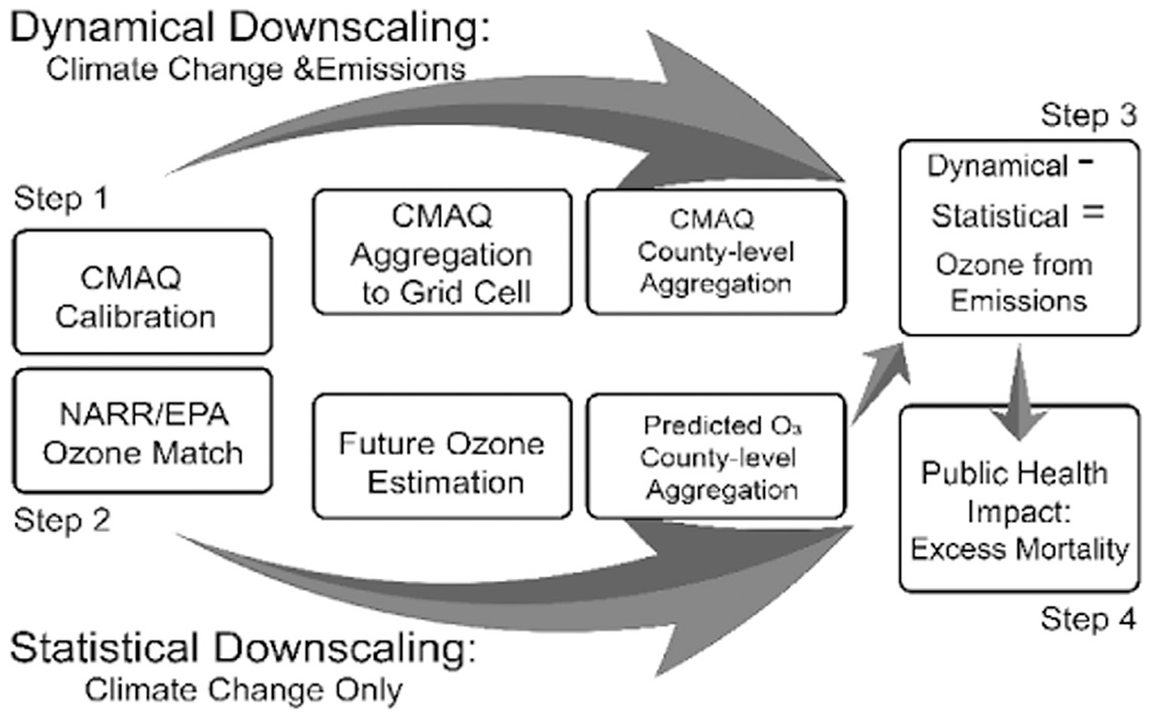
Study methods flow. Flow of study methods depicting both dynamical and statistical results. Isolation of O3 attributable to emissions accomplished by taking the difference between the two illustrated downscaling methods. Excess deaths calculated by source for climate change only, and combined climate and emissions changes. Isolation of O3 attributed to emissions is achieved by taking the difference between the two methods.
2.1. Step 1: dynamical downscaling for O3 change due to changes in climate and air pollution emissions
The Community Earth System Model version 1.0 (CESM 1.0) is a state-of-the-art global climate model developed by the National Center for Atmospheric Research (NCAR) (Gent et al., 2011). As a fully coupled earth system model, there is a total of four components in CESM(Neale et al., 2010): 1) the land surface component - Community Land Model (CLM4) (Oleson et al., 2010); 2) the ocean model and sea ice component - Parallel Ocean Program version 2 (POP2) (Smith et al., 2010) and Los Alamos National Laboratory Sea Ice Model, version 4 (CICE4) (Hunke and Lipscomb, 2008); 3) the atmospheric chemistry module - adapted from the Model for Ozone And Related chemical Tracers version 4 (MOZART-4) (Emmons et al., 2010); and 4) the bulk aerosol model (coupled to the atmospheric component Community Atmosphere Model, CAM4), referred to as CAM-Chem (Emmons et al., 2010; Lamarque et al., 2005). More details regarding the configurations of CAM-Chem have been described in previous studies (Gao et al., 2013; Lamarque et al., 2012). CESM/CAM-Chem was continuously run from 2001 to 2059 under both RCP4.5 and RCP8.5 with spatial resolution of 0.9° by 1.25°.
The dynamical downscaling framework was developed to conduct high resolution simulations (12 km) at two time slices from 2001 to 2004 for the baseline historical period and 2055 to 2059 for future scenarios under RCP 4.5 and RCP 8.5 (Gao et al., 2013; Gao et al., 2012). The Weather Research and Forecasting (WRF, version 3.2.1) and the Community Multi-scale Air Quality Model (CMAQ, version 5.0) (Wong et al., 2012), were used in this study and detailed information on model configurations and dynamical downscaling technique was described in Section 2 and 3 of Gao et al. (2013). Meteorological parameters such as hourly surface temperature, surface relative humidity, precipitation, zonal (U) and meridional (V) wind, planetary boundary layer height and pressure were generated by the WRF model whereas air pollutant concentrations such as O3 was simulated from CMAQ (Skamarock and Klemp, 2008). The historical emissions (2001–2004) were based on US EPA’s National Emission Inventory, whereas the future emissions of O3 precursors were scaled based on RCP4.5 and RCP8.5, and more details can be found in Gao et al. (2013). Thus, the CESM/WRF-CMAQ system simulates O3 concentrations in the 2050s that reflect the influence of both climate change (i.e., changes in future meteorology) and changes in anthropogenic emissions at 12 km spatial resolution (IIASA, 2013). The combined effect of climate and emissions on future ozone changes was investigated in Gao et al. (2013), and this study focuses on separating the effect of climate on future ozone concentrations. The detailed method is described in Section 2.2.
We first computed differences in maximum daily average eight-hour (MDA8) O3 between the 2000s and the 2050s for each 12 km grid cell and aggregated values to the 3109 counties to obtain annual county-level changes. To reduce the bias of model simulation, we calibrated future CMAQ MDA8 O3 levels based on the ratio of observed concentrations measured by the USEPA-AQS and the results of the year-round CMAQ-modeled historic MDA8 O3 levels. A ratio method for calibration was preferred over the use of an additive bias correction. This technique was chosen primarily because, 1) the methods in this study design calculate changes between future and historical periods and an additive correction would be cancelled out, and 2) bias correction in this study is done spatially and ratio calibrations are more appropriate for capturing potential non-linearity. Each county was assigned a population-weighted centroid based on the centroids from the 2010 US Census. Using 40 km radius buffers, the five closest CMAQ points to each county centroid are identified and average O3 values were calibrated using the ratios mentioned above (Kim et al., 2015). More details about the calibration method have been described elsewhere (Wu et al., 2014).
2.2. Step 2: statistical downscaling for O3 changes due to climate change
In order to estimate changes in O3 levels between the 2050s and 2000s caused by climate change alone, we first developed a regression model to predict O3 concentrations with meteorological variables from the North America Regional Reanalysis (NARR) dataset. The NARR dataset provides the base year (2001–2004) meteorological parameters for the statistical model. NARR is produced by the National Centers for Environmental Prediction and provides a wide range of observed climate parameters over North America on a 32 km grid (NOAA/OAR/ESRL/PSD, 2013; Mesinger et al., 2006). Prior to modeling and analysis, we compared the CESM-WRF simulations against NARR values at the daily level, using a 30-day moving average. Strong correlations of key variables between the two datasets confirmed the appropriateness of combining NARR and CESM-WRF in our approach (see Supplemental Table 1). For purposes of prediction, we computed annual medians of daily mean values for temperature, relative humidity, wind speed and direction, planetary boundary layer height, surface pressure and total annual precipitation for each 32 km (NARR) and 12 km (WRF) grid. We also calculated air stagnation which is defined as a day with surface daily wind speed < 3.2 m/s, wind speed at 500 hPa < 13 m/s, and slight or no precipitation (< 0.1 mm/day) (Wang and Angell, 1999). We then linked the MDA8 O3 concentrations with the NARR meteorological data by selecting the nearest NARR cell to the closest USEPA O3 monitoring site. Model development included all sites having at least two years of data (1334 sites). In order to minimize impacts of short-term fluctuations and to focus on longer-term trends, we used a 30-day moving average window for all meteorological variables and MDA8 O3.
To establish the associations between meteorological variables and MDA8 O3, we developed a multiple linear regression (MLR) model. We included natural cubic splines of time (Julian day) to control for the long-term trend of O3 concentration (USEPA, 2013). Usage of natural cubic splines greatly improves the coefficients of determination (R2) for the model (Davis et al., 2011). The basic form of the model is as below:
| (1) |
where y is the 30 day moving-average MDA8 O3 concentration; xk is the 30 day moving-average value of the meteorological variables (temperature, relative humidity, planetary boundary height, pressure, precipitation, and two horizontal wind components); ns (time) is the natural cubic splines of time (Julian day: four degrees of freedom), and ε is model error. We fitted this model for each EPA O3 monitoring site. We matched the estimated regression coefficients (β0 and βk’s) of the MLR model with the changes in meteorological variables between the 2050s and 2000s to obtain projected changes in O3 levels. We then interpolated the site-specific O3 changes to all 3109 counties using a nearest-neighbor approach. The NARR-MLR model estimates the average annual amount of change in O3 attributable to climate change alone. We then demonstrated the appropriateness of the chosen model using a 10-fold cross validation.
2.3. Step 3: future O3 changes due to changes of air pollution emissions
In order to isolate changes in O3 concentration attributable to future air pollution emissions alone, we calculated the differences between the concentrations generated in the previous two steps. The hybrid dynamical downscaling model involving the CMAQ-simulated O3 values represents the changes in future concentration attributable to a combination of climate change and change of anthropogenic emissions (ΔO3 climate change + emissions). The statistical downscaling model, on the other hand, is an estimation of changes in concentration due to climate change alone (ΔO3 climate change). Thus, subtracting the statistical model (climate change only) from the dynamical model (climate change and emissions) we are left with an estimation of the average annual contributions (ppb) from air pollution emissions control policies alone ((ΔO3 emissions; see Eq. (2)).
| (2) |
2.4. Step 4: population health impact of future O3 changes
Population and mortality rate estimates, as well as concentration response function (CRF) coefficients are required to estimate the excess mortality (EM) due to future changes in MDA8 O3 (ALA, 2015; Post et al., 2012; Fann et al., 2012). We utilize the four population projections developed by the Integrated Climate and Land-Use Scenarios (ICLUS) project: ICLUS Al, Bl, A2 and B2. ICLUS converts the global Special Report on Emissions Scenarios (SRES) settings into county-level projections (ALA, 2015; Post et al., 2012; USEPA, 2009; Voorhees et al.,2011). The SRES A1 storyline represents a scenario of rapid development, and slow population growth, while the A2 scenario represents regional economic development and much higher fertility rates. The B1 scenario assumes similar conditions to A1, with a larger emphasis on sustainable growth and lower domestic migration. The B2 scenario includes regional growth similar to A1 with moderate population growth, and much lower migration (USEPA, 2009). A comparison between the previous SRES projections and the new RCP projections has shown that climate conditions under RCP8.5 fall between the previous SRES A1 and A2 projections and RCP4.5 closely resembles atmospheric conditions under SRES B1 (van Vuuren and Carter, 2014). Each projected population was applied to both RCP4.5 and RCP8.5 scenarios to reflect the differences between low and high emissions scenarios with varying population conditions. It is important to note that ICLUS scenarios have varying spatial resolutions due to differing projections in land and economic growth and, therefore, absolute deaths are difficult to compare across scenarios (Agency, U. S. E. P., 2017). Therefore, we chose to normalize each ICLUS scenario independently from one another in order to compare national impact and across counties within each ICLUS scenario.
For the calculation of baseline mortality incidence, we used the predicted mortality rate for the year of 2050 at county level which is available from the Environmental Benefits Mapping and Analysis Program Community Edition 1.0.8 (BenMAP-CE) developed by the US Environmental Protection Agency (USEPA, 2012). The BenMAP-CE provides county-specific mortality rates derived from projected age-specific ratios of 2050 mortality rates to 2005 mortality rates.
We based CRFs on the association between non-accidental, all-cause mortality and short-term exposure to MDA8 O3 as estimated by Bell et al. (RR = 1.0064 (95% CI: 1.0041–1.0086) per 15 ppb) (Bell et al., 2004). The estimate from Bell et al. comes from the National Morbidity, Mortality, and Air Pollution Study (NMMAPS) dataset and covers 95 major US cities (Bell et al., 2004). We estimated changes in EM at the county level using the following equation (Post et al., 2012; Fann et al., 2012):
| (3) |
where Δy is the expected number of deaths per year that may be attributed to changing air pollution levels (i.e., O3) at county i, POPi is population of county i; MRi is population mortality rate; γ is the concentration-response coefficient for MDA8 O3; and ΔCi, is the difference in concentrations of MDA8 O3 between future (2050s) and baseline (2000s) levels of MDA8 O3.
To evaluate the uncertainty of EM estimates attributable to the ranges of the CRF coefficients and mortality rates, we applied Monte Carlo simulations (10,000 random samples) for each county, assuming a normal distribution of independent county-specific means, mortality rates and standard errors of the population and concentration variables. We then estimated climate-region and national level EM estimates by summing the county-level EMs. We also estimate 95% confidence intervals (CIs) of the EMs based on the mean and standard deviation of the Monte Carlo simulations at both levels.
3. Results
3.1. Future O3 changes due to climate change
CESM/WRF simulations indicate wide spatial variations in the meteorological variables used as the future model inputs (Step 2) (Supplemental Fig. 1). Annual medians of daily mean temperature show an increase of approximately 1.2 °C and 2.3 °C across the continental US under RCP4.5 and RCP8.5, respectively, showing greater increases in the northeast, southeast, central, northwest, and southern climate regions than in the west and southwest regions (see Fig. 2A for NOAA-defined climate regions). Annual average relative humidity (RH) could increase 0.45% under RCP4.5 and 1.1% under RCP8.5, with higher increases in the Central region. Averages of planetary boundary layer height are projected to decrease by 24.0 m under RCP4.5 and 25.2 m under RCP8.5. Meridional (N/S) wind speed will decrease in most inland areas of the US under both RCPs, with highest decreases in the Northwest region. Zonal (E/W) wind speed will decrease in much of the US with some increase seen in the West and Southwest regions.
Fig. 2.
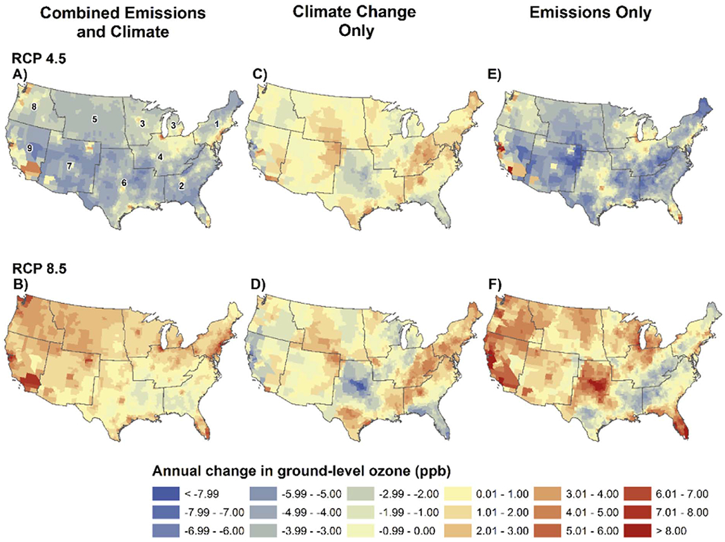
Average annual change in tropospheric O3. Changes in O3 concentrations between 2000s and 2050s. (A) O3 difference from combined climate change and emissions under RCP4.5; (B) O3 difference from combined climate change and emissions under RCP8.5; (C) O3 difference from climate change under RCP4.5; (D) O3 difference from climate change under RCP8.5; (E) O3 difference from emissions only under RCP4.5; and (F) O3 difference from emissions only under RCP8.5. Numbers represent US Climate Regions as defined by the National Climatic Data Center: 1. Northeast, 2. Southeast, 3. East North Central, 4. Central, 5. West North Central, 6. South, 7. Southwest, 8. Northwest, and 9. West (NCDC/NOAA, 2013).
Fig. 2 depicts the MLR-estimated change in annual mean MDA8 O3 concentrations (2050s vs. 2000s) for both RCP4.5 and RCP8.5. For all 1334 O3 monitoring sites, the MLR model performs well with relatively high R2 values (average R2 = 0.74). Fig. 2C and D show the MDA8 O3 changes between the 2000s and the 2050s from the statistical down-scaling model. Climate change alone appears to cause some increase in MDA8 O3 average annual (ppb) concentration in most of the continental US except for some counties in the West and South regions. Overall, increases in MDA8 O3 due to climate change is projected to be 0.34 ppb (std. error 0.03) and 0.50 ppb (std. error: 0.04) under RCP4.5 and RCP8.5, respectively. The model performance was confirmed using a 10-fold cross validation comparing the results of the study model to the results from a series of models configured using both training and testing data. The validation resulted in < 1% difference in root mean square error (RMSE) (~0.00001%).
3.2. Future O3 levels due to climate change and changes in emissions
As simulated by the CESM/WRF-CMAQ system, modest climate change and strict emissions control under RCP4.5 result in a nationwide decrease in future MDA8 O3 levels (on average 2.85 ppb, std. error: 0.03) except in a few large urban centers including Los Angeles, Chicago, and New York (Fig. 2A). These hotspots of high O3 under RCP4.5 are likely caused by NOx decreases in large urban areas, resulting in reduced O3 titration and higher concentrations of O3 (Gao et al., 2013). Under RCP8.5, national mean O3 level is projected to increase by ~ 1.33 ppb annually (std. error: 0.03, Fig. 2B). With greater temperature rise, climate change only caused O3 levels to increase in more regions under RCP8.5 than under RCP4.5, but the spatial patterns of O3 changes are similar under these two scenarios (Fig. 2D).
3.3. Future O3 change due to changes of air pollution emissions
Under RCP4.5, average national MDA8 O3 due to emissions alone decreases by 3.19 ppb (std. error: 0.04, Fig. 2E). Comparing Fig. 2C and E, it is clear that the O3 reduction due to the assumed lower precursor emissions outweighs the O3 increase due to higher temperature under RCP4.5. On the other hand, changes in future emissions alone under RCP8.5 would cause O3 levels to increase in the US except in the mid-Atlantic and Southeastern region (Fig. 2F). Despite the emission reduction of O3 precursors across all RCPs (including CO, NOx and MVOCs), nationally averaged MDA8 O3 may increase by 0.93 ppb (std. error: 0.05) in the 2050s under RCP8.5.
3.4. Population health impact of future O3
Fig. 3 displays the annual average, population-normalized county estimates for excess mortality in 2055–2059 for the ICLUS A2 scenario (high population growth) for both RCP4.5 and RCP8.5 per 100,000 persons. Emissions sources appear to play a significant role, especially in RCP8.5, with large increases in O3-related mortality for much of the West, Midwest, and Eastern US. Table 1 shows the estimated O3-related excess deaths by climate region for the ICLUS A2 scenario under RCP4.5 and RCP8.5. The highest excess deaths are found from emissions-only sources (compared to climate change only sources) under RCP8.5 with the West, Southeast, and Northeast regions showing the largest impact. Similar patterns are found for other ICLUS population scenarios and data can be found in Supplemental Tables 2 and 3.
Fig. 3.
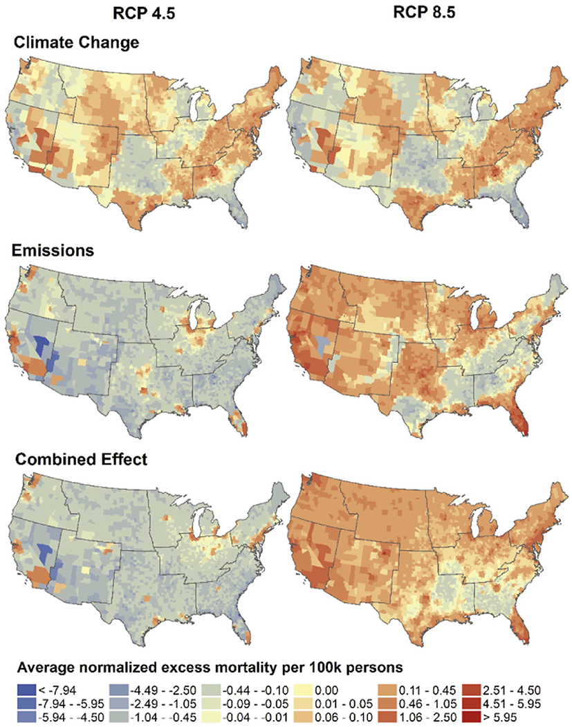
Change in mortality: RCPs 4.5 and 8.5 using ICLUS A2 Scenario. Annual averaged, county-level excess mortality normalized by population. RCP4.5 (low emissions scenario) and RCP8.5 (high emissions scenario) results displayed by contributing source (combined effects, climate change and anthropogenic emissions). The combined effects represent the effects of both climate change and emissions.
Table 1.
Short term excess mortality under the ICLUS A2 population scenario. Projected excess deaths using ICLUS A2 population scenarios attributable to climate change only, anthropogenic emissions only, and combined effects of both climate change and emissions for 2050s from baseline 2000s by US climatic region. (SE: standard error).
| Climate change only |
Emissions control only |
Combined effect |
||||
|---|---|---|---|---|---|---|
| Region | RCP4.5 | RCP8.5 | RCP4.5 | RCP8.5 | RCP4.5 | RCP8.5 |
| National | 72 | 47 | −41 | 2167 | 50 | 2217 |
| (SE = 456) | (SE = 525) | (SE = 1037) | (SE = 1386) | (SE = 615) | (SE = 900) | |
| Northeast | 204 | 330 | − 2 | 365 | 208 | 678 |
| (SE = 12) | (SE = 17) | (SE = 28) | (SE = 43) | (SE = 40) | (SE = 59) | |
| Southeast | −47 | −100 | −186 | 405 | −237 | 298 |
| (SE = 10) | (SE = 17) | (SE = 14) | (SE = 35) | (SE = 5) | (SE = 19) | |
| East North Central | −18 | −35 | 22 | 161 | 4 | 126 |
| (SE = 1) | (SE = 1) | (SE = 1) | (SE = 3) | (SE = 1) | (SE = 3) | |
| Central | 76 | 87 | −42 | 161 | 30 | 239 |
| (SE = 4) | (SE = 4) | (SE = 7) | (SE = 12) | (SE = 11) | (SE = 15) | |
| West North Central | 5 | 5 | −20 | 9 | −15 | 13 |
| (SE = 1) | (SE = 1) | (SE = 1) | (SE = 1) | (SE = 1) | (SE = 1) | |
| South | −11 | −13 | −80 | 169 | −91 | 152 |
| (SE = 3) | (SE = 3) | (SE = 3) | (SE = 6) | (SE = 4) | (SE = 6) | |
| Southwest | 20 | 18 | −71 | 98 | −52 | 114 |
| (SE = 7) | (SE = 7) | (SE = 7) | (SE = 15) | (SE = 3) | (SE = 13) | |
| Northwest | −12 | −5 | 46 | 122 | 34 | 112 |
| (SE = 2) | (SE = 2) | (SE = 6) | (SE = 8) | (SE = 5) | (SE = 9) | |
| West | −143 | −170 | 292 | 678 | 165 | 475 |
| (SE = 154) | (SE = 182) | (SE = 355) | (SE = 468) | (SE = 199) | (SE = 287) | |
Fig. 4 highlights the state of California—an area of the US known for its pollution and related health issues. Shown together are the county-level O3 and mortality results for RCP8.5. Hot spots of O3 concentration increases and O3-related EM can be seen in areas surrounding the San Francisco Bay and Los Angeles County. Notably, changes in O3 concentration due to emissions appear to be highest in counties such as Los Angeles, Monterey, Orange, and San Joaquin. Meanwhile, O3 concentration due to emissions appears to be lowest in the upper counties and central valley. On the whole, under ICLUS A2 and RCP8.5, O3-related EM due to climate change alone may increase by 180 deaths/year (std. error: 23.92) while under RCP4.5, 110 (std. error: 21.63) excess deaths may be expected due to climate change. However, emissions may have a greater impact on estimated excess mortality in California exhibiting an increase of approximately 315 (std. error: 21.21) deaths under RCP8.5. Under RCP4.5 excess deaths due to emissions can be expected to increase at much lower rates with only 87 (std. error: 8.98) deaths/year in the 2050s. In predictions including both sources, excess deaths under RCP8.5 for the state of California may exceed 486 deaths/year (std. error: 44.13) while scenarios using RCP4.5 predict lower increases of 230 deaths/year (std. error: 30.55).
Fig. 4.
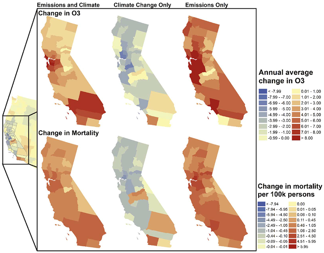
Sample of results: California case study. Annual averaged, county-level changes In O3 and excess mortality normalized by population depicted for the state of California under RCP8.5.
4. Discussion
Our results point to significant differences in the contributions of climate and emissions mitigation to future O3. Under both RCP scenarios, future emissions control policy will likely have a substantial impact on O3 levels and its associated health effects. Our hybrid downscaling approach suggests that changes in emissions may be the source of the main incongruities between RCP4.5 and RCP8.5. Thus, while climate change alone may cause some adverse health effects due to poorer air quality, substantial and more immediate health benefits may be achieved by emission mitigation of O3 precursors regardless of changing climate conditions especially under RCP8.5.
In all RCPs, most emissions of O3 precursors are expected to decrease in the US due to nearly worldwide implementation of stricter environmental policies. However, the results under RCP8.5 suggest a rise in future O3 concentrations. It is important to note that, with the climate change effect removed, the predictions still include background O3 conditions. As is explained in Gao et al. (2013), the O3 changes in RCP8.5 primarily occurs in spring and winter, especially over the western US, due to increases in global methane emissions (60% by the end of 2050s). In summer and fall, particularly over the eastern US, the increase of methane emissions is offset by the large reduction in anthropogenic VOC and NOx emissions, leading to decrease of O3 concentrations (Gao et al., 2013). Increases of O3 in RCP 8.5 were also found across a majority of the troposphere in Young et al. (2013), which attributes the higher ozone concentration to large increase of methane and greater stratospheric influx (Young et al., 2013). The tropospheric ozone increase in RCP 8.5 was shown to enhance background ozone, further impacting regional modeling results through the boundary conditions. This enhanced background ozone can lead to elevated spring ozone in the western US and has also been documented by Lin et al. (2012).
Several recent studies have demonstrated findings comparable to our results regarding the ozone changes in RCP 4.5 and RCP 8.5 (Clifton et al., 2014; Rieder et al., 2015; Yahya et al., 2017). In particular, as is shown in Gao et al. (2013; Fig. 5c), the ozone increases largely disappear when the boundary conditions were cleaner and methane emission increases were removed in RCP 8.5. The effect of global background ozone increase on regional downscaling results through boundary conditions was further shown by a more recent sensitivity study (Yahya et al., 2017, Fig. 7i vs. Figure 7iii), showing clearly that the high ozone boundary conditions inherited from global models under RCP 8.5 contributed to majority of the ozone increases in US in regional model results (Yahya et al., 2017). Thus, the combination of global background ozone increases and methane emission increases may be the main contributing factor for increases in O3 and O3-related EM under RCP8.5. Researchers have evaluated and proposed that the control of methane emissions may be an efficient way to reduce both tropospheric O3 and radiative forcing (Nolte et al., 2008; West and Fiore, 2005; West et al., 2013).
It is important to note that the estimated EM attributable to O3 changes vary significantly, showing both negative and positive results by region, as seen in Table 1 and Supplemental Tables 2 and 3. Additionally, relatively high standard deviations are captured for most of the regional predictions. These reflect the varying EM from county-to-county within the regions. Further uncertainty is introduced with the CRF values which have been derived from short-term O3 exposure (robust long-term estimates remain unavailable in the literature) with the assumption that county-specific CRF coefficients are normally distributed. However, despite these limitations, the high-resolution hybrid downscaling system presented here allows the examination of EM at the county level, which is a major strength of our current study. As expected, county-level O3-related EM is high in counties with higher populations. However, US counties, in general, stand to benefit from emission changes under RCP4.5 scenarios.
Since climate change can have important ramifications in California such as more severe and frequent wildfires and air pollution episodes, it has been the focus of extensive air pollution and climate research (Mahmud et al., 2008; Fujita et al., 2016; He et al., 2016; Fujita et al., 2013). For example, Mahmud et al. performed statistical downscaling methods in the state of California using temperature data from the National Center for Atmospheric Research (NCAR) Reanalysis and 1-hour maximum O3 values from two ground monitors (Mahmud et al., 2008). The air temperature data have a coarse spatial resolution (2.5° × 4°), which makes it difficult to be directly associated with daily O3 levels. Instead, linear regression models were developed between 850-hPa air temperature and quartiles of O3 concentrations, posing an obstacle when linking O3 exposure with population-specific concentration-response functions. Fujita et al., while using a high resolution (5 km) chose to utilize a chemical box model in which only one parameter was allowed to change at a time. While the methods vary significantly from those used in our study, the general trend of increasing O3 and emissions is still evident (Fujita et al., 2013). Additionally, He et al. designed a study at a relatively low resolution (30 km) using multiple scenarios: climate change only, emissions only, and a boundary effect. Using CMAQ and the Sparse Matrix Operator Kernel Emissions Model (SMOKE), these scenarios were based on SRES A1B and A1FI. Generally, A1B is similar to the RCP4.5 scenario used in our study in terms of greenhouse gas emission increases and anthropogenic emission decrease, however, A1FI is very different from RCP8.5. In A1fi, all anthropogenic emissions are projected to increase. In RCP8.5, VOC/NOx is actually projected to decrease with large increases in methane leading to consequent rises in ozone levels (He et al., 2016). Taken together, overall conclusions of these case studies are consistent with our results, but the use of hybrid downscaling and the updated RCP scenarios strengthens our current study and lends more insight into the nuances of future ozone changes.
While we have sought to improve on previous methods, some limitations remain. Uncertainties may lie in the estimation of the future mortality rate, CRF, population projection, the potential effect of interactions between temperature and O3, and O3 concentration predictions (Brown et al., 2014; Chang et al., 2014; Deser et al., 2012; Henneman et al., 2017; Meehl and Stocker, 2007). We attempt to account for some uncertainty by evaluating EM estimates using a robust Monte Carlo method. We acknowledge that other modeling frameworks have been proposed, however, we deemed our approach reasonable due to sufficient high model performance (Chang et al., 2014; Henneman et al., 2017). Exploration of additional techniques, though a future direction of study, was beyond the scope of this analysis. Another drawback lies in the cubic splines of time used in the model as they may underestimate the contribution of climate change to O3 concentrations due to the removal of long-term trends. Additionally, the use of county-level resolution, while more precise than previous studies, may still cause some loss in detail of future O3 predictions. However, it is necessary to keep the resolution of this data consistent with the resolution of the health data for analysis purposes (i.e., health data kept at county level for privacy protection). Future efforts to improve on this analysis could include enhancements in pollutant data collection locations, the addition of co-pollutant effects, and the effects of pollutants on human morbidity.
5. Conclusions
The results of this study demonstrate that potential increases in premature death and in adverse health effects of climate change-induced O3 increases in the US may be substantially offset by the effect of emission reductions planned under RCP4.5. However, even with the reduction of O3 precursors, O3-related excess mortality may still increase in the US, due to increases in methane emissions under RCP8.5. Thus, with responsible emissions policy, the effects of emission reduction of O3 precursors is poised to significantly offset the adverse health effects of O3 due to climate change. To prevent adverse health effects of this potential driver, it is important to continue to intensify mitigation efforts towards both GHGs and O3 precursor emissions. These efforts are likely to avoid great cost to human health and quality of life.
Supplementary Material
Acknowledgements
This study was supported by the EPA STAR Program (Grant NO. 83586901), the Centers for Disease Control and Prevention (Grant No. 5 U01 EH000405), the National Institutes of Health (Grant No. 1R21ES020225), and the National Science Foundation through TeraGrid (TG-ATM110009 and UT-TENN0006). The Oak Ridge Leadership Computing Facility at the Oak Ridge National Laboratory supported by the Office of Science of the US Department of Energy (DEAC05-00OR22725) was used for the climate and air pollution model simulations.
Abbreviations:
- O3
ozone
- RCPs
Representative Concentration Pathways
- NMVOC
non-methane volatile organic carbon
- NOx
nitrogen oxides
- GCMs
global climate models
- SRES
Special Report on Emissions Scenarios
- GHGs
greenhouse gases
- CESM
Community Earth System Model
- NCAR
National Center for Atmospheric Research
- WRF
Weather Research and Forecasting model
- CMAQ
Community Multi-scale Air Quality model
- CAM-Chem
Community Atmosphere Model w/ chemistry
- MDA8 O3
maximum daily average eight-hour ozone
- ICLUS
Integrated Climate and Land-Use Scenarios
Footnotes
Conflicts of interest
The authors of this manuscript have no competing associations or conflicts of interest pertaining to this study.
Appendix A. Supplementary data
Supplementary data to this article can be found online at http://dx.doi.org/10.1016/j.envint.2017.08.001.
References
- Agency, U. S. E. P., 2017. Updates to the Demographic and Spatial Allocation Models to Produce Integrated Climate and Land Use Scenarios (ICLUS) (Final Report, Version 2). Washington, D.C. . [Google Scholar]
- ALA, 2015. A. L. A. State of the Air 2015. American Lung Association, Chicago, IL. [Google Scholar]
- Bell ML, McDermott A, Zeger SL, Samet JM, Dominici F, 2004. Ozone and short-term mortality in 95 US urban communities, 1987–2000. JAMA 292, 2372–2378. 10.1001/jama.292.19.2372. [DOI] [PMC free article] [PubMed] [Google Scholar]
- Bell ML, Dominici F, Samet JM, 2005. A meta-analysis of time-series studies of ozone and mortality with comparison to the national morbidity, mortality, and air pollution study. Epidemiology 16, 436–445. 10.1097/01.ede.0000165817.40152.85. [DOI] [PMC free article] [PubMed] [Google Scholar]
- Bell ML, et al. , 2007. Climate change, ambient ozone, and health in 50 US cities. Clim. Chang. 82, 61–76. 10.1007/s10584-006-9166-7. [DOI] [Google Scholar]
- Bernard SM, Samet JM, Grambsch A, Ebi KL, Romieu I, 2001. The potential impacts of climate variability and change on air pollution-related health effects in the United States. Environ. Health Perspect. 109, 199–209. 10.2307/3435010. [DOI] [PMC free article] [PubMed] [Google Scholar]
- Brown SJ, Murphy JM, Sexton DMH, Harris GR, 2014. Climate projections of future extreme events accounting for modelling uncertainties and historical simulation biases. Clim. Dyn. 43, 2681–2705. 10.1007/s00382-014-2080-1. [DOI] [Google Scholar]
- Camalier L, Cox W, Dolwick P, 2007. The effects of meteorology on ozone in urban areas and their use in assessing ozone trends. Atmos. Environ. 41, 7127–7137. 10.1016/j.atmosenv.2007.04.061. [DOI] [Google Scholar]
- Chang HH, Hao H, Sarnat SE, 2014. A statistical modeling framework for projecting future ambient ozone and its health impact due to climate change. Atmos. Environ. (Oxford, England: 1994) 89, 290–297. 10.1016/j.atmosenv.2014.02.037. [DOI] [PMC free article] [PubMed] [Google Scholar]
- Clifton OE, Fiore AM, Correa G, Horowitz LW, Naik V, 2014. Twenty-first century reversal of the surface ozone seasonal cycle over the northeastern United States. Geophys. Res. Lett. 41, 7343–7350. 10.1002/2014g1061378. [DOI] [Google Scholar]
- Cox WM, Chu SH, 1996. Assessment of interannual ozone variation in urban areas from a climatological perspective. Atmos. Environ. 30, 2615–2625. 10.1016/1352-2310(95)00346-0. [DOI] [Google Scholar]
- Davis J, Cox W, Reff A, Dolwick P, 2011. A comparison of CMAQ-based and observation-based statistical models relating ozone to meteorological parameters. Atmos. Environ. 45, 3481–3487. 10.1016/j.atmosenv.2010.12.060. [DOI] [Google Scholar]
- Dawson JP, Adams PJ, Pandis SN, 2007. Sensitivity of ozone to summertime climate in the eastern USA: a modeling case study. Atmos. Environ. 41, 1494–1511. 10.1016/j.atmosenv.2006.10.033. [DOI] [Google Scholar]
- Deser C, Phillips A, Bourdette V, Teng HY, 2012. Uncertainty in climate change projections: the role of internal variability. Clim. Dyn. 38, 527–546. 10.1007/S00382-010-0977-x. [DOI] [Google Scholar]
- Diem JE, 2003. A critical examination of ozone mapping from a spatial-scale perspective. Environ. Pollut. 125, 369–383. 10.1016/s0269-7491(03)00110-6. [DOI] [PubMed] [Google Scholar]
- Emmons LK, et al. , 2010. Description and evaluation of the Model for Ozone and Related chemical Tracers, version 4 (MOZART-4). Geosci. Model Dev. 3, 43–67. [Google Scholar]
- Fann N, et al. , 2012. Estimating the national public health burden associated with exposure to ambient PM2.5 and ozone. Risk Anal. 32, 81–95. 10.1111/j.1539-6924.2011.01630.x. [DOI] [PubMed] [Google Scholar]
- Fiore A, Naik V, Leibensperger E, 2015. Air quality and climate connections (vol 65, pg 645-685, 2015). J. Air Waste Manage. Assoc. 65, 1159. 10.1080/10962247.2015.1059177. [DOI] [PubMed] [Google Scholar]
- Fujita EM, Campbell DE, Stockwell WR, Lawson DR, 2013. Past and future ozone trends in California’s South Coast Air Basin: reconciliation of ambient measurements with past and projected emission inventories. J. Air Waste Manage. Assoc. 63, 54–69. 10.1080/10962247.2012.735211. [DOI] [PubMed] [Google Scholar]
- Fujita EM, et al. , 2016. Projected ozone trends and changes in the ozone-precursor relationship in the South Coast Air Basin in response to varying reductions of precursor emissions. J. Air Waste Manage. Assoc. 66, 201–214. 10.1080/10962247.2015.1106991. [DOI] [PubMed] [Google Scholar]
- Gao Y, Fu JS, Drake JB, Liu Y, Lamarque JF, 2012. Projected changes of extreme weather events in the eastern United States based on a high resolution climate modeling system. Environ. Res. Lett. 7. 10.1088/1748-9326/7/4/044025. [DOI] [Google Scholar]
- Gao Y, Fu JS, Drake JB, Lamarque JF, Liu Y, 2013. The impact of emission and climate change on ozone in the United States under representative concentration pathways (RCPs). Atmos. Chem. Phys. 13, 9607–9621. 10.5194/acp-13-9607-2013.. [DOI] [PMC free article] [PubMed] [Google Scholar]
- Gent PR, et al. , 2011. The community climate system model version 4. J. Clim. 24, 4973–4991. 10.1175/2011jcli4083.1. [DOI] [Google Scholar]
- Gryparis A, et al. , 2004. Acute effects of ozone on mortality from the “air pollution and health: a European approach” project. Am. J. Respir. Crit. Care Med. 170, 1080–1087. 10.1164/rccm.200403-333OC. [DOI] [PubMed] [Google Scholar]
- He H, Liang XZ, Lei H, Wuebbles DJ, 2016. Future US ozone projections dependence on regional emissions, climate change, long-range transport and differences in modeling design. Atmos. Environ. 128, 124–133. 10.1016/j.atmosenv.2015.12.064. [DOI] [Google Scholar]
- Henneman LR, et al. , 2017. Accountability assessment of regulatory impacts on ozone and PM2.5 concentrations using statistical and deterministic pollutant sensitivities. Air Qual. Atmos. Health 1–17. 10.1007/s11869-017-0463-2.28111595 [DOI] [Google Scholar]
- Hunke EC, Lipscomb WH, 2008. CICE: The Los Alamos Sea Ice Model, Documentation and Software, Version 4.0. Los Alamos National Laboratory Tech. Rep. [Google Scholar]
- IIASA, 2013. I. I. f. A. S. A. RCP Database Version 2.0. http://tntcat.iiasa.ac.at:8787/RcpDb/dsd?Action=htmlpage&page=welcome.
- IPCC, 2013. In: Stocker TF (Ed.), Climate Change 2013: The Physical Science Basis. Contribution of Working Group I to the Fifth Assessment Report of the Intergovernmental Panel on Climate Change. Cambridge University Press, pp. 1–30 Ch. SPM. [Google Scholar]
- Jackson JE, et al. , 2010. Public health impacts of climate change in Washington State: projected mortality risks due to heat events and air pollution. Clim. Chang. 102, 159–186. 10.1007/s10584-010-9852-3. [DOI] [Google Scholar]
- Jacob DJ, Winner DA, 2009. Effect of climate change on air quality. Atmos. Environ. 43, 51–63. 10.1016/j.atmosenv.2008.09.051. [DOI] [Google Scholar]
- Jerrett M, et al. , 2009. Long-term ozone exposure and mortality. N. Engl. J. Med. 360, 1085–1095. 10.1056/NEJMoa0803894. [DOI] [PMC free article] [PubMed] [Google Scholar]
- Kim YM, et al. , 2015. Spatially resolved estimation of ozone-related mortality in the United States under two representative concentration pathways (RCPs) and their uncertainty. Clim. Chang. 128, 71–84. 10.1007/s10584-014-1290-1. [DOI] [PMC free article] [PubMed] [Google Scholar]
- Lamarque JF, et al. , 2005. Response of a coupled chemistry-climate model to changes in aerosol emissions: global impact on the hydrological cycle and the tropospheric burdens of OH, ozone, and NOx. Geophys. Res. Lett. 32. 10.1029/2005gl023419. [DOI] [Google Scholar]
- Lamarque JF, et al. , 2012. CAM-chem: description and evaluation of interactive atmospheric chemistry in the Community Earth System Model. Geosci. Model Dev. 5, 369–411. 10.5194/gmd-5-369-2012. [DOI] [Google Scholar]
- Levy JI, Chemerynski SM, Sarnat JA, 2005. Ozone exposure and mortality - an empiric Bayes metaregression analysis. Epidemiology 16, 458–468. 10.1097/01.ede.0000165820.08301.b3. [DOI] [PubMed] [Google Scholar]
- Lin MY, et al. , 2012. Springtime high surface ozone events over the western United States: quantifying the role of stratospheric intrusions. J. Geophys. Res.-Atmos. 117. 10.1029/2012jd018151. [DOI] [Google Scholar]
- Mahmud A, Tyree M, Cayan D, Motallebi N, Kleeman MJ, 2008. Statistical downscaling of climate change impacts on ozone concentrations in California. J. Geophys. Res.-Atmos. 113. 10.1029/2007jd009534. [DOI] [Google Scholar]
- Meehl GA, Stocker TF, 2007. Global Climate Projections. Cambridge Univ Press. [Google Scholar]
- Mesinger F, et al. , 2006. North American regional reanalysis. Bull. Am. Meteorol. Soc. 87, 343–360. 10.1175/bams-87-3-343. [DOI] [Google Scholar]
- Moss RH, et al. , 2010. The next generation of scenarios for climate change research and assessment. Nature 463, 747–756. 10.1038/nature08823. [DOI] [PubMed] [Google Scholar]
- Murphy J, 2000. Predictions of climate change over Europe using statistical and dynamical downscaling techniques. Int. J. Climatol. 20, 489–501. . [DOI] [Google Scholar]
- NCDC/NOAA, 2013. U.S. Climate Regions, http://www.ncdc.noaa.gov/monitoring-references/maps/us-climate-regions.php.
- Neale RB, et al. , 2010. Description of the NCAR Community Atmosphere Model (CAM 4.0), NCAR Tech. Note NCAR/TN-XXX+STR (Draft). National Center for Atmospheric Research, Boulder, Colorado. [Google Scholar]
- NOAA/OAR/ESRL/PSD, 2013. National Centers for Environmental Prediction (NCEP) North American Regional Reanalysis (NARR). http://esrl.noaa.gov/psd/data/gridded/data.narr.monolevel.html.
- Nolte CG, Gilliland AB, Hogrefe C, Mickley LJ, 2008. Linking global to regional models to assess future climate impacts on surface ozone levels in the United States. J. Geophys. Res.-Atmos. 113. 10.1029/2007jd008497. [DOI] [Google Scholar]
- Oleson KW, et al. , 2010. Technical Description of Version 4.0 of the Community Land Model (CLM). National Center for Atmospheric Research, Boulder, Colorado. [Google Scholar]
- Post ES, et al. , 2012. Variation in estimated ozone-related health impacts of climate change due to modeling choices and assumptions. Environ. Health Perspect. 120, 1559–1564. 10.1289/ehp.1104271. [DOI] [PMC free article] [PubMed] [Google Scholar]
- Rieder HE, Fiore AM, Horowitz LW, Naik V, 2015. Projecting policy-relevant metrics for high summertime ozone pollution events over the eastern United States due to climate and emission changes during the 21st century. J. Geophys. Res.-Atmos. 120, 784–800. 10.1002/2014jd022303. [DOI] [Google Scholar]
- Skamarock WC, Klemp JB, 2008. A time-split nonhydrostatic atmospheric model for weather research and forecasting applications. J. Comput. Phys. 227, 3465–3485. 10.1016/j.jcp.2007.01.037. [DOI] [Google Scholar]
- Smith R, et al. , 2010. The Parallel Ocean Program (POP) Reference Manual Ocean Component of the Community Climate System Model (CCSM) and Community Earth System Model (CESM). Los Alamos National Laboratory Boulder, Colorado. [Google Scholar]
- Stieb DM, Szyszkowicz M, Rowe BH, Leech JA, 2009. Air pollution and emergency department visits for cardiac and respiratory conditions: a multi-city time-series analysis. Environ. Health 8. 10.1186/1476-069x-8-25. [DOI] [PMC free article] [PubMed] [Google Scholar]
- Tagaris E, et al. , 2009. Potential impact of climate change on air pollution-related human health effects. Environ. Sci. Technol. 43, 4979–4988. 10.1021/es803650w. [DOI] [PubMed] [Google Scholar]
- USEPA, 2009. U. S. E. P. A. Land-use Scenarios: National-scale Housing-density Scenarios Consistent With Climate Change Storylines (Final Report). Washington, DC: . [Google Scholar]
- USEPA, 2012. U. S. E. P. A. BenMap: Environmental Benefits Mapping and Analysis Program: User’s Manual Appendices. USEPA, Research Triangle Park, NC. [Google Scholar]
- USEPA, 2013. U. S. E. P. A. Integrated Science Assessment for Ozone and Related Photochemical Oxidants. Research Triangle Park, NC. [Google Scholar]
- van Vuuren DP, Carter TR, 2014. Climate and socio-economic scenarios for climate change research and assessment: reconciling the new with the old. Clim. Chang. 122, 415–429. 10.1007/s10584-013-0974-2. [DOI] [Google Scholar]
- van Vuuren DP, et al. , 2011. The representative concentration pathways: an overview. Clim. Chang. 109, 5–31. 10.1007/s10584-011-0148-z. [DOI] [Google Scholar]
- Voorhees AS, et al. , 2011. Climate change-related temperature impacts on warm season heat mortality: a proof-of-concept methodology using BenMAP. Environ. Sci. Technol. 45, 1450–1457. 10.1021/es102820y. [DOI] [PubMed] [Google Scholar]
- Wang J, Angell J, 1999. Air Stagnation Climatology for the United States. NOA/Air Resource Laboratory Atlas No. 1. [Google Scholar]
- West JJ, Fiore AM, 2005. Management of tropospheric ozone by reducing methane emissions. Environ. Sci. Technol. 39, 4685–4691. 10.1021/es048629f. [DOI] [PubMed] [Google Scholar]
- West JJ, et al. , 2013. Co-benefits of mitigating global greenhouse gas emissions for future air quality and human health. Nat. Clim. Chang. 3, 885–889. 10.1038/nclimate2009. [DOI] [PMC free article] [PubMed] [Google Scholar]
- Wong DC, et al. , 2012. WRF-CMAQ two-way coupled system with aerosol feedback: software development and preliminary results. Geosci. Model Dev. 5, 299–312. 10.5194/gmd-5-299-2012. [DOI] [Google Scholar]
- Wu JY, et al. , 2014. Estimation and uncertainty analysis of impacts of future heat waves on mortality in the Eastern United States. Environ. Health Perspect. 122, 10–16. 10.1289/ehp.1306670. [DOI] [PMC free article] [PubMed] [Google Scholar]
- Yahya K, Campbell P, Zhang Y, 2017. Decadal application of WRF/chem for regional air quality and climate modeling over the U.S. under the representative concentration pathways scenarios. Part 2: current vs. future simulations. Atmos. Environ. 152, 584–604. 10.1016/j.atmosenv.2016.12.028. [DOI] [Google Scholar]
- Young PJ, et al. , 2013. Pre-industrial to end 21st century projections of tropospheric ozone from the Atmospheric Chemistry and Climate Model Intercomparison Project (ACCMIP). Atmos. Chem. Phys. 13, 2063–2090. 10.5194/acp-13-2063-2013. [DOI] [Google Scholar]
Associated Data
This section collects any data citations, data availability statements, or supplementary materials included in this article.