Designing Single- and Multiple-Shell Sampling Schemes for Diffusion MRI Using Spherical Code

Abstract

In diffusion MRI (dMRI), determining an appropriate sampling scheme is crucial for acquiring the maximal amount of information for data reconstruction and analysis using the minimal amount of time. For single-shell acquisition, uniform sampling without directional preference is usually favored. To achieve this, a commonly used approach is the Electrostatic Energy Minimization (EEM) method introduced in dMRI by Jones et al. However, the electrostatic energy formulation in EEM is not directly related to the goal of optimal sampling-scheme design, i.e., achieving large angular separation between sampling points. A mathematically more natural approach is to consider the Spherical Code (SC) formulation, which aims to achieve uniform sampling by maximizing the minimal angular difference between sampling points on the unit sphere. Although SC is well studied in the mathematical literature, its current formulation is limited to a single shell and is not applicable to multiple shells. Moreover, SC, or more precisely continuous SC (CSC), currently can only be applied on the continuous unit sphere and hence cannot be used in situations where one or several subsets of sampling points need to be determined from an existing sampling scheme. In this case, discrete SC (DSC) is required. In this paper, we propose novel DSC and CSC methods for designing uniform single-/multi-shell sampling schemes. The DSC and CSC formulations are solved respectively by Mixed Integer Linear Programming (MILP) and a gradient descent approach. A fast greedy incremental solution is also provided for both DSC and CSC. To our knowledge, this is the first work to use SC formulation for designing sampling schemes in dMRI. Experimental results indicate that our methods obtain larger angular separation and better rotational invariance than the generalized EEM (gEEM) method currently used in the Human Connectome Project (HCP).

1. Introduction

Diffusion MRI (dMRI) is a unique technique for exploring the underlying tissue properties of white matter in the human brain. A central problem in dMRI is to reconstruct the MR signal attenuation E(q) from a limited number of measurements in the q-space and to estimate some meaningful quantities such as the Ensemble Average Propagator (EAP) and the Orientation Distribution Function (ODF). An effective q-space sampling scheme is critical for the acquisition of maximum information with minimum time cost. Since white matter fascicles traverse the brain in a wide range of directions, a uniform sampling scheme with no directional preference is often preferred [1].

In the last decade, two approaches have been widely used for designing sampling schemes for single-shell acquisition. The first approach involves tessellation of a unit sphere using basic shapes such as the icosahedron. Using such a spherical tessellation approach, however, one is unable to generate a sampling scheme with an arbitrary number of sample points. The second approach is the Electrostatic Energy Minimization (EEM) method, which was introduced in dMRI by Jones et al. [1]. Some best known solutions to the EEM problem have been collected in CAMINO [2]. EEM was also recently generalized for multi-shell sampling [3,4] with staggered samples in different shells and has been adopted in the Human Connectome Project (HCP) [5]. However, the electrostatic energy formulation in EEM is not directly related to the goal of sampling scheme design, which is to maximize the angular separation between sampling points, and it is still unknown why electrostatic energy matters in dMRI reconstruction.

A good sampling scheme should have large angular separation such that the reconstruction has large angular resolution and good rotational invariance. Thus a mathematically more natural way for sampling scheme design is to maximize the minimal angular difference between sampling points, i.e., covering radius, on a unit sphere. Determining such point configuration is essentially the Spherical Code (SC) problem¹, and there are a collection of best known solutions for the SC problem in ${\mathbb{S}}^2$ [6]². Although SC is well studied in the mathematical literature, its current formulation is limited to a single shell and is not applicable to multiple shells. Moreover, SC, or more precisely continuous SC (CSC), currently can only be applied on the continuous unit sphere and hence cannot be used in situations where several subsets of sampling points need to be determined from an existing sampling scheme. In this case, discrete SC (DSC) is required, where the solution space is discrete and determined by a set of predetermined sampling points.

In this paper, we propose novel CSC and DSC methods for designing single-/multi-shell sampling schemes. We propose a greedy incremental estimation for rapid generation of solutions to the DSC and CSC problems, a Mixed Integer Linear Programming (MILP) method to solve the DSC problem, and a Riemannian gradient descent method to solve the CSC problem. Experimental results indicate that the proposed methods are capable of yielding larger covering radius and better rotational invariance than the state-of-the-art generalized EEM (gEEM) method currently used in the HCP [4,5].

2. Designing Sampling Scheme Using Spherical Code

2.1. Discrete Spherical Code (DSC) and Continuous Spherical Code (CSC)

For single-shell sampling, the SC problem is to determine a set of K points ${\left\{{\mathbf{u}}_i\right\}}_{i=1}^K$ such that the minimal distance between these points is maximized, i.e.,

$$\underset{{\left\{{\mathbf{u}}_i\in \mathbb{D}\right\}}_{i=1}^K}{\max }d\left({\left\{{\mathbf{u}}_i\right\}}_{i=1}^K\right),d\left({\left\{{\mathbf{u}}_i\right\}}_{i=1}^K\right)=\underset{i\ne j}{\min }\arccos \left|{\mathbf{u}}_i^T{\mathbf{u}}_j\right|,$$ (1)

where $d\left({\left\{{\mathbf{u}}_i\right\}}_{i=1}^K\right)$ is the minimal angular distance, or called covering radius, of point set ${\left\{{\mathbf{u}}_i\right\}}_{i=1}^K$, and $\mathbb{D}\subseteq {\mathbb{S}}^2$ is the solution domain. If $\mathbb{D}={\mathbb{S}}^2$, Eq. (1) is a CSC problem for selecting K points from throughout the unit sphere ${\mathbb{S}}^2$. If $\mathbb{D}={\left\{{\mathbf{u}}_n\right\}}_{n=1}^N$, a set of N predetermined points on ${\mathbb{S}}^2$, then Eq. (1) is a DSC problem for selecting K from N points. We use the absolute value of ${\mathbf{u}}_i^T{\mathbf{u}}_j$, in Eq. (1) because antipodal symmetric samples have the same role in diffusion MRI data reconstruction. Note that the original SC in mathematics only means CSC, while in this paper it is the first time that we propose both CSC and DSC and generalize them for multi-shell case for designing sampling scheme in dMRI.

For multi-shell sampling, the SC problem is to find a set of points {u_s,i} by solving

$$\underset{\left\{{\mathbf{u}}_{s,i}\in \mathbb{D}\right\}}{\max }w{S}^{-1}\sum _{s=1}^{S}d\left({\left\{{\mathbf{u}}_{s,i}\right\}}_{i=1}^{K_s}\right)+\left(1-w\right)d\left({\left\{{\mathbf{u}}_{s,i}\right\}}_{i=1,\dots ,K_s;s=1,\dots ,S}\right),$$ (2)

where u_s,i is the i-th point on the s-th shell, S is the number of shells, K_s is the number of points on the s-th shell, and w is a weighting factor for balancing two terms. In Eq. (2), the first term is the mean covering radius of the S shells, and the second term is the covering radius for a combined shell containing all points from the S shells. Due to the second term, the estimated samples in different shell are staggered.

2.2. Greedy Incremental Solver

Similarly to EEM [7] and gEEM [3,4], we propose a greedy solver for incremental estimation of sampling schemes. Incremental estimation can be applied for both Eq. (1) and Eq. (2) when solving a DSC problem, i.e., when $\mathbb{D}={\left\{{\mathbf{u}}_i\right\}}_{i=1}^N$. In step k, we estimate one point $\mathbf{u}\in \mathbb{D}$ that maximizes the cost function based on the k − 1 points estimated in previous iterations. This incremental estimation technique can be applied to generate an approximate solution to a CSC problem, i.e., $\mathbb{D}={\mathbb{S}}^2$, by approximating ${\mathbb{S}}^2$ using a large number of uniformly distributed points. In practice, 20481 points from a 7 order tessellation of the icosahedron are used. Incremental estimation can generate reasonable solutions in seconds.

2.3. DSC via Mixed Integer Linear Programming (MILP)

Instead of incrementally estimating samples one by one, Mixed Integer Linear Programming (MILP) can be used to estimate samples simultaneously. For $\mathbb{D}={\left\{{\mathbf{u}}_n\right\}}_{n=1}^N$, Eq. (1) can be solved using MILP in Eq. (3a) as follows:

$$\underset{y,{\left\{h_i\right\}}_{i=1}^N}{\max }y$$ (3a)

$$\mathrm{s.t.\; arccos}\left(\left|{\mathbf{u}}_i^T{\mathbf{u}}_j\right|\right)\ge y-\left(2-h_i-h_j\right)M,\forall i>j$$ (3b)

$$d_{\mathrm{LB}}\le y\le d_{\mathrm{UB}}\left(2K\right)$$ (3c)

$$\sum _{i=1}^N{h}_i=K;h_i=0,1,\forall i$$ (3d)

where h_i = 1 indicates that u_i is selected as one of the K points, d_LB is the lower bound of the covering radius, which can be set to 0 or the covering radius from an existing sampling scheme, $d_{\mathrm{UB}}\left(2K\right)=\arccos \sqrt{4-{\csc }^2\left(\frac{\pi K}{6\left(K-1\right)}\right)}$ is the theoretical upper bound of the covering radius for 2K points on ${\mathbb{S}}^2$ [8], and M is the difference between the maximal and minimal distances of any two points ${\mathbf{u}}_i,{\mathbf{u}}_j\in \mathbb{D}$, i ≠ j. Note that 1) after solving MILP, the solution of y, denoted as y*, is the covering radius of the selected K samples; 2) the constraint in Eq. (3b) only takes effect when h_i = h_j = 1, and is automatically satisfied when h_i = 0 or h_j = 0, because the chosen M is large enough such that $\arccos \left(\left|{\mathbf{u}}_i^T{\mathbf{u}}_j\right|\right)\ge 0\ge y^{\ast }-\left(2-h_i-h_j\right)M$ when h_i + h_j ≤ 1. Similarly, Eq. (2) can be solved using MILP in Eq. (4a) as follows:

$$\underset{\left\{y_s\right\},\left\{h_{s,i}\right\}}{\max }w{S}^{-1}\sum _{s=1}^S{y}_s+\left(1-w\right)y_0$$ (4a)

$$\mathrm{s.t.\; arccos}\left(\left|{\mathbf{u}}_i^T{\mathbf{u}}_j\right|\right)\ge y_s-\left(2-h_{s,i}-h_{s,j}\right)M,\forall s,i>j$$ (4b)

$$\arccos \left(\left|{\mathbf{u}}_i^T{\mathbf{u}}_j\right|\right)\ge y_0-\left(2-h_{s,i}-h_{s^{\prime },j}\right)M,\forall s,s^{\prime },i>j$$ (4c)

$$d_{\mathrm{LB},s}\le y_s\le d_{\mathrm{UB}}\left(2K_s\right),{\forall }_s;d_{\mathrm{LB},0}\le y_0\le d_{\mathrm{UB}}(2\sum _{i=1}^S{K}_s)$$ (4d)

$$\sum _{i=1}^N{h}_{s,i}=K_s,\forall s;\sum _{s=1}^S{h}_{s,i}\le 1,\forall i;h_{s,i}=0,1,\forall i,s$$ (4e)

where h_s,i = 1 indicates that u_i is selected as one of the K_s points on the s-th shell, d_LB,s and d_UB(2K_s) are the lower and upper bounds of the covering radius on the s-th shell, and d_LB,0 and $d_{\mathrm{UB}}\left(2\sum _{i=1}^N{K}_s\right)$ are the lower and upper bounds for the combined shell with all points. Constraints in Eq. (4b) and Eq. (4c) are respectively for the first and second terms in Eq. (4a). $\sum _{i=1}^N{h}_{s,i}\le 1$ make u_i to be selected at most one shell such that the estimated samples are staggered in different shells.

MILP problem can be solved using branch and bound method which iteratively solves the relaxed LP program. In our implementation, we solve Eq. (3a) and Eq. (4a) using GUROBI [9], which can obtain the global solution or at least a reasonable solution within minutes for DSC. In practice, we progressively increase the lower bound d_LB based on the solutions estimated in previous iterations to find a better feasible solution within 10 minutes which is good enough in experiments.

2.4. CSC via Riemannian Gradient Descent

When $\mathbb{D}={\mathbb{S}}^2$, Eq. (1) can be solved using a Riemannian gradient descent method. For each iteration, we detect the pairs of points {(u_p0, u_p1)} whose angular differences are equal to the minimal angular difference computed from all point pairs. Noting that the Euclidean gradient of function $d\left({\left\{{\mathbf{u}}_j\right\}}_{j=1}^K\right)$ is

$$\frac{\partial d\left({\left\{{\mathbf{u}}_j\right\}}_{j=1}^K\right)}{\partial {\mathbf{u}}_i}=\{\begin{array}{ll}-{\sum }_{p_1}\frac{1}{\sqrt{1-{\left({\mathbf{u}}_{p_0}^T{\mathbf{u}}_{p_1}\right)}^2}}\mathrm{sign}\left({\mathbf{u}}_{p_0}^T{\mathbf{u}}_{p_1}\right){\mathbf{u}}_{p_1}& \mathrm{if}i=p_0\\ -{\sum }_{p_0}\frac{1}{\sqrt{1-{\left({\mathbf{u}}_{p_0}^T{\mathbf{u}}_{p_1}\right)}^2}}\mathrm{sign}\left({\mathbf{u}}_{p_0}^T{\mathbf{u}}_{p_1}\right){\mathbf{u}}_{p_0}& \mathrm{if}i=p_1\\ 0& \mathrm{if}i\notin \left\{p_0,p_1\right\}\end{array}$$ (5)

the Riemannian gradient for u_i can be computed as [10]

$${\nabla }_{{\mathbf{u}}_i}d\left(\left\{{\mathbf{u}}_j\right\}\right)=\frac{\partial d\left(\left\{{\mathbf{u}}_j\right\}\right)}{\partial {\mathbf{u}}_i}-\left({\mathbf{u}}_i^T\frac{\partial d\left(\left\{{\mathbf{u}}_j\right\}\right)}{\partial {\mathbf{u}}_i}\right){\mathbf{u}}_i.$$ (6)

Then the gradient descent update is performed using

$${\mathbf{u}}_i^{\left(k+1\right)}={\mathrm{Exp}}_{{\mathbf{u}}_i^{\left(k\right)}}\left(t\frac{{\nabla }_{{\mathbf{u}}_i}d\left(\left\{{\mathbf{u}}_j\right\}\right)}{{\max }_i\left\{\Vert {\nabla }_{{\mathbf{u}}_i}d\left(\left\{{\mathbf{u}}_j\right\}\right)\Vert \right\}}\right),{\mathrm{Exp}}_{\mathbf{u}}\left(\mathit{v}\right)=\mathbf{u}\cos \Vert \mathit{v}\Vert +\frac{\mathit{v}}{\Vert \mathit{v}\Vert }\sin \Vert \mathit{v}\Vert ,$$ (7)

where the largest norm of gradient vectors is used for normalization of all gradient vectors, Exp_u(v) is the exponential map [10] that maps the gradient vector v from the tangent space of the unit sphere at u to the unit sphere itself. Note that Riemannian gradient descent is performed on all ${\left\{{\mathbf{u}}_i\right\}}_{i=1}^K$ simultaneously. For the multi-shell case, point pairs $\left\{\right({\mathbf{u}}_{p_0^s},{\mathbf{u}}_{p_1^s}\left)\right\}$ with minimal distances are detected from all S shells and the combined shell with all points. Then similar gradient descent is performed, taking the gradient of Eq. (4a) as a summation of gradients from S + 1 shells.

Algorithm 1.

CSC via Riemannian Gradient Descent

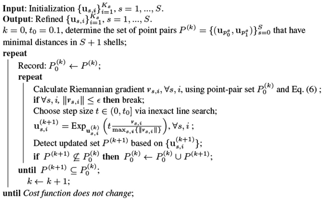One important issue of the proposed Riemannian gradient descent method is that, after each gradient descent, the set of point pairs $\left\{\right({\mathbf{u}}_{p_0^s},{\mathbf{u}}_{p_1^s}\left)\right\}$ with minimal distances may change, and the cost function and its gradient, which depends on these pairs, may also change. To solve this issue, in each iteration, we compare the updated set of point pairs with the previous pair set before the one step gradient descent, and if the updated pair set has some new pairs which are not in the previous pair set, then we re-perform the gradient descent using the joint set of these two sets. See Algorithm 1 for implementation details. The algorithm is efficient and converges in seconds.

Since the optimization problem is highly non-convex, a good initialization is important for a good solution. Initialization can be set as a set of random points, the solution given by incremental estimation, or the solution given by MILP. Note that when using MILP for the initialization, solving the CSC becomes slow when a large number of points are involved. In practice, we apply MILP to 321 points obtained from spherical tessellation and use the MILP solution as the initialization of the gradient descent method for CSC.

3. Experiments

Separation of Sampling Schemes.

We evaluated the effectiveness of the proposed multi-shell MILP-based DSC method in Eq. (4a) with w = 1, by gauging whether it can separate points on a set of samples into several subsets, keeping the points in each subset as uniform as possible. We used the subsetpoints program in CAMINO [1,2] for comparison, which performs the same task by using simulated annealing. For this evaluation, we randomly mixed two sets of uniform points, one set consisting of 81 points generated by spherical tessellation and the other set consisting of 60 points from CAMINO generated by EEM. Separation of these 141 points into subsets respectively with 81 and 60 samples should ideally give results that match the original uniform point sets. Our method, which uses MILP, gave results that exactly match the original point sets within 5 seconds. subsetpoints in CAMINO saves the result every hour when it runs. It gave two incorrect points in each subset after running for 2 hours, 7 incorrect points after 8 hours, and the correct result after 9 hours. Although the correct result had been obtained, the program continued to run for hours until the simulated annealing temperature was finally small enough.

Multi-shell Angular Separation.

We evaluated the effectiveness of the proposed multi-shell DSC (MILP) and CSC (incremental estimation) methods in generating a three shell sampling scheme, each shell consisting of K sampling points. We tested two cases: K = 28 and K = 90. These two cases were used such that we could compare our results with those given by gEEM and incremental gEEM [4]; results for 28 points per shell were reported in [4] and results for 90 points per shell were utilized in the HCP. MILP was used to select K × 3 points from 321 points given by spherical tessellation. In incremental CSC, the selection was carried out using 20481 uniformly distributed points. Gradient descent was then used to refine these results. In Table 1, the covering radii, i.e., the minimal angular differences, of these results were compared with those given by gEEM and incremental gEEM [4]. The multi-shell results of gEEM with K = 28 were extracted from [4]. The results of incremental gEEM with K = 28, 90, which have been used in HCP, were obtained from the website³ created for [4]. The covering radii for single-shell results given by EEM in CAMINO are shown for reference. Fig. 1 visualizes the results with K = 28 generated by incremental gEEM, incremental CSC, and gradient descent with MILP initialization. Table 1 and Fig. 1 demonstrate clearly that the proposed MILP method and incremental CSC estimation yield larger covering radii than gEEM and incremental gEEM in all three shells and the combined shell containing all points. The proposed gradient descent method with MILP initialization yields the best angular separation in the multi-shell case, and its results are comparable with the single-shell results given by EEM in CAMINO, although the optimization was done with respect to all shells.

Table 1.

Covering radii of multi-shell sampling schemes with number of samples 28 × 3 and 90 × 3 generated by various methods. Note that gEEM results for 90 × 3 are not available in [4], and EEM results from CAMINO are individually for each single shell (the scheme with 270 samples is not available).

	Shell 1 (28)	Shell 2 (28)	Shell 3 (28)	Combined (28 × 3)
gEEM [4]	22.2°	22.2°	22.0°	13.2°
Incr. gEEM [4]	19.2°	19.7°	19.3°	4.7°
Incr. CSC (N = 20481)	21.3°	19.3°	21.1°	10.5°
MILP (N = 321)	23.8°	23.8°	24.3°	13.3°
Incr. CSC + Grad. Desc.	24.3°	23.5°	24.2°	10.9°
MILP + Grad. Desc.	25.7°	25.7°	25.4°	13.6°
EEM (CAMINO) [1,2]	25.7°	25.7°	25.7°	15.6°
	Shell 1 (90)	Shell 2 (90)	Shell 3 (90)	Combined (90 × 3)
Incr. gEEM [4]	10.8°	10.3°	10.5°	2.4°
Incr. CSC (N = 20481)	10.4°	9.7°	10.4°	4.6°
MILP (N = 321)	13.3°	13.5°	13.3°	7.9°
Incr. CSC + Grad. Desc.	13.0°	13.5°	12.8°	5.2°
MILP + Grad. Desc.	14.6°	15.0°	14.8°	7.5°
EEM (CAMINO) [1,2]	15.1°	15.1°	15.1°	-

Fig. 1.

Multi-shell sampling schemes with 28 × 3 samples generated by three methods and their combined covering radii showed in Table 1. The colors differentiate the sampling points from the three shells.

Rotational Invariance in Reconstruction.

We tested the multi-shell sampling schemes with 28 × 3 samples in Table 1 on whether they give consistent reconstruction results for the synthetic signals generated by rotated models. A mixture of tensor model was used: E(qu) = 0.5 exp(−q²u^TD₁u) + 0.5 exp(−q²u^TD₂u), where b = q² = 1000, 2000, 3000 s/mm², and the two tensors D₁, D₂ have the same eigenvalues [1.7, 0.2, 0.2] × 10⁻³ mm²/s and have a crossing angle of 60°. This signal generation is repeated 20481 times by rotating the model according to 20481 uniformly distributed directions generated by spherical tessellation. We performed Spherical Polar Fourier Imaging (SPFI) with spherical order 6 and radial order 2 [11] to estimate the EAP profiles with radius of 15μm, detected the peaks of the EAP profiles, and compared the detected peaks with the ground-truth fiber directions in these 20481 tests. The means and standard deviations are shown in Table 2. Note that we have omitted the results for gEEM because the algorithm is not publicly available. It is clear from the table that the proposed methods yield significantly lower mean angular differences (paired t-test, p < 0.001) with lower standard deviations than incremental gEEM. Similar to Table 1, gradient descent with MILP initialization gives the best result.

Table 2.

Angular differences between estimated and ground-truth fiber directions for the sampling schemes generated by different methods

	Incr. CSC	Incr. CSC + Grad. Desc.	MILP	MILP + Grad. Desc.	Incr. gEEM
Angular Difference	1.44° ± 0.69°	1.40° ± 0.69°	1.30° ± 0.68°	1.29° ± 0.68°	1.72° ± 0.79°

4. Conclusion

To our knowledge, this is the first work on designing single-/multi-shell sampling schemes using continuous spherical code (CSC) and discrete spherical code (DSC) formulations. We propose an incremental estimation method for both CSC and DSC, a mixed-integer linear programming (MILP) method for DSC, and a Riemannian gradient descent method for CSC. The experimental results showed that, compared with the gEEM method and its incremental variant that has been used in the HCP, the sampling schemes by the proposed gradient descent with MILP initialization and incremental CSC yield larger covering radius and better rotation invariance.

References

- 1.Jones DK, Horsfield MA, Simmons A: Optimal strategies for measuring diffusion in anisotropic systems by magnetic resonance imaging. Magnetic Resonance in Medicine 42, 515–525 (1999) [PubMed] [Google Scholar]
- 2.Cook P, Bai Y, Nedjati-Gilani S, Seunarine K, Hall M, Parker G, Alexander D: Camino: Open-source diffusion-MRI reconstruction and processing. In: ISMRM (2006) [Google Scholar]
- 3.Caruyer E, Cheng J, Lenglet C, Sapiro G, Jiang T, Deriche R: Optimal Design of Multiple Q-shells experiments for Diffusion MRI. In: CDMRI Workshop, MICCAI 2011 (2011) [Google Scholar]
- 4.Caruyer E, Lenglet C, Sapiro G, Deriche R: Design of multishell sampling schemes with uniform coverage in diffusion MRI. Magnetic Resonance in Medicine (2013) [DOI] [PMC free article] [PubMed] [Google Scholar]
- 5.Sotiropoulos SN, Jbabdi S, Xu J, Andersson JL, Moeller S, Auerbach EJ, Glasser MF, Hernandez M, Sapiro G, Jenkinson M, et al. : Advances in diffusion MRI acquisition and processing in the Human Connectome Project. NeuroImage 80, 125–143 (2013) [DOI] [PMC free article] [PubMed] [Google Scholar]
- 6.Conway JH, Hardin RH, Sloane NJ: Packing lines, planes, etc.: Packings in Grassmannian spaces. Experimental Mathematics 5(2), 139–159 (1996) [Google Scholar]
- 7.Deriche R, Calder J, Descoteaux M: Optimal real-time q-ball imaging using regularized kalman filtering with incremental orientation sets. Medical Image Analysis 13(4), 564–579 (2009) [DOI] [PubMed] [Google Scholar]
- 8.Tóth LF: On the densest packing of spherical caps. The American Mathematical Monthly 56(5), 330–331 (1949) [Google Scholar]
- 9.Gurobi Optimization, Inc.: Gurobi optimizer reference manual (2014) [Google Scholar]
- 10.Cheng J, Ghosh A, Jiang T, Deriche R: A Riemannian Framework for Orientation Distribution Function Computing. In: Yang G-Z, Hawkes D, Rueckert D, Noble A, Taylor C (eds.) MICCAI 2009, Part I. LNCS, vol. 5761, pp. 911–918. Springer, Heidelberg: (2009) [DOI] [PubMed] [Google Scholar]
- 11.Cheng J, Ghosh A, Jiang T, Deriche R: Model-free and Analytical EAP Reconstruction via Spherical Polar Fourier Diffusion MRI. In: Jiang T, Navab N, Pluim JPW, Viergever MA (eds.) MICCAI 2010, Part I. LNCS, vol. 6361, pp. 590–597. Springer, Heidelberg: (2010) [DOI] [PubMed] [Google Scholar]