Effect of Ventilation Velocity on Hexavalent Chromium and Isocyanate Exposures in Aircraft Paint Spraying

Abstract

Exposure control system performance was evaluated during aircraft paint spraying at a military facility. Computational fluid dynamics (CFD) modeling, tracer gas testing, and exposure monitoring examined contaminant exposure versus crossflow ventilation velocity. CFD modeling using the RNG k-ε turbulence model showed exposures to simulated methyl isobutyl ketone of 294 and 83.6 ppm, as a spatial average of five worker locations, for velocities of 0.508 and 0.381 m/s (100 and 75 fpm) respectively. In tracer gas experiments, observed supply/exhaust velocities of 0.706/0.503 m/s (136/99 fpm) were termed full-flow, and reduced velocities were termed 3/4-flow and half-flow. Half-flow showed higher tracer gas concentrations than 3/4-flow, which had the lowest time-averaged concentration, with difference in log means significant at the 95% confidence level. Half-flow compared to full-flow and 3/4-flow compared to full-flow showed no statistically significant difference. CFD modeling using these ventilation conditions agreed closely with the tracer results for the full-flow and 3/4-flow comparison, yet not for the 3/4-flow and half-flow comparison. Full-flow conditions at the painting facility produced a velocity of 0.528 m/s (104 fpm) midway between supply and exhaust locations, with the supply rate of 94.4 m3/s (200,000 cfm) exceeding the exhaust rate of 68.7 m3/s (146,000 cfm). Ventilation modifications to correct this imbalance created a mid-hangar velocity of 0.406 m/s (80.0 fpm). Personal exposure monitoring for two worker groups—sprayers and sprayer helpers (“hosemen”)—compared process duration means for the two velocities. Hexavalent chromium (Cr[VI]) exposures were 500 vs. 360 μg/m3 for sprayers and 120 vs. 170 μg/m3 for hosemen, for 0.528 m/s (104 fpm) and 0.406 m/s (80.0 fpm) respectively. Hexamethylene diisocyanate (HDI) monomer means were 32.2 vs. 13.3 μg/m3 for sprayers and 3.99 vs. 8.42 μg/m3 for hosemen. Crossflow velocities affected exposures inconsistently, and local work zone velocities were much lower. Aircraft painting contaminant control is accomplished better with the unidirectional crossflow ventilation presented here than with other observed configurations. Exposure limit exceedances for this ideal condition reinforce continued use of personal protective equipment.

INTRODUCTION

National Institute for Occupational Safety and Health (NIOSH) researchers investigated ventilation system performance in military aircraft paint finishing hangars as a function of air velocity delivered by the system to the work area. Previous investigations at the subject facility found exposures to isocyanates and hexavalent chromium exceeded occupational exposure limits (OELs).⁽¹⁾ Isocyanates are respiratory sensitizers and have health effects in both monomeric and oligomeric forms.^(2,3,4,5) Hexavalent chromium exposure can cause nasal irritation and damage, and respiratory cancer, among other conditions.⁽⁶⁾

OSHA standard, 29 CFR 1910.94 – Ventilation, requires that spray booths maintain an air velocity in the booth cross-section of 100 fpm (0.508 m/s).⁽⁷⁾ However, an OSHA interpretation of 1910.94 prepared for the subject facility stated that its hangar is a spray area rather than a booth. Evaluating ventilation performance, then, should perhaps focus more on exposure control than velocity achievement, although 100 fpm (0.508 m/s) is still required by the 2010 Uniform Facilities Criteria (UFC).⁽⁸⁾ The hexavalent chromium (Cr[VI]) standard, 29 CFR 1910.1026, part (f)(1)(ii), on painting large aircraft, allows respiratory protection to achieve the PEL (5 μg/m³), if 8-hr TWA concentrations controlled through other methods do not exceed 25 μg Cr[VI]/m³, “unless the employer can demonstrate that such controls are not feasible.”⁽⁹⁾ Interestingly, the ACGIH recommends only 50 fpm (0.254 m/s) for large vehicle paint booths.⁽¹⁰⁾

The subject facility was designed to meet the 100 fpm (0.508 m/s) velocity specification; however, separate bays of the facility consistently operated at velocities that differed from the specification. The bays were geometrically identical, including the ventilation configuration, and the air handling equipment for each bay was of the same brand and model number. Operational differences were attributed to controller settings, wear, and filter loading. These facts allowed investigation of velocity as an exposure determinant.

Motivation for the investigation came from exceedances of OELs when the ventilation system met the OSHA and UFC criterion of 5.08 m/s (100 fpm). A question followed naturally—is this velocity the most protective? Understanding the effect of velocity (within a reasonable range) on exposure then became the study focus, with the large effect of velocity on energy use a secondary consideration.

Four supply and four exhaust fans served each bay, with exhaust rpm linked to supply function via variable frequency drive (VFD) controllers. Two supply fans were equipped with steam heat elements. In this crossflow ventilation design, air enters through a supply wall filter bank; the flow expands slightly into the hangar cross section, which contains the aircraft, and then accelerates into an exhaust filter bank that covers a substantial area of the wall at the opposite end. Performance is sensitive to exhaust filter loading, and the current replacement criterion is a pressure drop of 2.5 in. water gauge across the filter bank. Crossflow ventilation, the intentional application of airflow through a space, from a supply location to an exhaust location, should not be confused with cross drafts, which are generally undesired flows sideways to the designed flow direction.

METHODS

Ventilation Evaluation

Velocities were measured using an ADM-860 AirData Multimeter (Shortridge Instruments, Inc., Scottsdale AZ), a Shortridge VelGrid, two sections of 20-foot Tygon^® tubing, and a 25-foot extension pole. Pressure drop across the exhaust filter bank was read from the control room manometer before each painting phase to verify proper operation. In addition, differential pressures were measured across bay/ambient, bay/control room, and control room/ambient boundaries, using the ADM-860 Multimeter. During the initial and follow-up field surveys, velocity measurements were taken in a matrix of 16 locations in a plane midway between the supply and exhaust. Ventilation system modifications involved installation of new variable frequency drive (VFD) controllers to balance the flow.

The supply and exhaust filter banks in these bays were smaller than the cross-sectional area of the hangar. All air velocities (V_CS) reported here were normalized to the area of the hangar cross-section (A_CS), using the formula

$$V_{CS}=\frac{A}{A_{CS}}V,$$ Eqn. 1

where A and V are the face area and face velocity of the supply or exhaust filter banks. This approach was used to facilitate comparison with regulations and guidance for spray operations ventilation, which are given as velocities in the occupied cross-section, rather than as volumetric flow rates. The supply and exhaust filter areas were 86.6% and 37.5% of the cross-sectional area, respectively (Figure 1).

Figure 1.

Drawing of the aircraft painting bay showing filter areas.

Air Sampling

Comprehensive air sampling evaluating concentrations of compounds in paints, primers, and solvents used on F/A-18C/D Hornet strike fighter aircraft was reported previously.⁽¹⁾ The current study includes follow-up sampling of total particulate matter (TPM), hexavalent chromium Cr[VI], and hexamethylene diisocyanate (HDI) after ventilation system modifications. Although sampling was performed during painting of C-2 and E-2 aircraft in the follow-up survey, these processes were not sampled in the original work. Thus, two velocities—before and after ventilation modifications—were tested only for the F-18 aircraft.

TPM and Cr[VI] air samples were collected on pre-weighed polyvinyl chloride (PVC) filters at a flow rate of 2.0 liters per minute (lpm) and analyzed according to NIOSH Methods 0500 and 7605 respectively.^(11,12) HDI was collected on glass fiber filters impregnated with 1-(9-anthracenylmethyl)piperazine (MAP) at a flow rate of 1.0 lpm. After sampling, the filters were field-extracted in 5 ml solutions of acetonitrile with 1 × 10⁻⁴ M MAP. Analyses followed NIOSH Method 5525.⁽¹³⁾ Oligomeric HDI is presented in terms of isocyanate functional group (NCO) mass, and HDI monomer is presented as monomer mass. The HDI filter samples were analyzed by the Chemical Exposure & Monitoring Branch of NIOSH (Cincinnati, OH). Bureau Veritas North America (Novi, MI) performed all other analyses. Both laboratories are accredited by the American Industrial Hygiene Association (AIHA).

Sampling was performed during the specific painting phases rather than over the entire work shift because Cr[VI] and HDI exposures occurred only in one phase, e.g. Cr[VI] during priming (Figure 2). Sampling began (ended) as the artisans put on (took off) their required PPE and thus included material handling and tool clean-up. Break or lunch occurred between phases, in a separate building.

FIGURE 2.

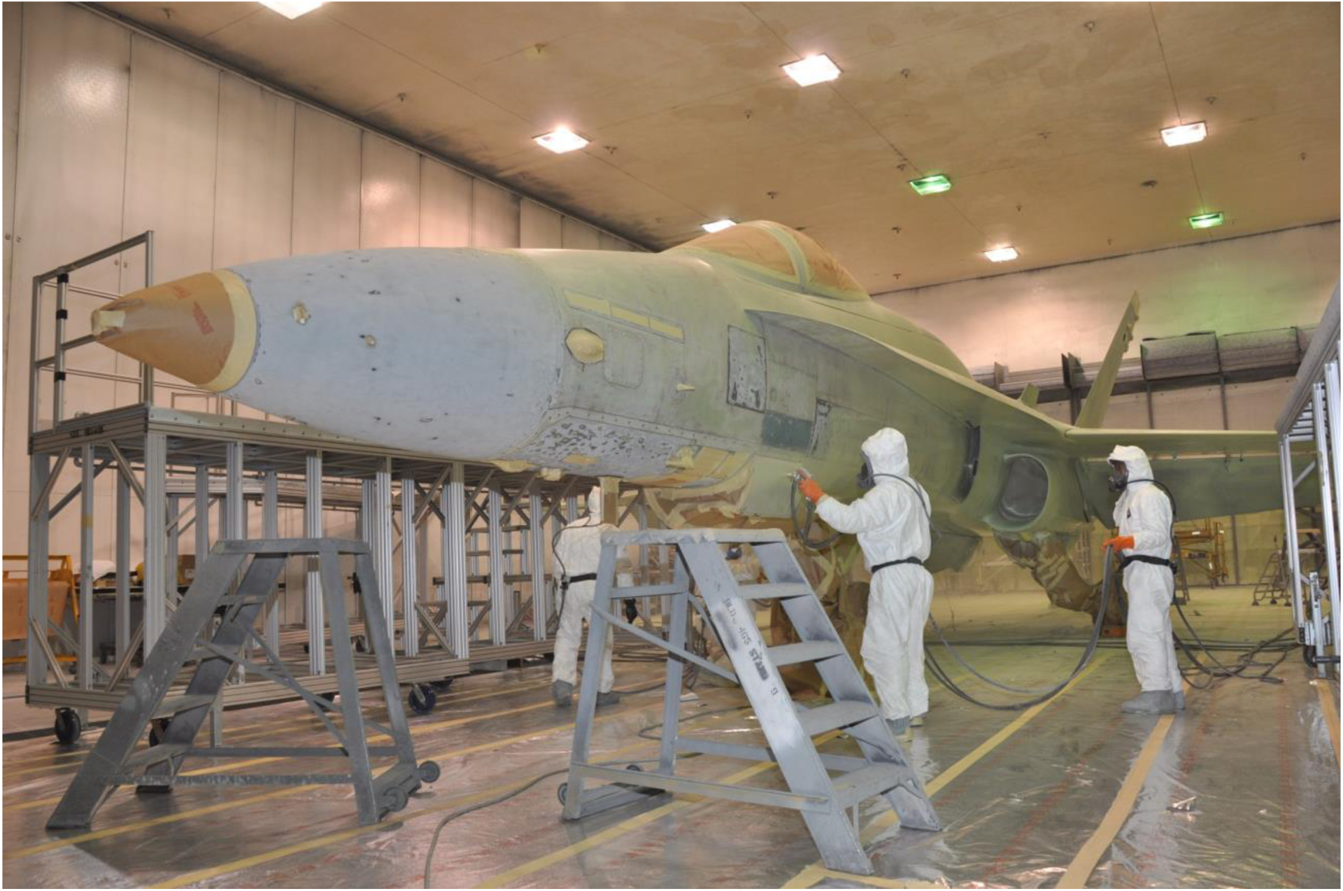
Navy artisans (sprayers and hosemen) applying primer during F-18 strike fighter aircraft paint finishing operations.

Statistical Comparisons

The statistical power to discern exposures differences was increased by combining the exposure data from all four contaminants measured, while grouping according to job classification to reduce variance. For each contaminant, the exposures were normalized by comparing the six observations from the original survey to the single observation in the follow-up survey. This single observation was treated as a reference value, and a percent-difference was calculated, forming N = 6 × 4 = 24 comparisons by velocity. Statistical analysis showed that the personal exposure data were log-normally distributed, and a t-test was performed on the log-transformed data. This process was followed separately for hosemen and for sprayers. It can be argued that repeatedly using the reference concentration overweights a single data point. Thus, a t-test was also performed comparing the eight means for sprayers and hosemen (combined) from the original survey, to the eight single follow-up observations.

CFD Methods

CFD is a numerical method that solves the system of equations that describe fluid flow by simulating real process geometry and sources within a spatial computational grid. In the CFD simulationss presented here, the steady-state, differential form of the incompressible Navier-Stokes equations, along with the transport equations for turbulence quantities and species mass, were discretized to the computational grid, using the SIMPLE algorithm and the second-order upwind discretization scheme. Simulations were performed for a variety of ventilation settings representing both balanced and unbalanced flow rates. Aircraft surfaces and hangar wall, floor, and ceiling were modeled as no-slip walls, except that for the unbalanced flow conditions, the ceiling was modeled as a zero-gauge pressure boundary.

The ventilation boundary conditions are listed in Table I, along with other model inputs. The basis for these inputs was ventilation design targets, real conditions measured during operation, and in the case of the spray gun, manufacturer’s specifications. Some assumptions were made, including the turbulence intensity (TI) and characteristic length scale (L) for the supply, exhaust, and spray airflows. It was assumed that TI was 10%, and L was 1 m for the filter boundary conditions and 0.1 m for the spray. L was estimated from the approximately 1 m spacing of the iron framework that supported the filter banks and the approximately 0.1 m spraying opening at the end of the modeled worker arm. The 10% TI assumption was tested by running the 0.508 m/s (100 fpm) simulation again, using a TI of 5% at the filter boundaries. Contour plots of TI in the hangar centerplane were indistinguishable for these two conditions. Tu has written that a TI of between 5% and 10% is appropriate for internal airflows.⁽¹⁴⁾ Another assumption was that the velocity profiles of the supply and exhaust filter faces were uniform, while in reality there was a range of velocities measured across the filters. While this decision simplified the modeling effort, it was also meant to represent the intended function of the plenum filter design.

TABLE I.

Implementation of painting facility parameters in CFD simulations

Bay Velocity m/s (fpm)	Interior Surface	Boundary Type	Velocity m/s	Contaminant mass fraction	Turbulence intensity	Turbulence length-scale	Turbulence Model
0.549 (108)	SUPPLY FILTER	VELOCITY INLET	0.6338	zero	10%	1 m	Standard k- ε
	EXHAUST FILTER	VELOCITY INLET	−1.465	Not specified	Not specified	Not specified
	SPRAYER HAND	VELOCITY INLET	1.71	0.5	10%	0.1 m
0.440 (86.6)	SUPPLY FILTER	VELOCITY INLET	0.4754	zero	10%	1 m	Standard k- ε
	EXHAUST FILTER	VELOCITY INLET	−1.174	Not specified	Not specified	Not specified
	SPRAYER HAND	VELOCITY INLET	1.71	0.5	10%	0.1 (m)
0.330 (65.0)	SUPPLY FILTER	VELOCITY INLET	0.381	zero	10%	1 m	Standard k- ε
	EXHAUST FILTER	VELOCITY INLET	−0.8816	Not specified	Not specified	Not specified
	SPRAYER HAND	VELOCITY INLET	1.71	0.5	10%	0.1 m
0.220 (43.3)	SUPPLY FILTER	VELOCITY INLET	0.2540		10%	1 m	Standard k- ε
	EXHAUST FILTER	VELOCITY INLET	−0.5877	Not specified	Not specified	Not specified
	SPRAYER HAND	VELOCITY INLET	1.71	0.5	10%	0.1 (m)
0.549/0.330 (108/65.0)	SUPPLY FILTER	VELOCITY INLET	0.6338	zero	10%	1 m	Standard k- ε
	EXHAUST FILTER	VELOCITY INLET	−0.8816	Not specified	Not specified	Not specified
	SPRAYER HAND	VELOCITY INLET	1.71	0.5	10%	0.1 (m)
0.508 (100)	SUPPLY FILTER	VELOCITY INLET	0.5865	zero	10%	1 m	RNG k-ε
	EXHAUST FILTER	VELOCITY INLET	−1.3563	Not specified	Not specified	Not specified
	SPRAYER HAND	VELOCITY INLET	1.71	0.5	10%	0.1 m
0.381 (75)	SUPPLY FILTER	VELOCITY INLET	0.4399	zero	10%	1 m	RNG k- ε
	EXHAUST FILTER	VELOCITY INLET	−1.017	Not specified	Not specified	Not specified
	SPRAYER HAND	VELOCITY INLET	1.71	0.5	10%	0.1 m
0.254 (50)	SUPPLY FILTER	VELOCITY INLET	0.2933	zero	10%	1 m	RNG k- ε
	EXHAUST FILTER	VELOCITY INLET	−0.6782	Not specified	Not specified	Not specified
	SPRAYER HAND	VELOCITY INLET	1.71	0.5	10%	0.1 m

Notes: The grid of 9,476,802 cells was adapted to a fine grid of 16,241,731 cells (a 42% increase) to test grid independence. Spray nozzle velocity was taken from the manufacturer’s specification of 11 cfm: V = Q/A = 11 cfm/0.00304 m². Aircraft surfaces and hangar wall, floor, and ceiling were modeled as no-slip walls, except that for the unbalanced flow condition, the ceiling was modeled as a zero-gauge pressure boundary.

A user-defined contaminant that was given the physical properties (e.g. density and viscosity) of methyl isobutyl ketone (MIBK) was emitted at a volumetric flow rate specified by the spray gun manufacturer, in vapor form, from the hand areas of two simulated workers placed at commonly observed spraying locations. The launch velocity boundary condition was determined by the ratio of the flow rate to the face area of the mesh cell at the center of the sprayer’s arm end, without attempting to match the velocity distribution emitted from the actual spray gun nozzle (Table I). The modeled MIBK vapor density was 4.23 kg/m³, about 3.5 times denser than air, and its viscosity was 6.70 × 10⁻⁶ kg/m-s, less than half that of air. Once dispersed, the fluid properties were determined by the volume fractions of contaminant and clean air in the hangar air mixture, according to the species concentration determined by the coupled solution process, wherein flow, turbulence, and concentration variables are updated in each iteration.

Although the workers in the real process sprayed with a side-to-side or up-and-down arm motion and stopped spraying while they moved to a different section of the airframe, the steady-state simulations treated the source as continuous and static. The rationale for simplifying the painting process into a single time slice was that the modeling goal of comparing exposures at different velocities was fulfilled. Static sources at a single set of observed positions is a loss in the fidelity of absolute exposure estimation; however, estimation of exposure differences due to different velocities is reasonable by this method. This limitation of the simulations makes clear the importance of real process exposure monitoring, for determination of absolute rather than relative exposures.

A 9.5 million cell unstructured mesh, composed of both tetrahedral and hexahedral elements, of an F/A-18C/D Hornet in the hangar space was generated using Gridgen software (Pointwise, Inc., Fort Worth TX). The extent of the computational domain matched the interior of the hangar bay depicted in Figures 1, 2 and 3. The modeled geometry included positions of wing flaps, elevators, and rudders, observed during painting (Figures 2 and 3). Hosemen (H) were placed farther from the aircraft and downwind from their sprayer (S) partners. The contaminant source was located at the end of the sprayers’ right arms. One sprayer was on a scaffold. Solid models representing workers in Tyvek^® suits (Figure 4) were developed in Solidworks (Dassault Systemes SolidWorks Corp., Concord MA). The mesh was imported into Fluent 6.3 (ANSYS, Inc., Canonsburg PA).

FIGURE 3.

Geometry of workers, exhaust wall filter, and F/A-18C/D Aircraft.

FIGURE 4.

Detail of modeled worker geometry.

Turbulence was modeled using the Reynolds-averaged Navier–Stokes (RANS) k-ε model. In the earlier exploratory simulations, the standard k-ε model was used, because it tends to provide a stable solution process. In later simulations, which sought greater accuracy, a form of the k-ε model that incorporates renormalization group theory (RNG)⁽¹⁵⁾ was used. Iterative instability in the steady-state solution was addressed by setting the under-relaxation parameters for pressure correction, velocity, and turbulence very low. The pressure parameter was kept highest, at 0.4, while the velocity components and the turbulence kinetic energy (TKE) were reduced to 0.3. Convergence difficulty, or “stiffness,” in the eddy dissipation rate equation that is typical of indoor airflow CFD simulations was handled by setting its underrelaxation parameter to 0.2. No underrelaxation was applied to the density or passive scalar (MIBK) concentration equations.

The solutions were first initialized by applying the supply filter boundary conditions—velocity, TI (10%), L (1 m), and MIBK concentration (zero)—to all fluid cells in the domain. Then, the solutions were brought to iterative convergence, where the normalized residuals (measures of relative error in the equations that govern fluid motion) were all less than 10⁻³, using the first order upwind discretization scheme.⁽¹⁶⁾ This process required fewer than 1,000 iterations in all cases. All simulations were then run for 38,000 iterations, using second order upwind discretization, where the normalized residuals were below 10⁻⁴, except in the case of species (less than10⁻⁵) and eddy dissipation rate (slightly greater than 10⁻⁴). The species concentration never reached a clearly asymptotic steady-state but was observed to achieve stationarity—regular fluctuations within a consistent, limited range. The fixed and large number of iterations was used as the ultimate convergence requirement to ensure that exposure comparisons among flow conditions were free of convergence errors, or that at least the convergence error was very small and similar for all flow conditions, which would still allow a reasonably accurate comparison.

Verification and Validation

Verification consisted of grid indepence trials and examination of first-cell y⁺-values. The original grid of 9,476,802 cells was adapted to a finer grid of 16,241,731 cells (a 42% increase), by halving the linear cell dimensions in the sprayer and hosemen zones, thereby increasing the number of cells in these important areas by a factor of eight. Validation involved comparison of CFD and tracer results, using concentrations averaged across worker locations in the simulations and monitor intake locations in the experiments. In the third set of CFD simulations, imbalanced flow rates were modeled, even though these conditions are not design goals. The imbalanced conditions observed during painting operations and tracer experiments were simulated to compare concentrations predicted by CFD to those measured during the tracer experiments, as validation. Using the notation [supply velocity]/[exhaust velocity], the model boundary conditions for full-flow were 0.706/0.503 m/s (139/99.0 fpm); for 3/4-flow were 0.518/0.350 m/s (102/68.9 fpm); and, for half-flow were 0.371/0.249 m/s (73.4/49.0 fpm). These conditions are shown in Table I.

Initial Investigation of a Range of Crossflow Velocities and Over-supply Imbalance

Balanced rates, as normalized velocities, of 0.220, 0.330, 0.381, 0.440, 0.508, and 0.549 m/s (43.3, 65, 75, 86.6, 100, and 108 fpm) were modeled, along with an unbalanced rate of 0.549/0.330 m/s (108/65 fpm), supply/exhaust. The unbalanced rate represented observed conditions and exploratory stationary operating states that would be created by turning off certain fans in the existing system.For these exploratory simulations, the standard k-ε model was employed. The velocity boundary conditions are shown in Table I.

Comparison of 0.508 m/s (100 fpm) and 0.381 m/s (75 fpm) Crossflow Velocities

For these simulations, balanced airflows in the hangar cross section corresponding to 0.508 m/s (100 fpm) and 0.381 m/s (75 fpm) were modeled. Although these crossflow velocities did not correspond exactly to what was observed during operation, they are important in regulation and design specification. OSHA lists 100 fpm as the required “design” velocity in paint spray booths and spray rooms, with 75 – 125 fpm given as the “range.” ⁽⁷⁾ For these simulations, the RNG k-ε turbulence model was used. These conditions are given in Table I.

Tracer Experiments

Sulfur hexafluoride (SF₆) was released in the unoccupied hangar—with the F-18 aircraft in place—at the normal supply/exhaust flow rate and at lower flow rates, and concentrations were measured at various locations. The concentrations of SF₆ were compared among three unbalanced flow rates—half, 3/4, and full capacity determined by the number of supply blowers operating—with the exhaust attempting to match these rates and falling short, in each case. Thus, the experiments were conducted with this system operating normally, and with one of four supply-exhaust pairs powered down and also with two supply-exhaust pairs down. SF₆ was released continuously at the aircraft nose and measured at five observed worker locations, using MIRAN SapphIRe portable real-time infrared monitors (Thermo Fisher Scientific Co., Waltham MA).

In addition to the comparison with CFD results described previously, the tracer experiments were used to evaluate the effect of ventilation velocity on exposure. Several 15-minute trials were run, in a randomized factorial design, with “ventilation setting” as the independent variable and time-averaged SF₆ concentration the dependent variable.⁽¹⁷⁾ A multiple comparison analysis was performed using Tukey’s studentized range test.on the log mean concentrations, with velocity scenario as a categorical variable, with three values. Significance was evaluated at the 95%-confidence level.

RESULTS

Air Velocities

In the initial survey, the supply rate of 94.4 m³/s (200,000 cfm) produced an average velocity of 0.798 m/s (157 fpm) at the supply filter face. The supply velocity normalized to the hangar cross-section was 0.691 m/s (136 fpm), which exceeded the original design specification of 0.508 m/s (100 fpm). The exhaust rate of 68.7 m³/s (146,000 cfm) produced an average velocity of 1.34 m/s (264 fpm) at the exhaust filter face, which normalized to 0.504 m/s (99.3 fpm). As shown in Table III, these supply and exhaust conditions created a measured velocity of 0.528 m/s (104 fpm) in the mid-hangar work zone. In the follow-up survey, the average mid-hangar velocities were 0.412 m/s (81.1 fpm) for the large bay created by combining Bays 7 and 8 and 0.406 m/s (80.0 fpm) for Bay 2.

TABLE III.

Process information, ventilation measurements, and process duration TWAs

Measurement Location or Job Class	What was Measured (units)	F-18 Painting Bay 6 (Initial Survey)	N	E-2 Painting Bays 7–8 (Post-mod)	N	C-2 Painting Bays 7–8 (Post-mod)	N	F-18 Painting Bay 2 (Post-mod)	N
Mid-Hangar	Mean Velocity, m/s (fpm)	0.528 (104)	20	0.412 (81.1)	8	0.412 (81.1)	8	0.406 (80.0)	8
	Paint Quantity (gal)	13	1	16	1	18	1	13	1
	Paint Formula HDI monomer/HDI oligomer (% NCO)	0.143/9.97	1	0.022/4.53	1	0.016/5.16	1	0.043/9.27	1
Sprayer mean/gmean [range]	HDI monomer (μg/m3)	33.1/32.2 [25.0, 49.6]	6	11.3/10.5 [6.06, 14.2]	3	7.31/7.25 [6.37, 8.26]	2	30.9	1
	HDI oligomer (μg NCO/m3)	279/259 [178, 484]	6	191/169 [78.6, 265]	3	242/242 [240, 245]	2	725	1
	TPM (mg/m3)	20/18 [7.0, 26]	6					14	1
	Cr[VI] (μg/m3)	530/500 [220, 650]	6					360	1
Hoseman mean/gmean [range]	HDI monomer (μg/m3)	6.19/3.99 [<0.7, 11.3]	6	3.88/3.62 [2.49, 5.27]	2			19.6	1
	HDI oligomer (μg NCO/m3)	81.7/42.7 [<3, 153]	6	61.5/54.9 [33.8, 89.2]	2			673	1
	TPM (mg/m3)	5.2/4.3 [1.4, 10]	6					5.9	1
	Cr[VI] (μg/m3)	150/120 [37, 300]	6					170	1

Note: Values below the LOQ (indicated by the < symbol) were divided by √2 for calculation of means.

Air Sampling

Table III provides exposure data for paint finishing operations on three aircraft and two airflow velocities, before and after ventilation modifications, although the matrix is not complete. For the sprayer job class, mean exposures measured at the lower velocity were below the single exposures measured at the higher velocity, for HDI monomer, TPM, and Cr[VI}, yet were above the higher velocity exposure for HDI oligomer. For the hoseman job class, mean exposures measured at the lower velocity were above the single exposures measured at the higher velocity for all four contaminants.

Aircraft Primer Paint Spraying

TPM process duration TWAs for sprayers in the current survey was 14 mg/m³ compared to 18 mg/m³ in the initial survey, and TPM for hosemen in the current survey was 5.9 mg/m³ compared to 4.3 mg/m³ in the initial survey. The single-measurements, for sprayers and hosemen in the current survey, fell within the initial survey data range, for each job classification.

The Cr[VI] result for sprayers in the current survey was 360 μg/m³ compared to 500 μg/m³ in the initial surveys. The Cr[VI] result for hosemen in the current survey was 170 μg/m³ compared to 120 μg/m³ in the initial survey. The single-value at the lower velocity of the current survey, when compared to the initial survey, was lower for sprayers and higher for hosemen, while remaining within the data range for each job classification.

Aircraft Topcoat Painting

HDI monomer geometric means, comparing results for all three aircraft in the follow-up survey to the initial survey (F-18 only), were 13.3 μg/m³ vs. 32.2 μg/m³ for sprayers and 8.42 μg/m³ vs. 3.99 μg/m³ for hosemen, while oligomer concentrations (as NCO) were 310 μg/m³ vs. 259 μg/m³ for sprayers and 192 μg/m³ vs. 42.7 μg/m³ for hosemen. Although the work task of painting C-2, E-2, or F-18 aircraft was observed to be essentially the same, differences in coating composition and aircraft geometry introduce some variability. Looking only within the F-18 data, then, HDI monomer results were 30.9 μg/m³ vs. 32.2 μg/m³ for sprayers and 19.6 μg/m³ vs. 3.99 μg/m³ for hosemen, while oligomer concentrations (as NCO) were 725 μg/m³ vs. 259 μg/m³ for sprayers and 673 μg/m³ vs. 42.7 μg/m³ for hosemen.

Statistical Comparisons

Table IV compares exposures according to bay ventilation velocity. Bay velocity had a statistically significant effect for hosemen, and the negative mean difference (Table V) indicates that lower velocity led to higher exposure. This result is consistent with the dynamic dilution concept, and conservation of mass requires that within some zone in the ventilated space, higher velocity will create lower concentration. The effect was not seen for sprayers, where the mean difference comparing higher velocity exposures to lower velocity exposures was positive, while not statistically significant. It is possible that the lower velocity was weakly protective for sprayers, but a reasonable interpretation is that it had no discernable effect. When the t-test was done on the mean differences with hosemen and sprayers combined (N reduced to 8), significance disappeared, as the 95% confidence interval included zero.

TABLE IV.

Lognormal t-test on percent differences in exposure for 0.528 m/s (104 fpm) vs. 0.406 m/s (80.0 fpm)

Job Class	N	Mean	Std Dev	Std Err	Minimum	Maximum	95% CL	95% CL	t Value	Pr > |t|
Hosemen	24	−33.69	41.19	8.408	−155.6	29.94	−51.08	−16.29	−4.01	0.0006*
Sprayers	24	0.4488	14.39	2.938	−26.12	23.64	−5.629	6.526	0.15	0.8799
All (means)	8	−16.62	26.69	9.437	−68.40	10.09	−38.93	5.697	−1.76	0.1216

Note: Significance at the 0.05 level is indicated by *.

TABLE V.

Tukey’s studentized range (HSD) test for tracer gas log mean concentration. Means were formed from the five measurement locations

Velocity Comparison	Difference Between Tracer Gas Log Means	Simultaneous 95% Confidence Limits
Half-flow vs. full-flow 0.373/0.249 vs. 0.691/0.503 m/s (73.4/49.0 vs. 136/99.0 fpm)	1.364	−0.2762	3.005
Half-flow vs. 3/4-flow 0.373/0.249 vs. 0.549/0.350 m/s (73.4/49.0 vs. 108/68.9 fpm)	1.961	0.1350	3.787*
3/4-flow vs. full-flow 0.549/0.350 vs. 0.691/0.503 m/s (108/68.9 vs. 136/99.0 fpm)	−0.5968	−2.391	1.197

Note: Comparisons significant at the 0.05 level are indicated by *.

It is worth considering autocorrelation of the samples. HDI monomer and oligomer were collected on one filter, and TPM and Cr[VI] were also collected on one filter. In addition to the NIOSH Method 5525 results reported here, HDI samples were analyzed using OSHA Method 42 and ASSET EZ4-NCO dry-sampler tubes, and the results varied much more widely for the oligomer than for the monomer. Similarly, the Cr[VI] results varied by analysis method (OSHA Method 215 vs. NIOSH Method 7605), while the gravimetric TPM results did not. These facts suggest independence in the samples, because of randomness in the relationship of reported analytes collected on the same filter. The HDI results are clearly independent from the TPM/Cr[VI] results because they were collected on different workers during different painting processes (top-coat vs. primer application). However, if the number of independent observations were reduced because of autocorrelation, the statistical conclusions would move farther away from significance, toward exposures at 104 and 80.0 fpm being indistinguishable.

CFD Modeling

Figure 5 shows concentration contours in the vertical plane bisecting the bay. The shapes of the plumes from the two sprayers (on the scaffold and under the wing) indicate that the crossflow ventilation system provided reasonably directional flow through the work zone, even with the spray momentum and eddy diffusion creating the circular pattern near the sprayers. Figure 6 continues the examination of this centerplane slice to show effects of supply and exhaust boundary condition assumptions. Contours of velocity in Figure 6A show that enforcing conservation of mass by matching the exhaust flow to the supply and spray flows did not interfere with the development of a locally complex and responsive velocity field through the work space. By inspection, floor, ceiling, and aircraft geometry greatly determined the flow, and the exhaust boundary being downstream of the work area limited the effect of assuming filter face velocity uniformity. Figure 6B shows how TI, even moreso than velocity, depends on local flow features. TI of 10% specified at the supply drops to approximately 3% immediately in the domain, consistent with the nature of turbulence to dissipate unless maintained by velocity sheer. In Figure 6C, the mass balance residual being very close to zero throughout the domain indicates that enforcing mass balance by specifying velocities at all domain openings did not prevent solution convergence.

Figure 5.

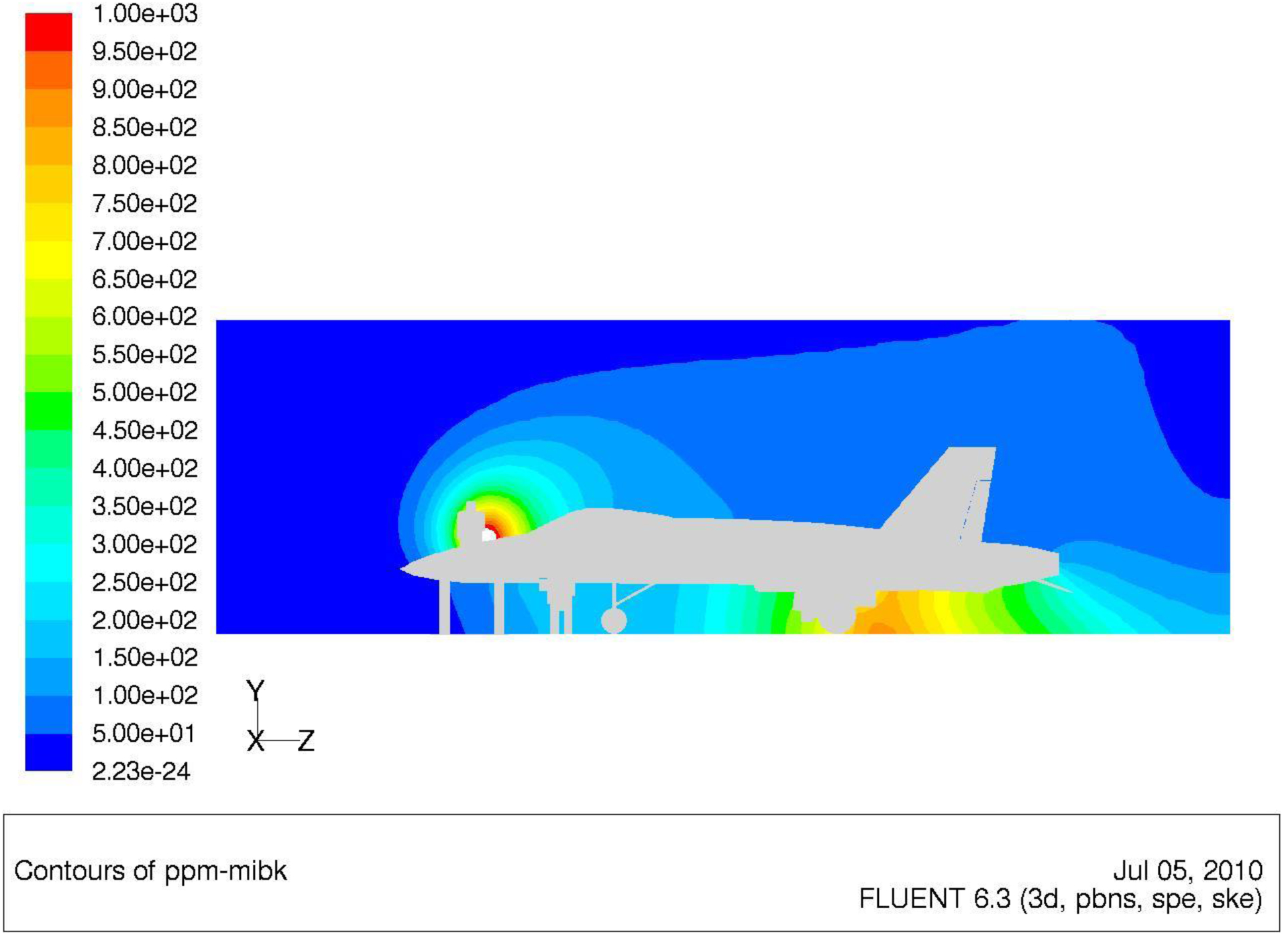
Modeled MIBK concentration contours (ppm) along the centerplane of the painting bay. Seen are the sprayer on the scaffold, the hoseman standing on the ground, and the plume created by the sprayer underneath the far wing.

Figure 6.

Solution contours in the hangar centerplane; (A) Velocity, showing a complex field influenced by ceiling, floor, and aircraft; (B) TI, being mainly determined by internal flow conditions; (C) Mass imbalance residual, where nearly all values are within the interval [−2.44 × 10⁻⁸, 4.70 × 10⁻⁸], i.e. very close to zero.

Figures 7 and 8 show the concentrations at worker locations and means across locations. Figure 7 shows the two least effective rates as 0.220 m/s (43.3 fpm) and the unbalanced 0.549 m/s (108 fpm) supply – 0.330 m/s (65.0 fpm) exhaust scenario based on overall location mean concentrations. These rank first and second highest at four out of five specific worker locations, for the means of worker locations, and for the spatial average at standing breathing zone (BZ height) everywhere in the hangar.

FIGURE 7.

Concentrations of a simulated gas with the properties of MIBK calculated using CFD, for various air velocities and observed worker locations. 0.549/0.330 m/s (108/65 fpm) indicates the unbalanced condition of 0.549 m/s (108 fpm) of supply and 0.330 m/s (65 fpm) of exhaust. “BZ Height” refers to the entire hangar, at a height of 1.50 m from the floor. The heights of “Under Plane,” “Hoseman Port,” “Hoseman Starboard,” “Sprayer Port (scaffold),” and “Sprayer Starboard (wing),” were 0.305 m, 1.50 m, 1.50 m, 3.00 m, and 1.50 m, repectively.

FIGURE 8.

CFD results at 0.381 m/s (75 fpm) and 0.508 m/s (100 fpm) using the RNG k-epsilon turbulence model and a convergence criterion of 10⁻⁴ for the normalized residuals. The lower flow rate yields greater protection on average. “BZ Height” refers to the entire hangar, at a height of 1.50 m from the floor. The heights of “Under Plane,” “Hoseman Port,” “Hoseman Starboard,” “Sprayer Port (scaffold),” and “Sprayer Starboard (wing),” were 0.305 m, 1.50 m, 1.50 m, 3.00 m, and 1.50 m, repectively.

Figure 7 also shows the similarity of 0.330 m/s (65.0 fpm) and 0.440 m/s (86.6 fpm), especially in the difficult to ventilate area under the landing gear hatch, with concentrations of 402 and 401 ppm, respectively. The lowest concentrations occurred for the balanced 0.549 m/s (108 fpm) rate, for all locations other than portside hoseman, which had the lowest concentration at the 0.549/0.330 m/s (108/65.0 fpm) supply/exhaust condition. Additional CFD simulations at 0.381 m/s (75 fpm) produced lower concentrations than 0.508 m/s (100 fpm), at the highest concentration locations. Recall from the Methods section that these simulations used a more accurate turbulence model, and they are reported separately (Figure 8) so that results partly dependent on turbulence model are not attributed to velocity, e.g. 75 vs. 108 fpm (0.381 vs. 0.549 m/s). Concentrations in Figure 8 are generally lower than those in Figure 7, and this effect is due probably to the RNG k-ε model being less isotropically diffusive than the standard k-ε model used in the initial simulations (Figure 7). Figure 8 includes the arithmetic mean because the geometric mean was possibly overly influenced by concentrations being very close to zero at some locations.

Data plotted in Figure 9 illustrate the effect of overall bay velocity on local velocities and turbulence. The velocities through the sprayer and hoseman work zones were approximately one order of magnitude lower than the bay velocity (i.e. the upstream velocity) for each of the three ventilation rate simulations. However, these local velocities stayed nearly constant, while the bay velocity was varied from 0.254 through 0.381 to 0.508 m/s. Interestingly, velocity in the hosemen’s zone actually decreased slightly as the bay velocity increased. Also, the sprayer’s zone had a transverse velocity component that was nearly equal to the component in the direction of the exhaust, while tranverse velocity in the hosemen’s zone was approximately only one third of the other velocities, thus indicating more efficient flow toward the exhaust. TKE in both worker zones increased with bay velocity, and lower values for sprayers, as a job class average, were due to the sprayer on the port side—also near the aircraft nose and on a scaffold—being essentially in the more laminar freestream. Table II breaks down the local velocities and TKEs with more detail, showing that the TKEs for the starboard sprayer and for both hosemen agreed within 7%.

FIGURE 9.

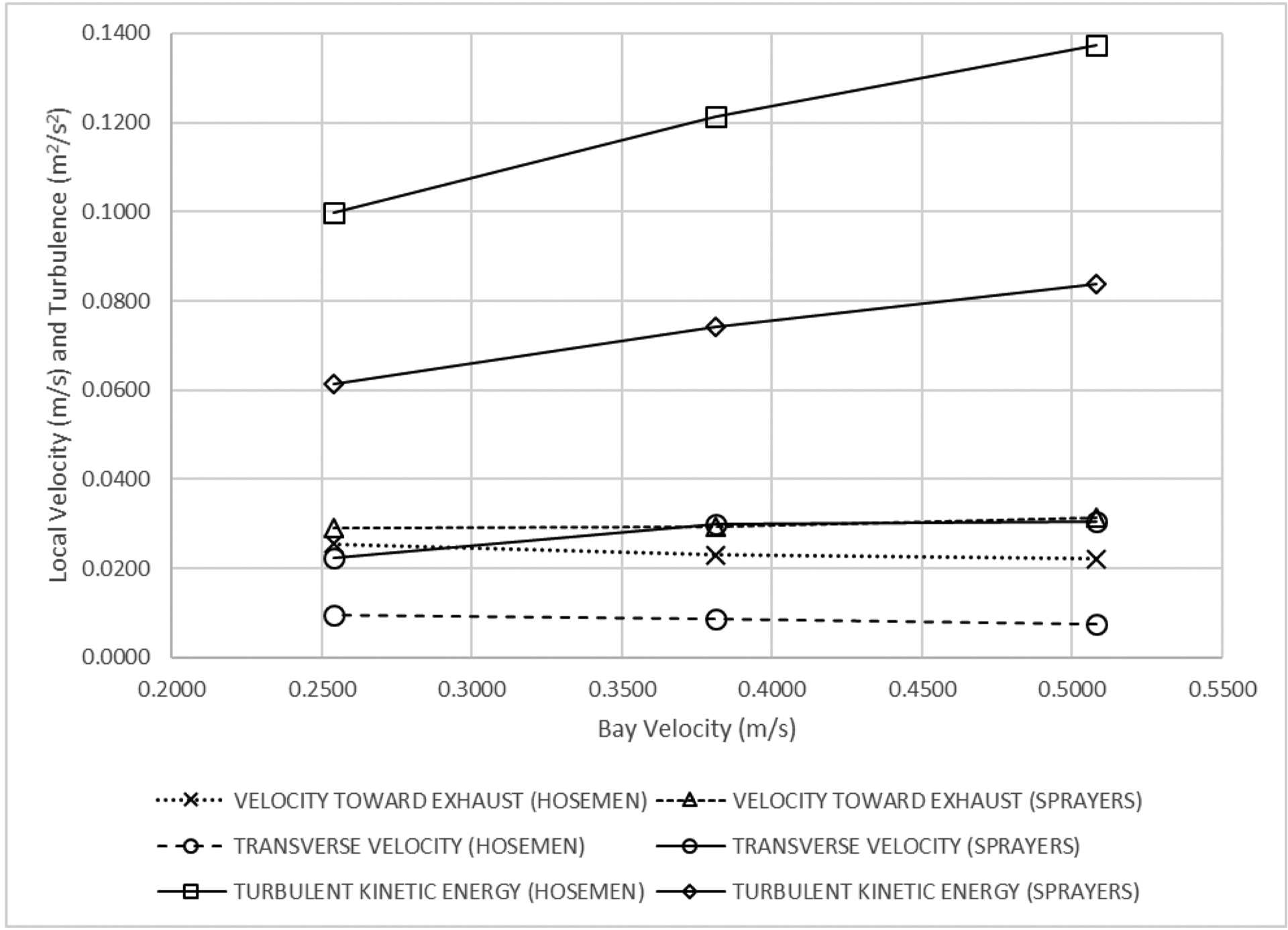
CFD simulation results for velocities and turbulent kinetic energy in the work zones of sprayers and hosemen, as a function of crossflow velocity through the bay. Transverse velocity was calculated as velocity magnitude minus velocity toward exhaust.

TABLE II.

CFD Velocities and turbulence quantities near the aircraft and workers

Bay Velocity (m/s) (fpm)	Zone	Velocity Toward Exhaust (m/s)	Velocity Toward Exhaust Fine Grid (m/s)	Velocity Magnitude (m/s)	Transverse Velocity (m/s)	TKE (m2/s2)	TKE Fine Grid (m2/s2)	Turb. Reynolds Number	Y+ 1st Cell	Y+ 10th Cell
0.508	FREESTREAM	0.5127	--	0.5361	0.0234	0.00552		3253	--	--
100	HOSEMAN_PORT	0.0146	0.0146	0.0228	0.00820	0.1422	0.1420	212.8	0.5496	15.66
	HOSEMAN_STBD	0.0296	0.0297	0.0366	0.00700	0.1325	0.1323	204.6	0.6843	21.59
	HOSEMEN_AVE	0.0221	--	0.0296	0.0075	0.13731	--	208.8	0.6170	18.63
	SPRAYER_PORT	0.0429	0.0425	0.0923	0.0494	0.0373	0.0372	83.57	0.7574	22.43
	SPRAYER_STBD	0.0197	0.0198	0.0315	0.0118	0.1303	0.1302	201.6	0.6099	14.15
	SPRAYERS_AVE	0.0313	--	0.0619	0.0306	0.0838	--	142.6	0.6836	18.46
	WORKERS_AVE	0.0267	--	0.0458	0.0191	0.1106	--	175.7	0.6503	18.54
	F-18	0.1013	--	0.1371	0.0358	0.00668	--	120.6	0.6526	27.40
0.381	FREESTREAM	0.3847	--	0.4030	0.0183	0.00498	--	3161	--	--
75	HOSEMAN_PORT	0.0141	0.0141	0.0228	0.00868	0.1261	0.1259	199.2	0.5108	15.37
	HOSEMAN_STBD	0.0320	0.0320	0.0409	0.00888	0.1164	0.1163	190.8	0.6775	21.27
	HOSEMEN_AVE	0.0230	--	0.0318	0.0088	0.1212	--	195.0	0.5942	18.32
	SPRAYER_PORT	0.0387	0.0384	0.0891	0.05040	0.0326	0.0326	77.83	0.7215	19.59
	SPRAYER_STBD	0.0201	0.0200	0.0297	0.00958	0.1158	0.1157	188.7	0.5634	11.87
	SPRAYERS_AVE	0.0294	--	0.0594	0.0300	0.0742	--	133.3	0.6424	15.73
	WORKERS_AVE	0.0262	--	0.0456	0.01938	0.0977	--	164.2	0.6183	17.02
	F-18	0.0800	--	0.1190	0.039	0.00544	--	116.5	0.5859	25.49
0.254	FREESTREAM	0.2565	--	0.2714	0.0149	0.00384	--	2546	--	--
50	HOSEMAN_PORT	0.0143	0.0143	0.0220	0.00770	0.1048	0.1048	180.1	0.4649	13.59
	HOSEMAN_STBD	0.0367	0.0367	0.0481	0.01140	0.09500	0.09500	171.0	0.6730	20.94
	HOSEMEN_AVE	0.0255	--	0.0350	0.0095	0.09991	--	175.6	0.5690	17.26
	SPRAYER_PORT	0.0337	0.0335	0.0724	0.03870	0.0258	0.0258	66.87	0.6222	12.65
	SPRAYER_STBD	0.0243	0.0243	0.0304	0.00610	0.09696	0.09691	170.8	0.5356	10.95
	SPRAYERS_AVE	0.0290	--	0.0514	0.0224	0.0614	--	118.8	0.5789	11.80
	WORKERS_AVE	0.0273	--	0.0432	0.01598	0.0806	--	147.2	0.5740	14.53
	F-18	0.0726	--	0.1044	0.0318	0.00412	--	107.1	0.5310	23.65

Note: Quantities are averaged over a ten-cell boundary region surrounding each body. The freestream zone is the remaining bay volume after aircraft and worker zones have been removed.

Verification and Validation

Table II also shows that local velocities and TKEs for the original and the finer grid are nearly indistinguishable. Sufficient grid resolution in the boundary layer around the F-18 surfaces and the workers are indicated in Table II by first-cell y⁺-values all being less than one. Figure 10 shows CFD and tracer experiment concentration means across monitoring locations. To compare the predicted effects of velocity, CFD concentrations were divided by tracer gas concentration at full-flow to create a normalized reference value. Both methods showed a similar decrease in concentration when the flow was lowered from full- to 3/4-flow. Tracer experiments indicated a large increase in normalized concentration when the velocity was decreased further, from 3/4- to half-flow. In the CFD simulations, however, there appears to be no discernable difference between concentrations at 3/4- and half-flows.

FIGURE 10.

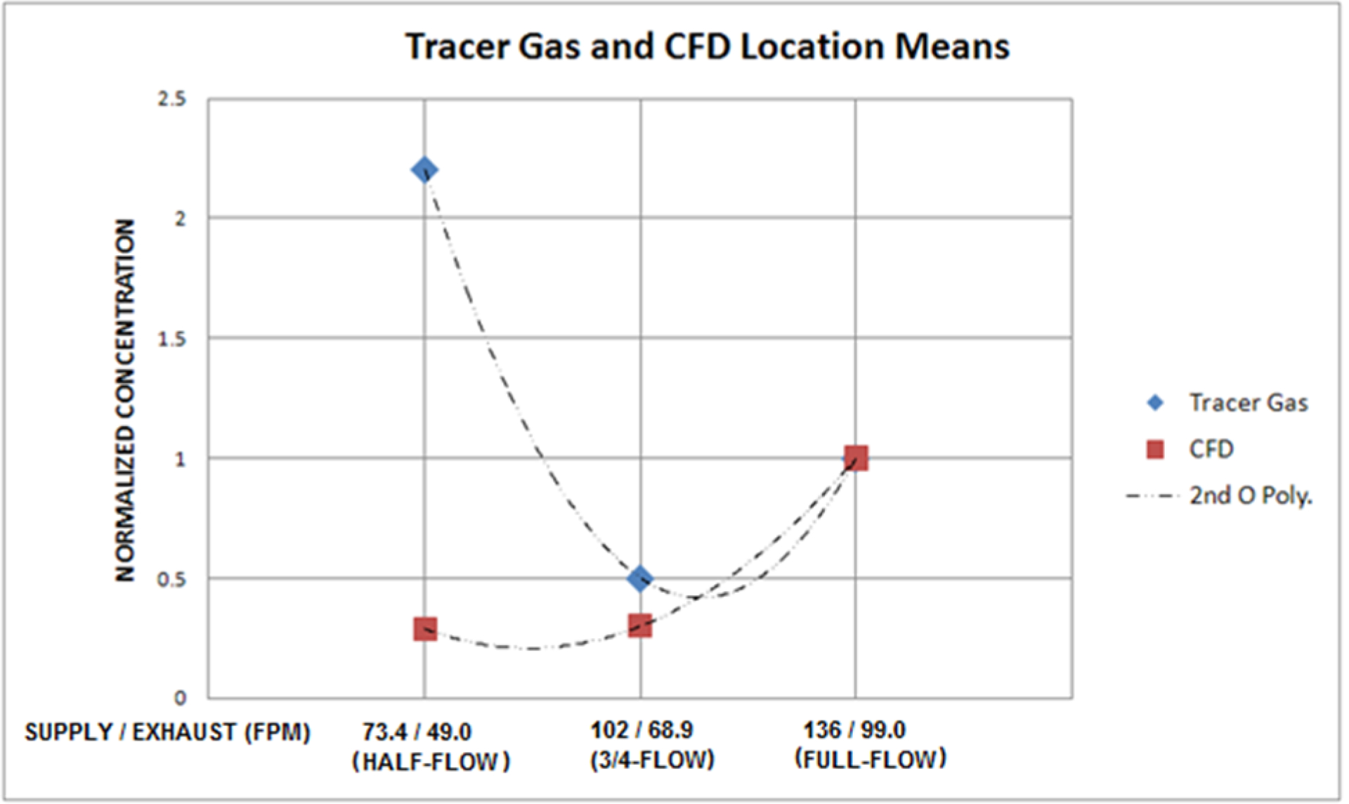
Five-location-mean concentrations for CFD simulations and tracer gas experiment means, as a function of velocity.

Thus, the CFD techniques employed here were consistent with the tracer gas results in the moderate and high ventilation velocity range and inconsistent in the low velocity range. This latter behavior, unfortunately, is commonly seen, and the remedy is computationally expensive. The k-ε turdulence models may underestimate the effect that velocity fluctuations have on contaminant transport.⁽¹⁸⁾ Because velocities varied across the real filter faces, whereas the simulation boundary conditions were uniform, it is possible that the simulations created a more effective velocity field for contaminant removal, with fewer flow reversals. However, Figure 6A shows that boundary velocities determined the flowfield at worker locations only partially.

Figure 11 shows the effect of flow reduction through multiple pair-wise comparisons. Tracer location means, in blue, along with their 95% error bars for Tukey’s studentized range HSD test, are plotted with the CFD results. Half-flow concentrations being statistically significantly higher than 3/4-flow is shown here by the confidence interval staying above zero. For the 3/4 vs. full comparison, CFD and tracer results diverge. Interestingly, all CFD predictions are at or within the 95% confidence limits for the tracer measurements.

FIGURE 11.

Flow rate comparison by CFD and tracer gas methods.

Tracer Gas Experiments

Recall that the supply/exhaust velocities in the tracer gas experiments were: full-flow, 0.706/0.503 m/s (139/99.0 fpm); 3/4-flow, 0.518/0.350 m/s (102/68.9 fpm); and, half-flow, 0.371/0.249 m/s (73.4/49.0 fpm). As shown in Table V, SF₆ concentrations at the five monitoring locations were higher for half-flow than for 3/4-flow, with statistical significance (95% confidence intervals did not overlap). No statistically significant difference was found between half-flow and full-flow or 3/4-flow and full-flow. The rate of 3/4-flow had the lowest mean concentration. This unbalanced rate created a measured hangar midpoint velocity of 0.374 m/s (73.6 fpm), whereas the half-flow and full-flow conditions produced velocities of 0.365 m/s (71.8 fpm) and 0.528 m/s (104 fpm) respectively. The closeness of the midpoint velocities for 3/4- and half-flows should not be interpreted as precisely representing the velocities through the work area, since the 16-point measurement matrix was somewhat coarse for the hangar bay crossectional area of 134 m². The velocity fields were probably better represented by considering the measured supply, midpoint, and exhaust velocities together.

DISCUSSION

Motivation for investigating the effects of relatively small changes in ventilation velocity comes primarily from the need to control exposures in this hazardous process, while a secondary consideration is energy use, in light of the fan law:

$$\frac{PW{R}_1}{PW{R}_2}={\left(\frac{Q_1}{Q_2}\right)}^3.$$ Eqn. 2

Thus, small increases (decreases) in volumetric flow rate or in velocity result in greater increases (decreases) in the rate of energy use. Furthermore, the ventilation system in the present study was well-designed and maintained, yet inadequately controlled exposures, and respiratory protection was required. OSHA regards this large facility as a “spray area,” which does not have a specific air velocity requirement, unlike a “spray booth” or “spray room,” which requires 0.508 m/s (100 fpm).⁽⁷⁾ Because balanced ventilation adhering to 29 CFR 1910.94 (100 fpm) would still need supplementation with appropriate respirators, the level of protection engineering controls must deliver is best defined by the aircraft painting section of the OSHA hexavalent chromium standard. Controlling Cr[VI] concentrations below 25 μg/m³, as an 8-hr TWA, is probably a more applicable performance metric than maintaining an air velocity of 0.508 m/s (100 fpm). Cr[VI] exposures for aircraft painting seem to be near or above the OELs, making Cr[VI] a sensitive indicator of engineering control performance, whereas HDI exposures in the surveys reported here were below the OELs.

During the follow-up survey, airflow measured in each bay was within 25 fpm (0.127 m/s) of the 100 fpm OSHA criterion at the mid-hangar location, with an aircraft present. Supply and exhaust flow rates were well-balanced in Bays 1 and 6, but were poorly balanced in Bays 4 and 5. The imbalance might have resulted from exhaust filters visibly coated with overspray.

The isocyanate, hexavalent chromium and total particulate results that compare the initial and follow-up surveys do not show a consistent relationship between ventilation velocity and contaminant concentration. Depending on the statistical test used, an increase in exposure in the far field zone occupied by hosemen could be observed. It is clear that any ventilation rate effect differentiating moderate and high velocities was not large compared to other sources of concentration variability. Considering Table V, a reasonable interpretation is that airflow of 0.406 m/s (80.0 fpm) was not less protective than airflow of 0.528 m/s (104 fpm), under the conditions evaluated here. While there were specific contaminants and worker positions where one velocity was more protective than the other, the bigger picture seems to be that velocity in this range had little exposure impact.

Air sampling involved some uncontrolled variables. The surveys were conducted in different bays, although with very similar ventilation (Bay 6 versus combined Bays 7 and 8, and Bay 2); some samples were collected during painting of different aircraft (F-18 versus E-2 and C-2); and, somewhat different quantities of paint were used in the operations. Therefore, changes in contaminant concentrations cannot be attributed solely to the ventilation system modification. However, velocity effect comparisons were made only for F-18 painting.

CFD simulations and tracer experiments both indicated a substantial increase in worker protection when the ventilation velocity was increased from the low range, 0.254 – 0.335 m/s (50 – 66 fpm), to either the moderate range, 0.381 – 0.406 m/s (75 – 80 fpm), or the high range, 0.432 – 0.528 m/s (85 – 104 fpm). CFD and tracer methods were required because observation of the real paint spraying process at low velocities was not desireable. Considering moderate vs. high ventilation, the results indicated either moderate ventilation being slightly more protective than high, or the lack of a discernable difference.

The tracer and CFD results indicated that the range 0.254 to 0.335 m/s (50 to 66 fpm) was clearly too low, and a physical interpretation is that the flow was subject to meandering. A reasonably unidirectional flow path should be the goal in crossflow ventilation. Exposure reduction evident for hosemen but not for sprayers, in the range 0.432 to 0.528 m/s (85 to 104 fpm) compared to 0.381 to 0.406 m/s (75 to 80 fpm), may indicate that increasing turbulence promoted isotropic contaminant transport, and the CFD results in Figure 8 do show TKE increasing with velocity.

It may be the case that in the higher bay velocity range, the benefit of shorter average contaminant residence times was undone by this eddy diffusivity effect on the near-field occupied by the sprayers. Apparently in the far-field occupied by the hosemen, shorter average residence times at the higher velocity was more important. However, local work zone velocities being nearly constant over a doubling of the upwind velocity (Figure 8) implies that the concentration effect of upwind velocity in this range is very small, while the concentration effect of local work zone velocity remains untested. Another possibility is that specific sampling locations had more favorable exposure reduction-- for one velocity or another-- due to effects of worker movement on the local flowfield that were not accounted for in the CFD models. What is clear is that upstream velocity was a poor predictor of local velocities in work zones.

CONCLUSION

Crossflow ventilation velocity of approximately 0.254 m/s (50 fpm) was less effective at exposure reduction than either 0.381 or 0.508 m/s (75 or 100 fpm). No general difference was clearly discernable between 0.381 and 0.508 m/s (75 and 100 fpm), although local exposures did vary with velocity. That a maintained linear rate of approximately 0.508 m/s (100 fpm) provided inadequate protection creates a caution against over-reliance on the intuitive concept that more ventilation is better. Moreover, because velocity increases lead to exponentially increased energy use, while possibly adding no protective value, flow paths that provide efficient unidirectional contaminant removal should be foundational in aircraft painting ventilation design.

REFERENCES

- 1.Bennett JS, Marlow D, Nourian F, et al. : Hexavalent chromium and isocyanate exposures during military aircraft painting under crossflow ventilation. J. Occup. Environ. Hyg 13(5):356–371 (2016). [DOI] [PMC free article] [PubMed] [Google Scholar]
- 2.U.S. Department of Health and Human Services: Preventing Asthma and Death from Diisocyanate Exposure. Centers for Disease Control and Prevention, National Institute for Occupational Safety and Health, DHHS (NIOSH) Publication No. 96–111. 1996. [Google Scholar]
- 3.U.S. Department of Health and Human Services: NIOSH ALERT: Preventing asthma and death from MDI exposure during spray-on truck bed liner and related applications. Centers for Disease Control and Prevention, National Institute for Occupational Safety and Health, DHHS (NIOSH) Publication No. 2006–149. 2006. [Google Scholar]
- 4.Vandenplas O, Cartier A, Lesage J, et al. : Prepolymers of hexamethylene diisocyanate as a cause of occupational asthma. J. of Allergy and Clin. Immunol 91:850–861 (1993). [DOI] [PubMed] [Google Scholar]
- 5.Bello D, Woskie SR, Streicher RP: Polyisocyanates in occupational environments: a critical review of exposure limits and metrics. Am. J. Ind. Med 46: 480–91 (2004). [DOI] [PubMed] [Google Scholar]
- 6.U.S. Department of Health and Human Services: “Workplace Safety and Health Topics: Hexavalent chromium.” Centers for Disease Control and Prevention, National Institute for Occupational Safety and Health. Available at: http://www.cdc.gov/niosh/topics/hexchrom (accessed: June 12, 2015). [Google Scholar]
- 7.“Occupational Safety and Health Standards, Subpart G: Occupational Health and Environmental Control, Standard 1910.94: Ventilation, Section (c)(6): Velocity and airflow requirements.” Code of Federal Regulations, Part 1910. [Google Scholar]
- 8.U.S. Department of Defense: Unified Facilities Criteria, UFC 4-211-02NF. Industrial Ventilation. Ch. 2–4.2.2, Corrosion Control and Paint Finishing Hangars. 2010. p. 12. [Google Scholar]
- 9.“Occupational Safety and Health Standards, Subpart G: Occupational Health and Environmental Control, Standard 1910.1026: Chromium (IV), part (f)(1)(ii).” Code of Federal Regulations, Part 1910. [Google Scholar]
- 10.American Conference of Governmental Industrial Hygienists (ACGIH): Industrial Ventilation—A Manual of Recommended Practice, 27th Edition. Cincinnati, Ohio: ACGIH, 2010. pp. 13–134,135. [Google Scholar]
- 11.U.S. Department of Health and Human Services: Particulates not otherwise regulated, total: Method 0500. In NIOSH Manual of Analytical Methods, 4th ed. Ashley KA (ed.). Centers for Disease Control and Prevention, National Institute for Occupational Safety and Health, DHHS (NIOSH) Publication Number 94–113. Available at: www.cdc.gov/niosh/nmam (accessed 6/12/2015). [Google Scholar]
- 12.U.S. Department of Health and Human Services: Chromium, hexavalent (by ion chromatography): Method 7605 (supplement issued 3/15/2003). In NIOSH Manual of Analytical Methods, 4th ed. Ashley KA (ed.). Centers for Disease Control and Prevention, National Institute for Occupational Safety and Health, DHHS (NIOSH) Publication Number 94–113. Available at: www.cdc.gov/niosh/nmam (accessed 6/12/2015). [Google Scholar]
- 13.U.S. Department of Health and Human Services: Isocyanates, total (MAP): Method 5525 (supplement issued 3/15/2003). In NIOSH Manual of Analytical Methods, 4th ed. Ashley KA (ed.). Centers for Disease Control and Prevention, National Institute for Occupational Safety and Health, DHHS (NIOSH) Publication Number 94–113. Available at: www.cdc.gov/niosh/nmam (accessed 6/12/2015). [Google Scholar]
- 14.Tu J, Yeoh GH, Liu C: Computational Fluid Dynamics: a practical approach. Oxford: Elsevier, 2008. pp. 263–264. [Google Scholar]
- 15.Wilcox DC: Turbulence Modeling for CFD. La Canada: DCW Industries, 1998. p. 125. [Google Scholar]
- 16.Patankar SV: Numerical Heat Transfer and Fluid Flow. New York: Hemisphere, 1980. pp. 30–39, 126–131. [Google Scholar]
- 17.U.S. Department of Health and Human Services: In-depth survey report: experimental and numerical research on the performance of exposure control measures for aircraft painting operations, part II. Centers for Disease Control and Prevention, National Institute for Occupational Safety and Health, EPHB-329–12b, 2012. Available at: www.cdc.gov/niosh/surveyreports/pdfs/329-12b.pdf (accessed 01/03/2017).
- 18.Lin C, Horstman RH, Ahlers MF, Sedgwick LM, Dunn KH, Topmiller JL, Bennett JS, Wirogo S: Numerical Simulation of Airflow and Airborne Pathogen Transport in Aircraft Cabins, Part 2: Numerical Simulation of Airborne Pathogen Transport. ASHRAE Transactions 2005, Vol.111, Part I, pp.764–768. [Google Scholar]