Abstract
The prediction of hospital patients and outpatients with suspected arboviral infection individuals in research-limited settings of the urban areas is defined as a challenging process for clinicians. Dengue, Chikungunya, and Zika arboviruses have gained attention in recent years because of the high prevalence in the society and financial burden of major global health systems. In this study, we proposed a machine learning algorithm based prediction model over retrospective medical records, which are named as SISA (the Severity Index for Suspected Arbovirus) and SISAL (the Severity Index for Suspected Arbovirus with Laboratory) datasets. Therefore, we aim to inform the clinicians about the use of machine learning with transfer learning success for diagnosis and comprehensive comparison of the classification performances over the SISA/SISAL datasets in the resource-limited settings that may cause to the small datasets of arboviral infection. In this study, Convolutional Neural Network and Long Short-Term Memory have achieved 100% accuracy and 1 of area under the curve (AUC) score, Fully Connected Deep Network has provided 92.86% accuracy and 0.969 AUC score in the SISAL dataset with transfer learning. Moreover, 98.73% accuracy and 0.988 AUC score were obtained by Convolutional Neural Network and Long Short-Term Memory for the SISA dataset. Furthermore, Linear Discriminant Analysis (shallow algorithm) has provided reaching up to 96.43% accuracy. Notably, deep learning based models have achieved improved performances compared to the previously reported study.
Keywords: Arboviral infection, Deep learning, Shallow machine learning, Transfer learning
Introduction
Recently, critical decisions of clinicians in an effective way are becoming important due to the shortage and resource-limited settings while facing with arboviral infections or Covid-19 infections [1, 2]. Levels of illness while deciding the length of patient staying and accurate prediction of hospital or outpatients are the main management of healthcare facilities. Triage of a suspicious patient with arbovirus infection is a challenging process for clinicians to determine the status of whether a patient should be hospital patient or outpatient [1, 3].
The series of potential pathogens causing analogous symptoms such as undiscerned febrile illness have a shared consensus in tropical medicine protocols. Dengue virus (DENV), Chikungunya virus (CHIKV), and Zika virus (ZIKV) are the types of Arthropod-borne viruses (arboviruses) caused by mosquito vectors (Aedesa egypti and Ae. albopictus). Clinical variables are commonly presented as myalgias, rash, arthralgias, and fever. The emergence of the DENV virus (in tropical Americas), CHIKV virus (in Saint Martin during 2013), and ZIKV virus (in Brazil during 2015) had gained international attention because of the expected transmission risk and high prevalence infections to other people in the society [1]. Between 2014 and 2018, 86,036 cases were reported as arboviral infections in Ecuador. Moreover, molecular or particular diagnostic tools (i.e., ELISA or PCR) and clinical laboratories for physicians at the outside of the urban areas are provided under the limitations or unavailable. The overall cost of the dengue illness was noted around 9 billion dollars over the healthcare system of the USA in 2013. The retrospective medical records of our study and previous reported study [1] were collected from the 543 subjects of suspected arboviral infection in Machala City, which is in southern coastal Ecuador amid November-2013 to September-2017 for model prediction. These obtained data were named as SISA (the Severity Index for Suspected Arbovirus) and SISAL (the Severity Index for Suspected Arbovirus with Laboratory) datasets. The SISA dataset was created with demographic and symptom data, and the SISAL dataset was combined with laboratory data in addition to demographic and symptom data.
Machine learning algorithms (ML) have growing attention in predicting medical records in recent years. The main aim of the machine learning algorithms is to recognize the pattern of data in accurate classification performances. In this study, Fully Connected Deep Network (FCDN), Convolutional Neural Networks (CNN), Long Short-Term Memory (LSTM), Support Vector Machine (SVM), and Linear Discriminant Analysis (LDA) techniques were used to process the datasets for predicting the case of hospitalization or not. FCDN has a wide range of uses and is the most fundamental element of deep learning. It does not make any special assumptions about data, so this network is applicable in a wide range of fields. CNN is a state-of-the-art deep learning method that outperforms shallow neural network algorithms at a high level of predictive accuracy. CNN has a diverse application domain, including image processing, natural language processing, data classification reaching to the inspired outcomes as well as using in the diagnosis of disease, and triage prediction [1, 4, 5]. LSTM is a type of Recurrent Neural Network (RNN). The design of neurons in LSTM has recurrent connections enabling the network in useful tasks via extraction attributes of sequence labeling such as medical records [6]. The kernel version of MLs can be considered as SVM and LDA in the literature [7]. These two algorithms were also implemented on SISA and SISAL datasets to gain insight into outcomes for the classification performances of kernel-based algorithms.
According to the previously reported study [1], k Nearest Neighbors, Bagged Trees, Elastic Net Regression, Random Forest, Generalized Boosting models, and neural networks were used as machine learning algorithms on both datasets (SISA and SISAL). The noted results were given between 89.8 and 96.2% (accuracy) and 0.50–0.91 (AUC score) on the SISA dataset, and 64.3–92.6% (accuracy) and 0.62–0.94 (AUC score) on the SISAL dataset, respectively. In our retrospective-based study (dataset access with “https://www.openicpsr.org /openicpsr/project/115165/version/V2/view”), multiple machine learning algorithms were trained and tested to develop robust and reference models in arboviral infection datasets for helping clinicians in the prediction of hospital or outpatient subjects. Moreover, receiver operating characteristic (ROC) curves and the area under the curve (AUC) scores were obtained and assessed in association outcomes of the MLs. It is worth noting that SISA and SISAL datasets were investigated to provide sufficient impact in literature for FCDN, CNN, LSTM with transfer learning among the arboviral infectious realm. Improved results under the limited resources and associated medical records were obtained and explored for prediction hospital person or outpatient in arboviral infection patients.
This article focuses on the introduction of the MLs with transfer learning effect to help the clinician decisions better over arboviral infections on limited setting resources and small volume datasets. More precisely, we describe the performance, characteristics, development, and evaluation of ML models that can directly assist clinicians in diagnosing arboviral infectious diseases, predicting severity, and deciding whether to hospitalize or not.
Materials and methods
Description of the dataset
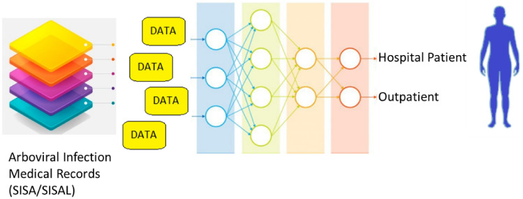
The retrospective medical records, including the SISA (Severity Index for Suspected Arbovirus) and SISAL (Severity Index for Suspected Arbovirus with Laboratory) datasets, were collected to predict the status of patients whether they should be hospital or outpatient [1]. Hence the resource-limited settings and the density of emergency departments can be arranged in an effective way for health care systems. The datasets were extracted as a part of the ongoing surveillance study at Ecuador Machala. The datasets include demographic data, past medical histories, symptom data, and laboratory outcomes for individuals with a suspected arbovirus. The SISA dataset includes 543 subjects, and 28 features of each record were estimated during the evaluation process. These features are presented under the demographic, symptom, and medical history information. Pregnancy status and laboratory results were omitted in the feature set. Furthermore, 9 records of subjects with missing information were not included in the study. As a final SISA dataset, a total of 534 records, including 59 hospital patients and 475 outpatient subjects, were used. For the SISAL dataset, 39 outpatients, and 59 hospital individuals were estimated among 98 records. Then 33 features other than pregnancy status were examined in the evaluation of this dataset [1]. Table 1 presents the list of processed features. Moreover, general schematic of the clinical decision support system based on the machine learning was shown in Fig. 1.
Table 1.
The list of processed features
| Demographic data | Presenting symptoms | Past medical history | Laboratory data |
|---|---|---|---|
| Age (years) | Temperature (°C) | Allergies (%) | Hemotocrit (%) |
| Height (cm) | Fever in past 7 days | Hypertension (%) | WBC count (cells/ML) |
| Weight (kg) | Head pain (%) | Asthma (%) | Neutrophills (%) |
| Mua circumference (cm) | Nausea (%) | Cancer (%) | Lymphocytes |
| Waist circumference (cm) | Muscle or joint pain (%) | Diabetes (%) | Platelet count |
| Gender | Rash (%) | Dengue in the household (%) | |
| Bleeding (%) | Dengua (%) | ||
| Rhinorrhea (%) | |||
| Vomiting (%) | |||
| Drowsiness or lethargy (%) | |||
| Coughing (%) | |||
| Abdominal pain (%) | |||
| Diarrhea(%) | |||
| Retro-orbital pain (%) | |||
| Positive tourniquet test (%) |
Dataset Access (https://www.openicpsr.org/openicpsr/project/115165/version/V2/view)
Fig. 1.
The schematic of the clinical-decision support system in predictions of hospital patient or outpatient for arboviral infected patients using machine learning over the SISA/SISAL medical records
Convolutional neural networks
CNN, a typical multi-layered neural network structure, is often used to analyze image-related applications [8, 9]. The basic working principle of CNN architectures can be summarized as extracting the features of the image taken from the input layer and classifying the extracted features in fully connected layers. CNNs are largely similar to feedforward neural networks. However, the main difference of CNN based machine learning models from traditional machine learning methods is that there are convolution layers in CNN that automatically extract features. CNN models consist fundamentally of convolution, pooling, and fully connected layers [8, 9].
The size of the filter and the number of maps generated are used to define the convolution layer. This layer is the fundamental unit consisting of filters that aim to extract different features related to lines, corners, and edges of input images [10]. These filters, including pixel values, are slid across the image matrix. During the sliding process, the values of the image matrix are multiplied by the values in the filter, and the values obtained are summed, and the net result is found. This process is applied to the whole image to obtain feature maps, and thereby a new matrix is created. Subsequent feature map values are calculated as given in Eq. (1) [10].
| 1 |
where is the signal of the feature map or output vector, denotes the number of elements in the time series of a signal, means the kernel or filter, and the subscripts indicate the nth vector variable.
A further important layer of CNN is the pooling layer, which takes small rectangular blocks for reducing the dimension of the outputs from the convolutional layer [8, 10]. Thus, the computational requirements are progressively mitigated, and the likelihood of overfitting is minimized. In this study, the max-pooling operation, which selects only the largest value in each feature map, is used.
The fully connected layer is a typical neural network that connects all the neurons of the previous layer to each of its own neurons. The principal aim of the artificial neural network is to combine features into more attributes in order to estimate the classes with greater accuracy. This research contains two forms of activation functions: (1) Rectified Linear Activation Unit (ReLU) and (2) Softmax [10]. ReLU performs a threshold operation for each input variable that removes negative values by setting them to zero that imparts nonlinear properties to the network architecture. Then Softmax is used to predict which class the input image (hospital patient/outpatient) belongs to according to the probability value for classes [10].
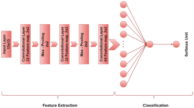
In this study, the CNN model proposed for this study has 5 learnable layers (3 convolution layers and 2 fully connected layers). The convolution layers contain three phases as convolution, ReLU, and max-pooling. The first 2 convolution layers have 32 feature maps, and the third convolution layer has 64 feature maps, respectively. The filter size is 2 × 2, and the stride size of 1 pixel is used. The convolution layers are followed by 2 fully connected layers consisting of 70 nodes and 1 node, respectively. The softmax classification layer is connected to the output of the second fully connected layer. The training process was carried out in 400 epochs. The CNN architecture used in this study is shown in Fig. 2.
Fig. 2.
CNN model architecture
Data to image conversion
In both datasets, we apply the features to CNN after converting them to grayscale images. First of all, each column in the dataset is normalized for this process. The column vector , with and its nominalized form can be represented as in equations:
| 2 |
| 3 |
Here, the normalization process of each column can be defined as follows:
| 4 |
where ai is input value in the column vector A. After the datasets are normalized as described above, the feature vector of each patient in 1 × 33 dimensions is converted to 11 × 3 matrices. Here, all values for "Laboratory Data" information in the SISA dataset are assigned to "0". Figure 3 shows sample representations created at this stage for SISA and SISAL datasets. Then, by adding “0” values to the end of the rows and columns of the matrix, 15 × 15 size greyscale representations are obtained.
Fig. 3.
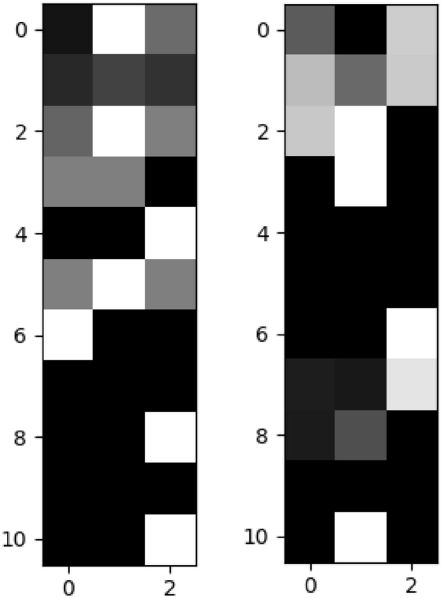
Sample Image representations of data (left: SISA, right: SISAL)
Long short-term memory network
LSTM is a special type of recurrent neural network (RNN) structure used in deep learning [11, 12]. If there is a correlation between the data memorized at different times, this is called “long-term dependency” [13]. While it is aimed to store and transmit state information of the artificial neural network while processing on arrays in RNNs, it is not possible to transmit without disturbing long-term dependencies as a result of continuous processing of state information. In other words, while short term dependencies in the array are transferred successfully, there is a problem in transferring long term dependencies. The LSTMs are a state-of-the-art technique and specifically structured to address the problem of long-term dependence [11, 13].
LSTM module consists of 3 separate gates. The names of these gates are forget, input, and output [11]. Forget gate decides how much of the information will be forgotten and how much of it should be transferred to the next stage. It has a sigmoid layer that produces a value between 0 and 1 for this process. 0 means that no part of the information will be transmitted, and 1 means that all information must be transmitted. It is possible to express the mathematical model of the forget gate as follows [11]. In general, W means the weight vector, b is the bias term, σ defines the sigmoid activation function for nonlinearity, xt is the input sequence, is the output of the neuron at time for feedback into the neuron. Moreover, define input, forget and output gate, respectively.
| 5 |
The next step is to decide what information should be stored. At this stage, firstly, the 2nd sigmoid layer, which is called the input gate, decides which values should be updated. The next tanh layer forms a vector of the new candidate values of the memory cell expressed as , and then these two operations are combined. This process is expressed mathematically as follows [11]:
| 6 |
| 7 |
After this, the new status information of the memory cell (Ct) must be calculated. In this case, the new status information of the memory cell is determined as follows [11]:
| 8 |
At the last stage, the output of the system (ht) is calculated. This is done at the output gate and the output of the system ht can be calculated as follows [11]:
| 9 |
| 10 |
The basic schematic representation of the LSTM is given in Fig. 4. In this study the LSTM model consists of 3 learnable layers. Each of the first two layers consists of 100 LSTM units. These are followed by a fully connected layer of 1 neuron. Finally, there is the softmax classification layer. For SISA and SISAL datasets, the input shape of 28 × 1 and 33 × 1 is used, respectively. The training process is carried out in 500 epochs.
Fig. 4.
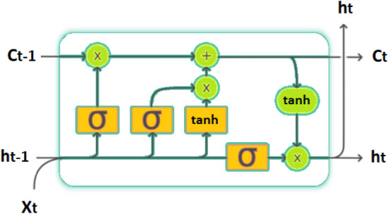
Schematic of the LSTM
Fully connected deep network
Fully Connected Deep Networks (FCDN) are the most basic elements of deep learning and have been used in a large number of applications until today. The main advantage of these networks is that they are "structure agnostic" [14]. That is, they do not make any special assumptions about the input. Being structure agnostic makes these networks applicable in a wide range of fields. However, the performance of FCDNs tends to be lower than networks adapted to the nature of the problem in a specific area [14].
FCDN is formed by the combination of a number of fully connected layers. In fact, the fully connected layer is a function from to . Here the size of each output depends on the size of each input.
Where is the input for the fully connected layer and is the i-th output of the fully connected layer, here is calculated as follows:
| 11 |
Here, wi is the learnable parameters in the network, and f is the nonlinear function. In this case, the entire output y can be expressed as:
| 12 |
Figure 5 shows a representation of the FCDN model with fully connected layers used in this study. The model consists of an input layer, three hidden layers, and an output layer. While the first hidden layer consists of 20 neurons, the second and third hidden layers consist of 10 neurons each. ReLU is used as the activation function in hidden layers. There is 1 neuron in the output layer, and the sigmoid is used as the activation function in this layer. Besides that, Adam optimizer was used in the training phase of the model.
Fig. 5.
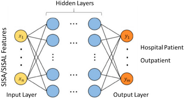
FCDN model architecture with fully connected layers
Support vector machine
Support Vector Machine is a powerful machine learning algorithm that is characterized as a kernel-based classifier [10]. SVM has many diverse application fields extending from biosignal classification to pattern recognition. The approach in this supervised learning algorithm is based on determining the support vectors to discriminate decision boundaries named as a hyperplane. The nearest support vectors extending to both sides of hyperplanes are called margin. The gaining of generalization ability in SVM is to find maximum margin and optimal hyperplane. The mathematical background of SVM is represented in Eqs. (13–15) [10].
| 13 |
| 14 |
| 15 |
where in Eqs. 13–15, defines the hyperplane, is the localized hyperplane, and means the orientation. Learning rate, initializations, and convergence checking are not required in SVM while carrying out the parameters. Figure 6 shows the fundamental notions of SVM structure and classification process [10].
Fig. 6.
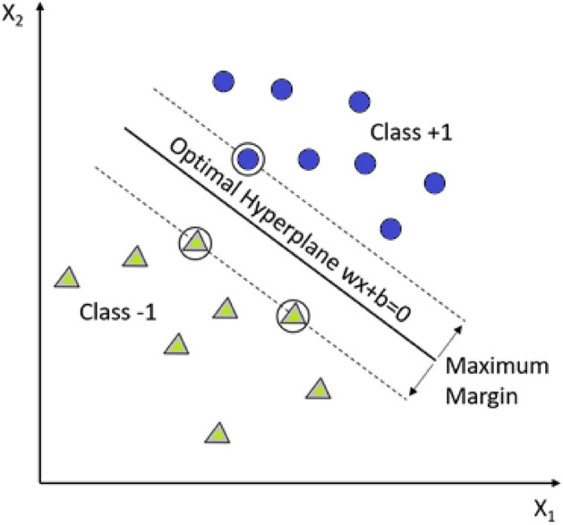
SVM and maximizing the hyperplane margin for data classification
Linear discriminant analysis
Linear Discriminant Analysis is derived from the Kernel Fisher Discriminant analysis and uses a kind of projection technique by reducing the data dimension [15]. Maximizing the between-class distance and minimizing within-class distance is the main aim of LDA. When the classes of the samples are defined as C1 and C2, and LDA aims to find the projection direction (w) for maximum separability of the spatial pattern as possible. Mathematical formulations of LDA can be represented in Eqs. (16–18).
| 16 |
where x (data samples) are projected onto w, and the LDA representation is shown in Fig. 7 [7]. Where to stands for means of samples in C1 before and after, respectively. Hence, and . Then and have a similar manner for C2. Scattered samples around the means are and [7]. When the training sample is defined as :
| 17 |
| 18 |
where and are called as between-class scatter matrix and within-class scatter matrix in , respectively [7].
Fig. 7.
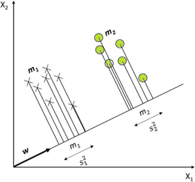
The task of classification in LDA via the projection of data samples
Performance evaluation metrics
In our retrospective-based study, several appropriate metrics were used to evaluate the performances of machine learning algorithms for prediction hospitalization or outpatient in arboviral infection patients over the medical records. These performance evaluation metrics can be listed as k-fold cross validation, classification accuracy (ACC), sensitivity (SENS) and specificity (SPEC) analysis, receiver operating characteristics (ROC), area under the curve (AUC).
SISA and SISAL datasets for traditional validation were partitioned to 70 (training)—30% (test) and 85% (training)—15% (test), respectively. Moreover, the k-fold cross-validation method was used to achieve unbiased training/testing data division besides the traditional validation. This approach is a common methodology used for training and test data separation [16, 17]. The aim of this process is to submit each data in the prepared dataset for testing and training [16]. In this technique, the dataset is split into k-subsets by the stated k number. The classifier is trained with k − 1 subsets, and an error value is calculated by testing the classifier with the remaining subset. The process is repeated k times so that each sample in the dataset is both trained and tested. The error is determined by taking the average value of the errors obtained for each subset [16, 17].
Formulas used to calculate classification accuracy, which can be considered a starting point for performance evaluation are given as follows [10, 18]:
| 19 |
| 20 |
| 21 |
where N denotes the classified (test) dataset, cn is the class of the value of n, Estimate(n) refers to the classification result of n, and the k value is the k-fold cross-validation parameter utilized in algorithms.
In order to make robust predictions, we need to determine whether the proposed algorithm is a sufficiently successful model. Accuracy alone is not a satisfactory parameter when determining the adequacy of the model. From this perspective, the terms sensitivity and specificity should also be defined. The term "sensitivity" refers to the ratio of correctly predicted true positives, while the term "specificity" is the ratio of correctly predicted true negatives. The equations of sensitivity and specificity are given as follows [10]:
| 22 |
| 23 |
where;
True Positive (TP): The number of hospitalization decisions for patients who need to be hospitalized,
True Negative (TN): The number of outpatient decisions for outpatients,
False Positive (FP): The number of hospitalization decisions for outpatients,
False Negative (FN): The number of outpatient decisions for patients who need to be hospitalized.
Thanks to the ROC and AUC evaluation metrics, it is possible to visualize the performance of the classifiers. The ROC curve, a two-dimensional plot that shows whether a classifier is successful, is widely used in diagnostic researches [19]. The ROC curve is plotted with the false positive rate (X axis) and the true positive rate (Y axis). At the end of the analysis, the value specified as AUC represents the area under the ROC curve and higher values imply better classifier performance. The calculated AUC value will always be across the interval [0, 1], and values greater than 0.6 are considered "acceptable discrimination" [19].
Experimental evaluation
The primary purpose of this study is to help clinicians for evaluating the hospitalization status of people with the suspected arboviral virus using machine learning algorithms. The system has two outcomes, namely, outpatient or hospitalized treatment. Thus, it is aimed to make the most accurate decision in a short time by providing a system that will help physicians make decisions, especially in regions with limited resources. Although the distinct target of the proposed approach is resource-constrained regions, it can also be used to assist decision-makers in situations that impose sudden burdens on global health systems such as the Covid-19 pandemic. Accordingly, tests were carried out on two separate datasets named SISA and SISAL introduced in the above sections.
Both datasets have their limitations. The first is that the SISA dataset is an extremely class imbalance. If the imbalance between classes is too high, machine learning algorithms generally perform poorly for the minority class, resulting in a low sensitivity problem [20]. Moreover, this is a common problem in medical datasets. Another problem is that the SISAL dataset is relatively small. In this case, it makes it difficult to use methods that are applied very successfully on many problems, such as deep learning algorithms. Although deep learning algorithms have been successfully applied in a wide range of fields, they require relatively more data compared to traditional machine learning algorithms [9, 21, 22].
In this study, an approach based on deep learning and transfer learning methods is used to overcome the problems mentioned above. Accordingly, tests are carried out with FCDN, CNN, and LSTM deep learning models. Also, the results obtained with the more traditional methods SVM and LDA models are evaluated. Besides, a comparison is presented with the previous study [1] in the same datasets. In the comparison of the proposed approach, classification accuracy (ACC), specificity (SPEC), sensitivity (SENS), and area under the curve (AUC) values were used as metrics.
Table 2 shows the results obtained using tenfold cross validation on the SISA dataset. The best results for all benchmarks were obtained with the LSTM model. In LSTM model, for ACC, SENS, SPEC and AUC 98.70%, 91.23%, 99.47% and 0.988 values were obtained, respectively. SVM and LDA produced almost the same ACC values. ACC for SVM was 96.06%, while it was 96.08% for LDA. The CNN model, on the other hand, exhibited some success over SVM and LDA with 96.85%. For SPEC values, very close values were obtained between 97.53% and 99.47% in all models. With FCDN, scores of 97.59%, 82%, and 99.18% were obtained for ACC, SENS, and SPEC, respectively. In AUC values, deep learning models performed better than traditional methods. SENS value in SVM and LDA was 76% and 81%, respectively. Here, CNN improved 9.74% compared to LDA, while this rate was 10.23% for LSTM. Deep learning models can automatically learn the features needed for tasks such as classification and detection from data [8, 9]. Thus, it extracts useful features from information such as symptom data, demographic data, and historical medical data and learns their relationship with the hospitalization state. Therefore, deep learning works better than traditional machine learning methods [10].
Table 2.
SISA tenfold cross-validation results
| SVM | LDA | FCDN | CNN | LSTM | |
|---|---|---|---|---|---|
| ACC | 96.06 | 96.08 | 97.59 | 96.85 | 98.70 |
| SENS | 76.0 | 81.0 | 82.0 | 90.74 | 91.23 |
| SPEC | 98.52 | 97.91 | 99.18 | 97.53 | 99.47 |
| AUC | 0.956 | 0.963 | 0.981 | 0.981 | 0.988 |
Table 3 shows the classic validation results of the SISA dataset. Here, 85% of the data is used for training, and the remaining 15% is used for testing. The same values were obtained for all benchmark metrics except for the slight difference in AUC for SVM and LDA. ACC for these two models was 94.94%. On the other hand, CNN and LSTM achieved a 3.79% improvement in ACC, reaching 98.73%. FCDN achieved a 2.53% improvement in ACC compared to SVM and LDA. With FCDN, the ACC value was obtained at 97.47%. For CNN and FCDN, there was 5.71% increase in SENS compared to traditional methods, and a result of 85.71% was obtained. However, a 20% improvement was achieved for LSTM, resulting in a 100% SENS value. Also, the SENS value of LSTM increased by 8.77% compared to the tenfold validation score. This may be because the minority class is better adjusted in classical validation [20]. However, ACC value for SVM, LDA, and FCDN is somewhat low compared to tenfold validation results. In this case, it can be interpreted that the adjustment in the minority class negatively affects the performance of SVM, LDA, and FCDN. CNN provides the best score for SPEC with 100%, followed by LSTM and FCDN with 98.61%. Similar values were obtained for AUC in all models.
Table 3.
SISA 85–15 classic validation results
| SVM | LDA | FCDN | CNN | LSTM | |
|---|---|---|---|---|---|
| ACC | 94.94 | 94.94 | 97.47 | 98.73 | 98.73 |
| SENS | 80.0 | 80.0 | 85.71 | 85.71 | 100 |
| SPEC | 98.44 | 98.44 | 98.61 | 100 | 98.61 |
| AUC | 0.985 | 0.984 | 0.976 | 0.988 | 0.988 |
As a result, compared to tenfold validation, in the traditional validation process, LSTM provided a significant improvement in SENS versus an acceptable small drop in SPEC. The reduction in the number of FN (The number of outpatient decisions for patients who need to be hospitalized) here is much more critical in preventing situations that could have fatal consequences. While doing this, it is very important that SPEC values in both tables are better than traditional methods in terms of preventing the waste of resources. LSTM model gives much better results considering the results of the previous study [1] on these datasets, Tables 2 and 3. LSTM is essentially a Recurrent Neural Network (RNN) type. RNN has a looped neural network structure designed for processing sequential data such as health records. Thanks to the loop, unlike CNN and FCDN structures, it takes into account not only existing inputs but also historical information [12, 13]. This is similar to looking at past records when evaluating patients' current status [20]. There is an important restriction for RNNs called “long ‐ term dependency” at this point. In case the size of the sequential data increases, it becomes difficult to reach important information in the early period. LSTM overcomes this problem thanks to its special units. Storing both long-term and short-term dependencies makes LSTM models much more successful on sequential data. For many real-world problems, the inputs or outputs do not have sequences in most cases. However, an important point to notice is that even if your inputs and outputs are fixed vectors, this powerful formalism can be used to process sequentially [23, 24].
Table 4 shows the tenfold validation results for the SISAL dataset. ACC values of 94% and 93% were obtained for SVM and LDA, respectively. However, the ACC values of CNN and LSTM models trained directly with the SISAL dataset without transfer learning (TL) are significantly lower compared to traditional machine learning methods. The main reason for this situation is that the number of samples in the SISAL dataset is much lower compared to the SISA dataset. Although deep learning models have been used successfully in many different tasks, they need relatively more data [9, 21, 22]. Accordingly, the small size of the SISAL dataset has caused the performance values to drop significantly. The FCDN value obtained without transfer learning is also lower than SVM and LDA. When compared to CNN and LSTM, it has approximately 7% better performance. Consisting of a small number of layers and neurons, narrow FCDNs are generally sufficient to solve many problems in most cases and are successful on small-sized datasets [25]. However, TL approaches offer very serious opportunities in case the data size is low [9]. Therefore, before training deep learning models with SISAL dataset, we train with SISA dataset. Input shapes are set in the same way in both datasets. However, laboratory data values in the SISA dataset are taken as “0” since they are found in a small number of samples. FCDN, CNN, and LSTM models are first trained with the SISA dataset. The values obtained here constitute the starting weights of the model. Afterward, training is carried out again with the SISAL dataset. After the TL process, the CNN model's ACC value increased from 79.9 to 96%, while in the LSTM model it increased from 80 to 97%. The performance of the FCDN model increased from 87 to 92%. TL approach significantly increases classification performance for all deep learning models. However, the performance of the FCDN model is slightly lower than other models. While FCDNs are structure agnostic, which makes them widely applicable, in most cases they perform less than special-purpose networks [14]. The values obtained with LSTM and CNN models after TL on the SISAL dataset are better than traditional machine learning models, similar to Table 2 results. Here, too, it was provided by the highest ACC in the LSTM-TL model. CNN-TL and LSTM-TL models for SENS performed quite similarly with 98.55% and 98.39%, respectively. On the other hand, in SVM and LDA, 95% and 93.33% values were obtained for SENS, respectively. As in the SISA dataset, LSTM and CNN models have also increased SENS values here. The highest performance for SPEC was achieved with LSTM-TL model with 94.74%. The SPEC value of the CNN-TL model was 90.32%, slightly below SVM and LDA. The highest values in AUC values were provided by CNN-TL and LSTM-TL models with 0.981. Figure 8 shows the performance of machine learning algorithms for SISAL dataset with tenfold validation.
Table 4.
SISAL tenfold cross-validation results
| SVM | LDA | FCDN | FCDN (TL) | CNN | CNN (TL) | LSTM | LSTM (TL) | |
|---|---|---|---|---|---|---|---|---|
| ACC | 94.0 | 93.0 | 87.0 | 92.0 | 79.9 | 96.00 | 80.0 | 97.0 |
| SENS | 95.0 | 93.33 | 84.13 | 93.33 | 78.26 | 98.55 | 98.41 | 98.39 |
| SPEC | 92.50 | 92.50 | 91.89 | 90 | 83.87 | 90,32 | 48.65 | 94.74 |
| AUC | 0.963 | 0.942 | 0.829 | 0.902 | 0.889 | 0.981 | 0.891 | 0.981 |
Fig. 8.
Performance of machine learning algorithms for SISAL with tenfold validation
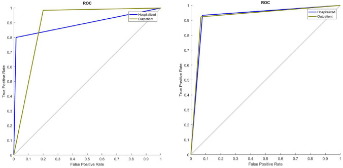
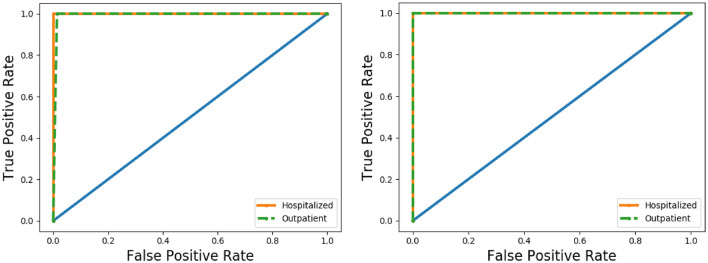
Table 5 shows the classic validation results of the SISAL dataset. Here, 70% of the data was used for education, and the remaining 30% was used for testing. The ACC values of LSTM and CNN models used without TL have remained at a very low value, 75%. The performance of FCDN without TL is better than LSTM and CNN models with ACC 85.71%. However, with the TL transaction and much better adjustment of the distribution of the minority class, both CNN-TL and LSTM-TL were successfully implemented over the all test data and was provided an ACC value of 100%. Figure 9 and 10 show the ROC curves for SISA and SISAL datasets obtained with SVM and LSTM, respectively. The highest circumstance of performances with TL (100% accuracies) was obtained by CNN and LSTM deep models in SISAL. Although small datasets are known to tend to reach overfitting situation in deep models, the same small datasets also have the potential to achieve higher predicted accuracy with pre-trained deep models with a transfer learning strategy in recent years [14, 25–27]. However, a relatively lower accuracy (< 100%) could be calculated if the dataset volumes and features were higher. The small datasets tend to reach high accuracy with shallow algorithms (SVM and LDA) compared to the deep learning algorithms [25]. The classification process has made by linear/quadratic kernels and projection methods in SVM and LDA, respectively. This truth was verified and can be observed in Tables 4 and 5 (for small SISAL dataset) if transfer learning impact is neglected on deep models.
Table 5.
SISAL 70–30 classic validation results
| SVM | LDA | FCDN | FCDN-TL | CNN | CNN (TL) | LSTM | LSTM (TL) | |
|---|---|---|---|---|---|---|---|---|
| ACC | 92.86 | 96.43 | 85.71 | 92.86 | 75.0 | 100.0 | 75.0 | 100.0 |
| SENS | 93.33 | 100 | 80.0 | 93.33 | 80.0 | 100.0 | 86.67 | 100.0 |
| SPEC | 92.31 | 92.31 | 92.31 | 92.31 | 69.23 | 100.0 | 61.54 | 100.0 |
| AUC | 0.974 | 0.985 | 0.895 | 0.969 | 0.821 | 1 | 0.733 | 1 |
Fig. 9.
ROC curves of SVM algorithms for SISA (left) and SISAL (right) classic validation datasets
Fig. 10.
ROC curves of LSTM algorithms for SISA (left) and SISAL (right) classic validation datasets
It is quite clear that deep learning models are successful in deciding the hospitalized status of individuals with a suspected arboviral virus on both datasets. However, the LSTM model was much more stable in all tests and showed high performance. It also achieved a significant improvement compared to the best SISA (ACC: 96.2%, AUC: 0.9) and SISAL (ACC: 92.6%, AUC: 0.94) reported in research paper [1]. In addition, the LSTM model proved to be much more robust to the class imbalance problem. This is very important in terms of reducing critical errors that may arise from low SENS values. High SPEC values are also very valuable in terms of preventing possible resource waste. In addition to these, deep learning models have achieved successful results with the TL approach on the low-size SISAL dataset. Although deep learning models generally require large data, they also provide very successful results on very small datasets, especially with TL [14]. Successful results of the TL approach are promising in future studies, as this method can be applied among different diseases with similar symptoms. In other words, data obtained from one disease information can be used for another disease that does not have much data.
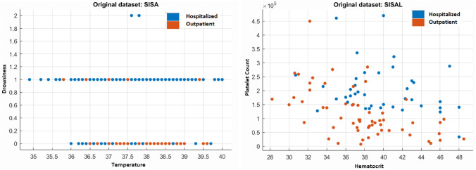
Furthermore, according to reported previous research paper about arbovirus [1], the highest variable influences for the prediction of hospital subjects and outpatients were remarked as the symptoms of drowsiness, bleeding, vomiting, and temperature for SISA. Besides, for the SISAL dataset, lower hematocrit and platelet counts were observed in the hospital individuals compared to outpatients [1]. Temperature vs. drowsiness (SISA) and hematocrit vs. platelet count (SISAL) predictors were observed to represent the effects of these properties on the prediction by creating scatter plots, as shown in Fig. 11. The relationship between the variables confirms that the two classes are almost easily distinguishable in the scatter plot diagrams.
Fig. 11.
Scatter plot representation for the highest variable influences in SISA and SISAL predictors
The level of statistical significance (p-value) is an important parameter for decision making in medicine. Hence, the features of 9–20 except feature-12 and feature-19 show the highly significant different (p-value < 0.001) in the SISA dataset. These features include head pain, nausea, muscle or joint pain, bleeding, rhinorrhea, vomiting, drowsiness or lethargy, coughing, abdominal pain, retro-orbital pain, respectively. Moreover, the feature-7 (temperature) has significantly different value (p-value = 0.013). The other features present no significant difference (p-value > 0.05).
In SISAL dataset, there are significant difference (p-value < 0.05) in the feature-6 (waist circumference), feature-7 (temperature), feature-9 (head pain), feature-10 (nausea), feature-11 (muscle or joint pain), feature-13 (bleeding), feature-16 (drowsiness or lethargy), feature-17 (coughing), feature-19 (diarrhea), feature-20 (retro-orbital pain), feature-21 (positive tourniquet test), feature-22 (hematocrit) and feature-26 (platelet count) according to the SISAL dataset predictors. Then the other features have no significant difference at the p-value (>0.05).
Discussion
The purpose of this retrospective study is to enlighten to the clinicians about the ML performances via developing a robust and effective prediction system using the ML models over the predictors of medical records (SISA and SISAL datasets). The decision is to identify for hospital patients or outpatients with arboviral infection in resource-limited settings of rural locations. In view of these limitations, investigated predictors include demographic data, symptom data, and laboratory data [1]. The constructed prediction model is based on FCDN, CNN, LSTM, SVM, and LDA algorithms among the MLs.
It is a fact that deep learning models tend to achieve more effective results with optimum solution in large datasets. However, large datasets (such as SISA/SISAL medical records) are not available or can be scarce in limited-resource settings for clinicians especially such as arboviral diseases [1]. In such cases, pre-training and transfer learning can be a reasonable choice in deep learning models with small datasets [14, 25–27]. Then these deep learning models can generalize problems with fine-tuning and can produce significant advanced performances better than shallow algorithms implemented by the previous report [1, 14, 25–27]. As our observation is the same with this truth. According to the results, LSTM and CNN with transfer learning (TL) have achieved better performances than traditional (shallow) kernel-based algorithms (ACC = 92.86% for SVM and ACC = 96.43% for LDA) reaching up to the 100% ACC and AUC of 1 in SISAL dataset for traditional validation. Using pre-trained models of CNN-LSTM with transfer learning effect has provided significant increments (ACC = 16.1–25, AUC = 0.09–0.267) on the lack of labeled SISAL datasets in terms of the performances of MLs as in the boosting strategy literature [14, 25–27]. TL approach has also increased the performance of the FCDN model. However, this rate of increase is lower compared to CNN and LSTM (Table 6).
Table 6.
The statistical distribution of the SISA and SISAL datasets
| SISA dataset (n = 534) | ||||||||||||||
|---|---|---|---|---|---|---|---|---|---|---|---|---|---|---|
| Par./Fea | 1 | 2 | 3 | 4 | 5 | 6 | 7 | 8 | 9 | 10 | 11 | 12 | 13 | 14 |
| std | 17.03 | 0.50 | 23.12 | 22.42 | 5.67 | 17.63 | 0.83 | 0.24 | 0.45 | 0.51 | 0.44 | 0.47 | 0.27 | 0.44 |
| p-value | 0.781 | 0.244 | 0.106 | 0.550 | 0.481 | 0.070 | 0.013 | 0.361 | 1e3 | 0.001 | 0.001 | 0.087 | 0.001 | 0.001 |
| Par./Fea | 15 | 16 | 17 | 18 | 19 | 20 | 21 | 22 | 23 | 24 | 25 | 26 | 27 | 28 |
|---|---|---|---|---|---|---|---|---|---|---|---|---|---|---|
| std | 0.46 | 0.43 | 0.47 | 0.52 | 0.41 | 0.51 | 0.83 | 0.41 | 0.28 | 0.22 | 0.18 | 0.27 | 0.39 | 0.47 |
| p-value | 0.001 | 0.001 | 0.001 | 0.017 | 0.225 | 0.001 | 0.821 | 0.590 | 0.57 | 0.331 | 0.243 | 0.328 | 0.458 | 0.915 |
| SISAL dataset (n = 98) | ||||||||||||||
|---|---|---|---|---|---|---|---|---|---|---|---|---|---|---|
| Par./Fea | std | p-value | Par./Fea | std | p-value | Par./Fea | Std | p-value | Par./Fea | std | p-value | Par./Fea | std | p-value |
| 1 | 13.86 | 0.655 | 9 | 0.50 | 0.001 | 17 | 0.37 | 0.044 | 25 | 17.36 | 0.278 | 33 | 0.47 | 0.579 |
| 2 | 0.50 | 0.266 | 10 | 0.47 | 0.001 | 18 | 0.48 | 0.257 | 26 | 96,064 | 0.001 | |||
| 3 | 15.85 | 0.766 | 11 | 0.50 | 0.001 | 19 | 0.44 | 0.002 | 27 | 0.44 | 0.604 | |||
| 4 | 19.29 | 0.988 | 12 | 0.38 | 0.682 | 20 | 0.50 | 0.001 | 28 | 0.26 | 0.337 | |||
| 5 | 5.08 | 0.665 | 13 | 0.38 | 0.010 | 21 | 0.86 | 0.033 | 29 | 0.14 | 0.778 | |||
| 6 | 18.53 | 0.173 | 14 | 0.30 | 0.007 | 22 | 4.57 | 0.029 | 30 | 0.20 | 0.227 | |||
| 7 | 0.96 | 0.018 | 15 | 0.50 | 0.035 | 23 | 4536 | 0.178 | 31 | 0.10 | 0.428 | |||
| 8 | 0.17 | 0.827 | 16 | 0.50 | 0.001 | 24 | 21 | 0.349 | 32 | 0.38 | 0.212 | |||
Where Par. defines the statistical parameters, Fea. shows the features of the dataset; std stands for standard deviation. If p-values are 0,001, this means p < 0,001. Mann–Whitney U test was used for statistical comparison of hospital patient and outpatient according to the features (Significant at p-value < 0.05 and No Significant at p-value > 0.05). (The details of the SISA and SISAL datasets’ features can found in https://www.openicpsr.org/openicpsr/project/115165/version/V2/view and in [1] reference)
When TL is not used, its performance on very small SISAL dataset is better than CNN and LSTM models. Hence, the potentials for applying deep learning with TL over the small datasets (SISA/SISAL datasets) has been shown in clear. In addition to this, catastrophic forgetting in machine learning is an inevitable problem to construct a general learning system with TL without losing old task ability for sequential tasks, especially in changing goals [28–30]. Firstly, the advantage is for deep models that our goals (hospital patient/outpatient) are the same to construct robust models with TL. However, this inevitable problem has been handled to reduce with fine-tuning (early stoped of training), rehearsal, sharp activation functions (applied ReLU), well-balanced sets (used with tenfold cross-validation and 70–30 classic validation), hyper-parameters with lower learning rate (used Adam Optimization with low learning rate around 0.001), max-pooling operation in CNN (implemented 2 layers) and employing difficult tasks (leading to less forgetting and leading to better generalization) strategies [28–31].
The last option about the difficult task was that the SISAL dataset includes laboratory predictors in addition to the demographic data, symptoms, and past medical history. Hence training a hard task later with more predictors in a sequence task during/after TL may have caused better generalization because it can cover more error-surfaces [28–31]. All these effects might have reduced the catastrophic forgetting without losing of generalization ability and have provided higher outcomes with TL (in Tables 4 and 5). Furthermore, the previously reported study outcomes were summarized and compared with our proposed study in Table 7.
Table 7.
Comparison performances with related previous study
| Methods | Performance results | |
|---|---|---|
| Reported Study related to the SISA/SISAL [1] | Generalized boosting model elastic net neural networks logistic regression kNN random forest bagged trees |
For SISA: ACC: 53.5–92.9% AUC: 0.51–0.94 For SISAL: ACC: 64.3–92.6% AUC: 0.62–0.94 |
| Our study |
SVM LDA CNN or CNN + TL LSTM or LSTM + TL FCDN or FCDN + TL |
For SISA: ACC: 94.94–98.73% AUC: 0.956–0.988 For SISAL: ACC: 75–100% AUC: 0.733–1 |
Generally, the rule of thumb for evaluating the AUC scores addresses that prediction and diagnostic ability of MLs have outstanding (AUC > 0.9) and excellent discrimination (0.8 ≥ AUC > 0.7) if the AUC scores range between the stated values [19]. From this point of view, AUC scores associated with SENS and SPEC values in all datasets (both for tenfold and traditional validation) have been obtained greater than 0.8 for all MLs except LSTM (AUC = 0.733). The ROC curves approved as the gold standard [19]. Then these curves have also consistent with SENS, SPEC values, and AUC scores for both SVM and LSTM. Furthermore, SISA results also suggest improved outcomes (reached up to the 98.73% ACC for CNN and LSTM) compared to the previous reported study [1].
Conclusion
The expectation of these improved outcomes aims to implement and to compare deep learning (FCDN, CNN, and LSTM) and kernel-based algorithms (SVM and LDA) over the arboviral infection records as a clinical-decision support system. Hospital systems, payers, and regulators have taken into account reducing the length of stay (LOS) and early admission with an uncertain utility [27, 32]. Hence, to be improved the performance of healthcare systems, these model-based algorithms can effectively be used when deciding accurately on the condition of hospital subjects and outpatients in arboviral infections. Moreover, it is imperative to diagnose these patients early. Hence these machine learning-based prediction models may also provide to reducing the time of triage and financial burdens at the admission level over the clinical characteristics [1, 32, 33]. In addition to helping decision of hospitalization status, neurological disorders caused by arbovirus infections may be enlightened, especially by using deep learning and transfer learning models for hospital scene and clinician [34, 35]. Future research using our model-based approach could prospectively analyze patients with Covid-19 and stratify them according to risk factors whether a patient should be hospital person or outpatient [2, 32].
Funding
There is no funding for this research study.
Declarations
Conflicts of interest
The authors declare that they have no conflict of interest.
Footnotes
Publisher's Note
Springer Nature remains neutral with regard to jurisdictional claims in published maps and institutional affiliations.
References
- 1.Sippyid R, et al. Severity index for suspected arbovirus (SISA): machine learning for accurate prediction of hospitalization in subjects suspected of arboviral infection. PLoS Negl Trop Dis. 2020;14(2):1–20. doi: 10.1371/journal.pntd.0007969. [DOI] [PMC free article] [PubMed] [Google Scholar]
- 2.Kuniya T. Prediction of the epidemic peak of coronavirus disease in Japan, 2020. J Clin Med. 2020;9(3):789. doi: 10.3390/jcm9030789. [DOI] [PMC free article] [PubMed] [Google Scholar]
- 3.Walczak S, Scorpio RJ, Pofahl WE (1998) Predicting hospital length of stay with neural networks. Proc Elev Int FLAIRS Conf 333–337
- 4.Chauhan S, Vig L, Grazia DFDM, Corbetta M, Ahmad S, Zorzi M. A comparison of shallow and deep learning methods for predicting cognitive performance of stroke patients from MRI lesion images. Front Neuroinform. 2019;13:1–12. doi: 10.3389/fninf.2019.00053. [DOI] [PMC free article] [PubMed] [Google Scholar]
- 5.Zhong G, Ling X, Wang LN. From shallow feature learning to deep learning: Benefits from the width and depth of deep architectures. Wiley Interdiscip Rev Data Min Knowl Discov. 2019;9(1):1–14. doi: 10.1002/widm.1255. [DOI] [Google Scholar]
- 6.Jagannatha AN, Yu H (2016) Bidirectional RNN for medical event detection in electronic health records. Proceedings of the 2016 Conference of the North American Chapter of the Association for Computational Linguistics: Human Language Technologies 176(1):473–482. [DOI] [PMC free article] [PubMed]
- 7.Alpaydın E (2010) Introduction to machine learning, Second Edition.
- 8.Zhang Z, Wang C, Gan C, Sun S, Wang M. Automatic Modulation classification using convolutional neural network with features fusion of SPWVD and BJD. IEEE Trans Signal Inf Process Over Netw. 2019;5(3):469–478. doi: 10.1109/TSIPN.2019.2900201. [DOI] [Google Scholar]
- 9.Ozer I, Ozer Z, Findik O. Noise robust sound event classification with convolutional neural network. Neurocomputing. 2018;272:505–512. doi: 10.1016/j.neucom.2017.07.021. [DOI] [Google Scholar]
- 10.Gorur K, Bozkurt M, Bascil M, Temurtas F. GKP signal processing using deep CNN and SVM for tongue-machine interface. Trait du Signal. 2019;36(4):319–329. doi: 10.18280/ts.360404. [DOI] [Google Scholar]
- 11.Zhang L, Wang S, Liu B. Deep learning for sentiment analysis: a survey. Wiley Interdiscip Rev Data Min Knowl Discov. 2018;8(4):1–25. doi: 10.1002/widm.1253. [DOI] [Google Scholar]
- 12.Zhang J, Zhu Y, Zhang X, Ye M, Yang J. Developing a long short-term memory (LSTM) based model for predicting water table depth in agricultural areas. J Hydrol. 2018;561:918–929. doi: 10.1016/j.jhydrol.2018.04.065. [DOI] [Google Scholar]
- 13.Bengio Y, Simard P, Frasconi P. Learning long-term dependencies with gradient descent is difficult. IEEE Trans Neural Netw. 1994;5(2):157–166. doi: 10.1109/72.279181. [DOI] [PubMed] [Google Scholar]
- 14.Xia J, Pan S, Yan M, Cai G, Yan J, Ning G. Prognostic model of small sample critical diseases based on transfer learning. Sheng wu yi xue Gong Cheng xue za zhi= Journal of Biomedical Engineering= Shengwu Yixue Gongchengxue Zazhi. 2020;37(1):1–9. doi: 10.7507/1001-5515.201905074. [DOI] [PMC free article] [PubMed] [Google Scholar]
- 15.Gorur K, Bozkurt MR, Bascil MS, Temurtas F. Comparative evaluation for PCA and ICA on tongue-machine interface using glossokinetic potential responses. Celal Bayar Univ J Sci. 2020;16(1):35–46. [Google Scholar]
- 16.Delen D, Walker G, Kadam A. Predicting breast cancer survivability: a comparison of three data mining methods. Artif Intell Med. 2005;34(2):113–127. doi: 10.1016/j.artmed.2004.07.002. [DOI] [PubMed] [Google Scholar]
- 17.Temurtas H, Yumusak N, Temurtas F. A comparative study on diabetes disease diagnosis using neural networks. Expert Syst Appl. 2009;36(4):8610–8615. doi: 10.1016/j.eswa.2008.10.032. [DOI] [Google Scholar]
- 18.Cetin O, Temurtas F. Classification of magnetoencephalography Signals regarding visual stimuli by generalized regression neural network. Dicle Tıp Derg. 2019;45(3):19–25. doi: 10.5798/dicletip.534819. [DOI] [Google Scholar]
- 19.Yang S, Berdine G. The receiver operating characteristic (ROC) curve. Southwest Respir Crit Care Chronicles. 2017;5(19):34. doi: 10.12746/swrccc.v5i19.391. [DOI] [Google Scholar]
- 20.Kwon JM, Lee Y, Lee Y, Lee S, Park J. An algorithm based on deep learning for predicting in-hospital cardiac arrest. J Am Heart Assoc. 2018;7(13):1–11. doi: 10.1161/JAHA.118.008678. [DOI] [PMC free article] [PubMed] [Google Scholar]
- 21.Krizhevsky A, Sutskever I, Hinton GE. ImageNet classification with deep convolutional neural networks. Commun ACM. 2017;60(6):84–90. doi: 10.1145/3065386. [DOI] [Google Scholar]
- 22.Szegedy C et al (2015) Going deeper with convolutions. IEEE Conf Comput Vis Pattern Recogn (CVPR) 1–9
- 23.Chopra C, Sinha S, Jaroli S, Shukla A, Maheshwari S (2017) Recurrent neural networks with non-sequential data to predict hospital readmission of diabetic patients. In: Proceedings of the 2017 International Conference on Computational Biology and Bioinformatics (pp. 18–23).
- 24.Mao J, Xu W, Yang Y, Wang J, Huang Z, Yuille A (2014) Deep captioning with multimodal recurrent neural networks (m-rnn)
- 25.Feng S, Zhou H, Dong H. Using deep neural network with small dataset to predict material defects. Mater Des. 2019;162:300–310. doi: 10.1016/j.matdes.2018.11.060. [DOI] [Google Scholar]
- 26.La L, Guo Q, Cao Q, Wang Y. Transfer learning with reasonable boosting strategy. Neural Comput Appl. 2014;24:807–816. doi: 10.1007/s00521-012-1297-3. [DOI] [Google Scholar]
- 27.Zhang Y, Ling C. A strategy to apply machine learning to small datasets in materials science. Nat ComputMater. 2018;4:25. [Google Scholar]
- 28.Li H, Barnaghi P et al. (2020) Continual learning using multi-view task conditional neural networks. Cornell University Computer Science (Machine Learning). Accessed 24 Nov 2020
- 29.Scheck T, Grassi AP et al. (2020) A CNN-based feature space for semi-supervised incremental learning in assisted living applications. Cornell University Computer Science (Computer Vision and Pattern Recognition). Accessed 24 Nov 2020
- 30.Baldwin T, Arora G et al. (2019) Does an LSTM forget more than a CNN? An empirical study of catastrophic forgetting in NLP. In: Proceedings of the 17th Workshop of the Australasian Language Technology Association
- 31.Parisi IG, Kemker R, et al. Continual life long learning with neural networks: a review. Neural Netw. 2019;113:54–71. doi: 10.1016/j.neunet.2019.01.012. [DOI] [PubMed] [Google Scholar]
- 32.Liang W, Yao J, Chen A, et al. Early triage of critically ill COVID-19 patients using deep learning. Nat Commun. 2020;11:3543. doi: 10.1038/s41467-020-17280-8. [DOI] [PMC free article] [PubMed] [Google Scholar]
- 33.Hilton CB, Milinovich A, et al. Personalized predictions of patient outcomes during and after hospitalization using artificial intelligence. Nat Dig Med. 2020;3:51. doi: 10.1038/s41746-020-0249-z. [DOI] [PMC free article] [PubMed] [Google Scholar]
- 34.Fathima SA et al. (2012) Comparitive analysis of machine learning techniques for classification of arbovirus. IEEE Int Conf Biomed Health Inform 376–379
- 35.Cle M, et al. Neurocognitive impacts of arbovirus infections. J Neuroinflam. 2020;17(1):233. doi: 10.1186/s12974-020-01904-3. [DOI] [PMC free article] [PubMed] [Google Scholar]


