Benzene emissions from gas station clusters: a new framework for estimating lifetime cancer risk

Abstract

Purpose

During gas station operation, unburned fuel can be released to the environment through distribution, delivery, and storage. Due to the toxicity of fuel compounds, setback distances have been implemented to protect the general population. However, these distances treat gasoline sales volume as a categorical variable and only account for the presence of a single gas station and not clusters, which frequently occur. This paper introduces a framework for recommending setback distances for gas station clusters based on estimated lifetime cancer risk from benzene exposure.

Methods

Using the air quality dispersion model AERMOD, we simulated levels of benzene released to the atmosphere from single and clusters of generic gas stations and the associated lifetime cancer risk under meteorological conditions representative of Albany, New York.

Results

Cancer risk as a function of distance from gas station(s) and as a continuous function of total sales volume can be estimated from an equation we developed. We found that clusters of gas stations have increased cancer risk compared to a single station because of cumulative emissions from the individual gas stations. For instance, the cancer risk at 40 m for four gas stations each dispensing 1 million gal/year is 9.84 × 10⁻⁶ compared to 2.45 × 10⁻⁶ for one gas station.

Conclusion

The framework we developed for estimating cancer risk from gas station(s) could be adopted by regulatory agencies to make setback distances a function of sales volume and the number of gas stations in a cluster, rather than on a sales volume category.

Supplementary Information

The online version contains supplementary material available at 10.1007/s40201-020-00601-w.

Introduction

In 2016, about 143 billion gallons of gasoline were dispensed at United States (US) gas stations [1]. This is equivalent to an average consumption of 442 gal of gasoline per person [2]. During the operation of a gas station, unburned fuel is released from multiple sources, including spills, leaky pipes, leaky dispenser hoses, leaks in underground storage tanks, and underground storage tank venting [3–6]. All of these sources of exposures can contribute to negative health effects due to the toxicity of chemicals in unburned fuel.

Gasoline contains the BTEX group, consisting of benzene, toluene, ethylbenzene and xylenes, all of which are toxic [7–9]. Within the BTEX group, benzene is the sole chemical classified as a human carcinogen [10]; it is a causal agent of leukemia and is associated with non-Hodgkin’s lymphoma and multiple myeloma [7, 11]. While the general population experiences low exposure to benzene at gas stations when dispensing gasoline, at-risk populations include those who are occupationally exposed, people that live near gas stations, and children in schools near stations [12–16]. People living near gas stations can be exposed to chemicals from the stations even inside their homes, as modeled by Hicklin et al. [17] in Malta and measured by Barros et al. [18] in Portugal. Additionally, studies suggest that there may be a risk of childhood leukemia associated with living close to gas stations [19–22]. Yet another study concluded that the lifetime cancer risk at and around selected gas stations in Iran exceeded values proposed by the US Environmental Protection Agency (EPA) [23].

As cancer risk due to toxic evaporative emissions from a gas station is a function of distance from the gas station [24, 25], regulations in the form of setback distances have been put in place to protect people. In the US, different states have different guidelines for setback distances, and even within states different counties may set their own guidelines. Based on estimations of lifetime cancer risk, the California Air Resources Board (CARB) recommends that new sensitive land uses (such as schools and daycares) should not be sited within 300 ft (91 m) of a large gasoline dispensing facility, where large is defined as having a sales volume of at least 3.6 million gallons per year [26, 27]. On the other hand, a county council in the US state of Maryland approved a zoning amendment that requires gas stations that pump more than 3.6 million gallons of gas per year to be 500 ft. from public and private schools, parks, playgrounds, recreational areas, homes, and environmentally sensitive areas [28]. In these examples, sales volume is treated as a categorical value, which results in a loss of precision and assumes the relationship between exposure and cancer risk is the same for all sales volumes in a given category. Moreover, we are unaware of any setback distances that account for the presence of gas station clusters. To improve regulations around setback distances for gas stations, the effects of sales volume and number of gas stations in a cluster on cancer risk due to fuel spills and evaporative fuel losses should be examined.

To inform recommendations for setback distances from gas stations, we performed air dispersion modeling to obtain the spatial distribution of lifetime cancer risk due to benzene emissions from single gas stations and clusters, making assumptions about evaporative emission rates from gas stations and meteorological conditions that are representative of Albany, New York. The main objectives of this paper are to (1) examine how lifetime cancer risk due to evaporative benzene releases depends on sales volume and the number of gas stations in a cluster and (2) to introduce a framework for recommending setback distances between gas stations and adjacent sensitive land uses based on estimated lifetime cancer risk from benzene exposure. Unlike previous work [24, 26], this framework treats sales volume as a continuous variable, accounts for cumulative emissions from gas station clusters, and allows calculating cancer risk by evaluating an equation instead of reading it from a plot.

Methods

Meteorological data

We used three years of hourly meteorological data (2015–2017) for Albany, New York in the US. A location in the state of New York was chosen, because we wanted our work to be relevant to a local community. We chose Albany over New York City, however, because New York City has generally much taller buildings, which would need to be accounted for in pollutant dispersion simulations, something that is typically avoided when modeling health effects from generic gas stations [24, 29]. The surface air data were obtained from the National Climatic Data Center for the Albany International Airport, and the upper air data were obtained from the NOAA/ESRL Radiosonde Database for Albany, NY [30]. Descriptive statistics of the meteorological data were obtained with the ‘openair’ package in R 3.5.1 and are shown in Supplementary Table 1, and the wind rose is shown in Supplementary Fig. 1.

Generic gas station modeling

We assumed that gas station clusters consist of up to N_st = 4 gas stations located on the four corners of an intersection (even though other configurations are possible). Figure 1 depicts the four-gas station configuration. Each of the four gas stations is assumed to have four pump islands, from which fuel can be dispensed from both sides. At each gas station, the underground storage tank vent pipe is assumed to be in the center of the gas station, even though they are often located at the fence line or on the walls of convenience stores or auto repair shops, which are often part of a gas station. For configurations with more than one gas station, the origin of the modeling domain is the center of the intersection. For a single gas station configuration, the origin is the center of that gas station. This assumption was made for better comparability between the cancer-distance relationships for single and clusters of gas stations. Figure 2 depicts three-, two-, and one-gas station configurations. In Figs. 1 and 2, the origin is indicated by a red plus sign.

Fig. 1.

Generic gas station cluster with one gas station on each corner of an intersection (drawn to scale except for enlarged vent pipes). Each gas station can accommodate two vehicles (green) per pump island (red) and has one vent pipe in the center (black dot). Diagonal lines indicate gas station canopies. Axes labels indicate distance in meters. The red “+” represents the origin of the modeling domain

Fig. 2.

Simplified depictions of generic gas station clusters consisting of three, two and one gas stations (drawn to scale except for enlarged vent pipes). Each station has one vent pipe in the center (black dot). Diagonal lines indicate gas station canopies. The red “+” represents the origin of the modeling domain. Axes labels indicate distance in meters

Air dispersion modeling

To model the dispersion of benzene vapors released into the atmospheric environment through evaporative losses from gas station clusters, we used AERMOD and AERMET, regulatory software developed by the US EPA [31, 32]. The AERMOD software models hourly levels of air pollutants in gas or particulate phase in the atmospheric boundary layer based on a steady-state plume approach that accounts for meteorological, topographic, surface roughness and emission source information [33]. AERMOD was compared to 16 tracer release field studies, and with few exceptions was found to have superior model performance when compared to other models tested [34]. The AERMET software was used to pre-process meteorological data for input into AERMOD. Benzene levels for subsequent cancer risk estimations were modeled on two-dimensional polar grids at different radial distances r_j (from 0 to 200 m in 20-m steps) and different angles φ_i (from 10° to 360° in 10° steps). Benzene levels were simulated at a 1-h temporal resolution at three elevations, z = 0, 2 and 4 m, representative of the ground-level, the breathing zone, and a second-floor level residence, respectively. We configured AERMOD to calculate the 3-year temporal averages of the hourly time series of the simulated concentration fields. For visualizing the simulated 3-year average benzene levels, much finer numerical grids that were particularly well resolved around the benzene sources were used to create contour plots of benzene levels using Matlab™ R2017b version.

Emission modeling

Emissions of unburned gasoline from gas stations depend on installed pollution prevention technologies. We assumed presence of pollution technology that is representative or will become representative for most US states (with the notable exception of California). Based on these assumptions, we simulated California Air Pollution Control Officers Association’s (CAPCOA) Scenario 5B (“Phase I” with vent valves, underground storage tank) [24].

Specifically, we assumed presence of Stage I vapor recovery, which reduces the amount of fuel vapors that would be pushed into the atmosphere during the refueling of underground storage tanks by the rising fuel levels in the tanks by directing these vapors into tanks on the delivering tanker truck. We assumed the absence of Stage II vapor recovery, because EPA has recently allowed states not to require Stage II systems if widespread use of Onboard Refueling Vapor Recovery (ORVR) is given [35].

The refueling emission factor we used accounts for the fact that not all vehicles (e.g., legacy fleet, motorcycles) are equipped with ORVR. We assumed an ORVR penetration rate (PR) of 93.2% which represents the percentage of gasoline dispensed to ORVR-equipped vehicles that has been estimated for the US for the year of 2019 [35]. We assumed 95% for the efficiency of ORVR [35], i.e., refueling losses from ORVR-equipped vehicles are 5% of the losses from non-ORVR equipped vehicles, which is 8.4 lbs./kgal. Thus the refueling loss is given by: [(1 - PR) + 0.05 × PR] × 8.4 lbs./kgal = 0.96 lbs./kgal. Table 1 summarizes the emission losses we assumed.

Table 1.

Emission factors

Type	Loss (lbs/kgal)*
Loading	0.084
Breathing	0.21
Refueling for 0% ORVR penetration	8.4
Refueling for assumed 93.2% ORVR penetration	0.96
Spillage	0.61
Hose permeation	0.062

*In the US, regulatory agencies typically express emission losses in units of lbs./kgal, i.e., pounds of gasoline emitted/lost per 1000 gal of gasoline dispensed

Note that 1 lbs./kgal = 0.1198 kg/m³*

To convert gasoline losses into benzene emission rates, we made assumptions about fuel composition. We assumed that current US liquid gasoline (except in California) contains about 1% of benzene by volume [36]. Like CAPCOA [24] and Hilpert et al. [29], we assumed a mass fraction of benzene in the ullage/headspace of the underground storage tank of 0.003 (by weight benzene in vapors) [29].

Emission factor values were used to calculate the parameter values for the AERMOD input file. For a 1-gas station configuration, we defined a total of nine sources: one vent pipe, four refueling and hose permeation loss sources (combined for each pump island), and four spillage loss sources (one for each pump island). We think of a gas station as having point and volume sources. Refueling, hose permeation and spillage losses were modeled as volume sources because they do not occur at fixed locations since the locations of different customer vehicles vary even if the same pump is used for refueling. For all volume sources, we assumed an initial lateral dimension of 3.02 m (stated as SYINIT in Table 2) and initial vertical dimension of 1.86 m (stated as SZINIT in Table 2), which are based on previous modeling assumptions for gas stations. The release height (stated as HS in Table 2) of the spillage losses was assumed to be at the ground-level elevation, because spilled droplets fall to the ground, where most of the evaporation takes place, while the release height for refueling and hose permeation was assumed to be 1 m. Vent pipe losses were modeled as point sources because underground storage tank vent pipes extend up above the surface of the pavement behaving more like a chimney emission rather than a volume emission. For vent pipe sources, the altitude from the ground was assumed to be 4 m (stated as HS in Table 2). For each gas station, all emission sources were assumed to be located at its center. Table 1 describes the source parameters.

Table 2.

Selected input parameters for AERMOD simulations

Description	Emission rate QS (g/s)	Release height HS (m)	Stack exit emperature TS (Kelvin)	Exit velocity VS (m/s)	Stack diameter DS (cm)	Initial lateral dimension of volume SYINIT (m)	Initial vertical dimension of volume SZINIT (m)
Hose permeation losses and refueling losses combined	0.0001567	1.0	N/A	N/A	N/A	3.02	1.86
Spillage losses	0.0003159	0.0	N/A	N/A	N/A	3.02	1.86
Vent pipe loading and breathing losses combined	0.0001522	4.0	290	0.001236	5.1	N/A	N/A

Abbreviations: N/A not applicable

Table 2 shows selected input parameters for AERMOD simulations. Note that the SYINIT (initial lateral dimension of the volume source [SYINIT]) of 3.02 m was obtained by dividing the canopy width (13 m) by 4.3, a constant, which is based on previously developed modeling assumptions for gas stations [24]. The vent pipe exit velocity was calculated from the sales volume SV_single, the assumed inside diameter of the vent pipe (2 in = 5.1 cm), and the loading and breathing emission factors from Table 1.

Our single generic gas station was assumed to have a sales volume SV_single = 1,000,000 gal/yr. Even though the dependence of stack exit velocity on sales volume causes simulated benzene concentration fields to depend non-linearly on sales volume, this non-linearity is negligible. A comparison between the concentration field simulated for the actual stack exit velocity and the field for a hypothetical stack exit velocity of zero showed that concentrations differed by no more than 0.3% on the numerical grid points. Therefore, concentration fields for other sales volumes can be estimated from the simulations for SV_single = 1,000,000 gal/yr by assuming a linear scaling law between the benzene concentration field for SV_single = 1,000,000 gal/yr and the actual sales volume. Finally we assumed no buildings to be present and flat terrain.

Cancer risk modeling

Cancer risk (CR) from inhalation exposure to benzene was modeled using the concept of Inhalation Unit Risk (IUR), which is an estimate of the increased cancer risk from inhalation exposure to a concentration of 1 μg/m³ for a lifetime [37]. EPA estimates IUR to be between 2.2 × 10⁻⁶ per μg/m³ and 7.8 × 10⁻⁶ per μg/m³ [37]. Lifetime cancer risk from benzene was calculated according to EPA guidelines for inhalation risk assessment [37]. Thus, cancer risk at each point of the numerical grid can be calculated as follows:

$$\mathit{CR}=\mathit{IUR}x\mathit{EC}$$ 1

where EC (μg/m³) is the spatially variable exposure concentration or intake. The intake is calculated from EC = (CA x ET x EF x ED) / AT where CA (μg/m³) is the benzene concentration modeled at each grid point and averaged over the entire simulation period (3 years), ET (hours per day) is the exposure time, EF (days per year) is the exposure frequency, ED (years) is the exposure duration, and AT (hours) is the average time per exposure period. We chose EPA’s upper bound for IUR which would be appropriate for a sensitive land use and exposure parameters indicative of constant presence e.g. children in a boarding school or residents in a nursing home: ET = 24 h/day, EF = 350 days/year (7 days/week × 52 weeks/year), ED = 70 years (lifetime cancer risk), and AT = 613,200 h (70 years × 365 days/year × 24 h/day) [37]. We therefore calculated the lifetime cancer risk as follows: CR = 7.8 × 10⁻⁶ (μg/m³)⁻¹ x EC.

To facilitate estimation of cancer risk of the various gas station clusters as a function of distance r from the gas station and the total sales volume SV_tot = N_st SV_single where N_st represents the number of gas stations, we fitted a simple mathematical model to the spatial distribution of modeled cancer risk. This model condenses the concentrations simulated on the two-dimensional polar grid onto a one-dimensional grid where concentration is expressed as a function of distance r from the origin of the model domain: $〈\mathrm{CR}〉\left(r_j\right)=\frac{1}{N}{\sum }_{i=1}^N\mathrm{CR}\left(r_j,{\phi }_i\right)$ where N = 36 is the number of discrete angles used in the numerical grid. We assumed that the dependence of cancer risk 〈CR〉 on distance r is described by an exponentially decaying function according to the following equation:

2

As shown in Section A in Supplementary Material, Eq. (2) is consistent with empirical Gaussian plume models [38].

Also note that the cancer risk scales linearly with sales volume SV_single, consistent with the AERMOD simulations, which yields concentration fields that scale linearly with benzene source terms. Therefore, regressions coefficients a and b do not depend on which value of SV_single is chosen in the simulations. We also assumed cancer risk to depend linearly on N_st; however, a and b can be expected to show some dependence on N_st because benzene levels at any grid point do not scale exactly linearly with N_st as the gas stations in the cluster have typically different distances to a grid point. We therefore did not only determine a and b by fitting simultaneously the modeled spatial distributions of cancer risk for all gas station configurations to Eq. (2), but we also determined for each gas station configuration alone a and b and then used one-way ANOVA to examine potential differences between regression coefficients among the four gas station configurations (significance level of 0.05). The goodness of fit was evaluated with the R² value. In the regressions, we excluded the first two data points for distances 0 and 20 m from the regressions, because inclusion would have increased the variance of the regression too much since for these distances normalized cancer risks were too different across the four cluster types.

Cancer risk modeling and analyses were completed using R 3.5.1 (R Foundation for Statistical Computing, Vienna, Austria).

Results

Air pollution modeling

Figure 3 shows simulated atmospheric benzene levels arising from the gas station cluster, which contains four gas stations, for three different elevations. Generally, benzene levels decrease with distance from each gas station until the influence of one of the other three gas stations is felt; then levels may increase again. Further away from the intersection and the entire gas station cluster, benzene levels generally decrease. Benzene level fields do not exhibit any symmetry, and levels are not constant along circles of radius r around the center of the modeling domain.

Fig. 3.

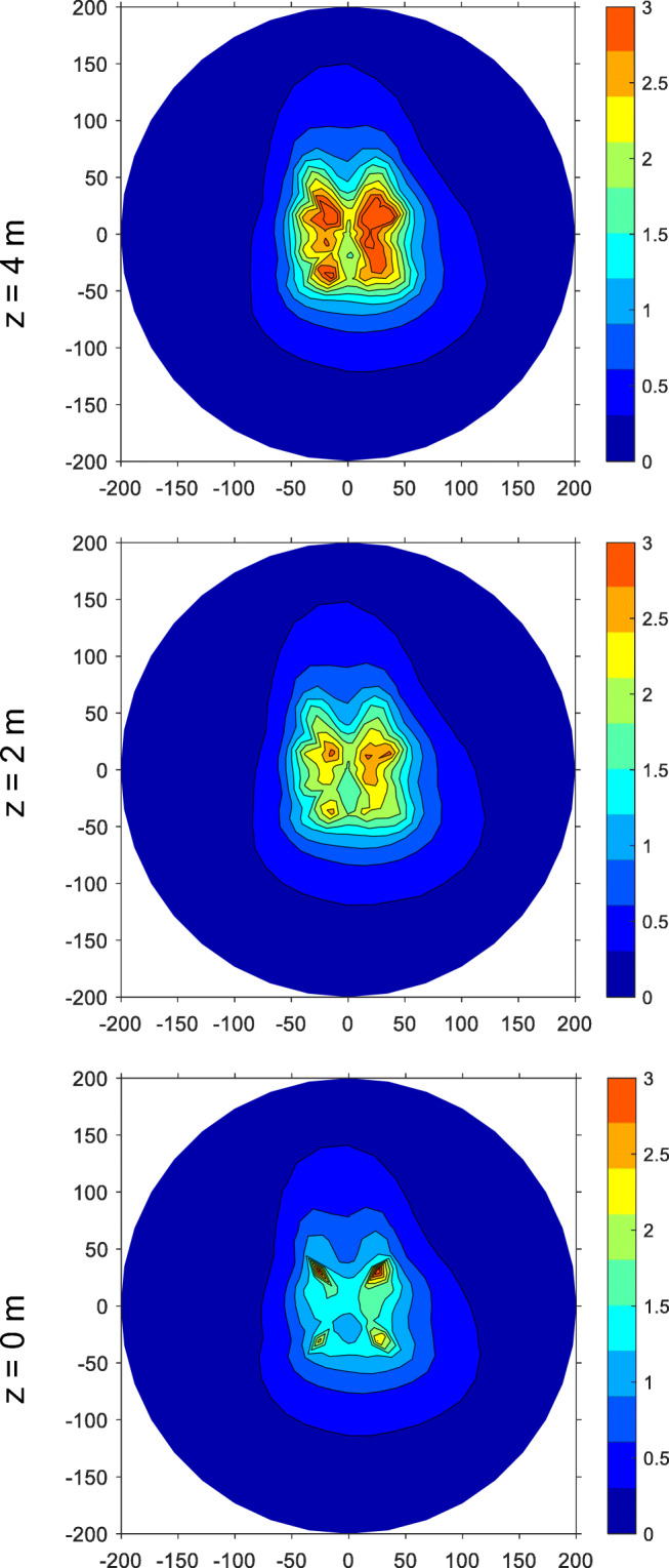
Modeled atmospheric benzene levels (3-year average) due to emissions from four-gas station configuration shown at 3 elevations: 0 (bottom panel), 2 (middle panel), and 4 m (top panel). Abscissa and ordinate labels indicate distance in meters. Color bar indicates benzene concentration in μg/m³

Close to the intersection (< 60 m), benzene levels depend substantially on elevation. At the 4-m elevation around the vent pipes, the only modeled point sources of benzene, concentrations tend to be highest. Further away from the intersection (>80 m), benzene levels do not depend much on elevation.

Figure 4 shows simulated atmospheric benzene levels in the breathing zone that arise from the four different gas stations clusters. Benzene levels clearly depend substantially on the number of gas stations present. Moreover, the spatially dependent concentration fields for more than one gas station cannot simply be obtained by multiplying the concentration field for one gas station by the number of gas stations in the cluster.

Fig. 4.

Modeled atmospheric benzene levels (3-year average) due to emissions from 4, 3, 2, and 1 gas station configuration at an elevation of 2 m. Abscissa and ordinate labels indicate distance in meters. Color bar indicates benzene concentration in μg/m³

Cancer risk modeling

Figure 5 shows boxplots of the log-transformed cancer risk normalized by total sales volume (left-hand-side of Eq. (2)) as a function of distance from the origin of the modeling domain. For distances ≥40 m, median normalized cancer risks are roughly the same for the four configurations. For distances <40 m (0 and 20 m), however, these risks differ substantially between configurations. Specifically, the single gas station exhibits different patterns, with cancer risk monotonically decreasing with distance; whereas for the configurations with more than one gas station cancer risk is greatest at a distance of 20 m. The heights of the box plots (interquartile range) in Fig. 5 also illustrate that cancer risk for a given distance and gas station configuration can vary by more than a factor of 10 depending on the angle φ_i.

Fig. 5.

Lifetime cancer risk <CR> normalized by total sales volume and then log-transformed for four different gas station clusters consisting of 1, 2, 3 and 4 gas stations by distance r from the origin of the model domain. Box plots indicate the variation of cancer risk at distance r due to its dependence on the angle φ_i at the z = 4 m elevation

Figure 6 shows the linear regressions for the log-transformed cancer risk medians, normalized by total sales volume, for the four different gas station configurations. Results from the regression analyses are summarized in Table 3. For all regressions, R² values are >0.96, and the F statistics are statistically significant (p < 0.05). In addition, all intercept and regression coefficients are statistically significant (p < 0.05), meaning distance and lifetime cancer risk are significantly associated. One-way ANOVA showed that regression coefficients a and b are not different across the four gas station configurations. At the same time, confidence intervals (CIs) between coefficients across gas station configurations overlapped. CIs of the regression coefficients that account for the data of all gas station configurations together overlap with the CIs from the four individual regressions.

Fig. 6.

Linear regression of the medians of lifetime cancer risk <CR> normalized by sales volume and then log-transformed for 1, 2, 3 and 4 gas stations. The regression excludes the first two distances (0 and 20 m)

Table 3.

Summary of linear regression for medians of lifetime cancer risk according to Eq. (2)

# Gas Stations	All	4	3	2	1
Intercept a [95% CI]	−5.50 [−5.55, −5.45]	−5.40 [−5.53, −5.28]	−5.42 [−5.53, −5.30]	−5.41 [−5.51, −5.32]	−5.45 [−5.61, −5.30]
Distance coefficient b (1/km)* [95% CI]	−6.49 [−6.91, −6.07]	−7.12 [−8.10, −6.15]	−7.04 [−7.92, −6.15]	−6.92 [−7.62, −6.22]	−7.03 [−8.19, −5.87]
R-squared	0.96	0.98	0.98	0.99	0.97
Cancer Risk at 40 m	N/A	9.84 × 10−6	6.94 × 10−6	4.66 × 10−6	2.45 × 10−6

*All intercepts and distance coefficients are statistically significant (p < 0.05)

Summary and discussion

Spatial dependence of benzene levels

We for the first time presented simulations for the cumulative effects of several gas stations on atmospheric benzene levels. As previously established, benzene levels depend substantially on distance from gas station [12–15, 25]; however, similar to Hilpert et al. [29], we also found that elevation is a determining factor [29]. Benzene levels on the ground surface (0-m elevation) and in the breathing zone (2-m elevation) are similar to each other (Fig. 3), because at lower elevations benzene levels arise from volume and surface forces and are not affected much by vent pipe emissions. Close to a gas station (< 40 m), benzene hot spots are present at a 4-m elevation where the vent pipes of the fuel storage tanks were assumed to release fuel vapors to the atmospheric environment, potentially putting residents at the 2nd floor level at risk. Further away from the center of the modeling domain (about >80 m), concentration fields do not depend much on elevation, as evidenced by the almost identical contour lines for benzene levels. This is because of vertical mixing of the benzene vapors due to atmospheric dispersion. Additionally, for quality assurance, we conducted a simulation for a single gas station where stack velocity is zero and compared the benzene concentration levels to our results (which use a stack velocity of 0.0012). We found that the percent difference for benzene concentration between the two simulations was close to zero.

Cancer risk as a function of sales volume and number of gas stations

We performed for the first time analyses that not only allow estimating cancer risk of a single gas station as a function of sales volume but also the risk from multiple gas stations in a cluster. In contrast, previous reports presented examples of cancer risk as a function of distance r only from a single gas station in the form of plots for a given sales volume SV, with no guidance about how to estimate cancer risk for a different sales volume. See, for example, Appendix E in CAPCOA [24] which presents cancer risks for gas stations dispensing 1 million gal/yr or Figs. 1, 2, 3, 4, 5 and 6 in CalEPA/CARB [26] for a gas station dispensing 3.6 million gal/yr [24, 26]. Our plots and Eq. (2), both of which normalize cancer risk by sales volume, respond to this need. For instance, one can now easily answer the question: what is the lifetime cancer risk <CR> of a single gas station dispensing 10 million gal/yr at a distance r = 150 m? We can read from the red line in Fig. 6, that log₁₀(…) ~ −6.5 and therefore . Since N_st = 1 and SV_single = 10⁷ gal/yr, the cancer risk is <CR> = 10^–5.5 which is 3 in a million.

Directional dependence of cancer risk

At a single location (specified by distance r and angle φ_i), substantial differences between the cancer risk inferred from Eq. (2) and the risk calculated from Eq. (1) using the AERMOD benzene concentration at that location may occur. This is because Eq. (2) represents a cancer risk averaged over all angles φ_i and because cancer risk may vary by more than an order of magnitude depending on φ_i for a given r (Fig. 5). Local meteorology and in particular variability in wind direction partially explain the spatial patterns and the directional dependence of modeled benzene concentrations, as a comparison between the wind rose (Supplemental Fig. 1) and the benzene concentrations fields (Figs. 3 and 4) shows. Therefore while Eq. (2) provides insights about how cancer risk depends on distance from gas station(s), detailed air dispersion simulations may be required to evaluate cancer risk for given receptor locations.

Equation for calculating cancer risk from gas station clusters

We proposed a simple equation, Eq. (2), which is based on an exponentially decaying function for estimating cancer risk as a function of distance from a gas station or a cluster of gas stations. Our statistical analysis (p-values and R²) showed that cancer risk is a function of distance from gas station(s). Based on a theoretical premise, modeled cancer risk could be expected to scale linearly with sales volume SV_single but it was not clear whether it would also scale linearly with the number of gas stations N_st. One-way ANOVA, however, supports the hypothesis that cancer risk (averaged over all angles φ_i) scales linearly with total sales volume SV_single N_st for distances ≥40 m as evidenced by the similarity of the normalized cancer risk plots for the four different gas station configurations (Fig. 5) and the regression analyses for Eq. (2). However, Eq. (2) should not be used outside the range of distances r used to inform the regression (40 to 200 m).

As an example for an application of Eq. (2), we use it to calculate cancer risk at a distance r = 150 m from the aforementioned gas station dispensing 10 million gal/yr. With a = −5.5 and b = −6.5 km⁻¹, log₁₀(…) = a + b r = −5.5 - 6.5 × 0.15 = −6.5, the same value determined from Fig. 6, thus also resulting in a cancer risk of 3 in a million.

Setback distances

Our Eq. (2), or variations thereof that account for actual emission rates and local meteorological conditions, provides a framework for formulating setback policies. E.g., if policy makers assume CR = 5 × 10⁻⁶ is an acceptable cancer risk, one can solve Eq. (2) for r to calculate the distance at which this cancer risk is obtained, e.g., for a cluster of N_st = 4 gas stations having each a sales volume SV_single = 3.6 million gal/year (or a single gas station dispensing 14.4 million gal/year): = 145 m. This distance can be interpreted as a setback distance, keeping in mind that cancer risk varies due to its directional dependence. This setback distance is much greater than the setback distance of 91 m recommended by CARB for California gas stations (with much lower emission factors) dispensing more than 3.6 million gal/year [26]. Thus, CARB guidelines should be used with caution if vapor emission control technology is below their standards.

Policy recommendations

While it is not surprising that cancer risks are higher for gas station clusters than for a single gas station, some policies on setback distances for gas stations account only for emissions from a single gas station [26], thereby neglecting the cumulative cancer risk arising from a cluster. We propose that policies should acknowledge the additional cancer risks arising from gas station clusters. This issue is of concern when a new gas station is built in an area where none is initially present and additional gas station(s) might be proposed thereafter or when a new gas station is built close to an existing one. Furthermore, our findings could provide a basis for improved standardization of policy at both the county and state level. Finally, we recommend that setback distances account for actual sales volume.

Limitations

Our study has some limitations. While we have devised an approach for estimating cancer risks from a gas station cluster, our study is not representative of any specific gas station development, because we only accounted for one set of meteorological conditions, assumed flat terrain, and made assumptions about fuel composition (benzene content) and emission prevention technology that are only representative of the US (except California). Indeed, according to an article published by the International Fuel Quality Center in 2009 benzene levels in gasoline can reach up to 7% in regions where these levels are regulated [39]; and levels can perhaps be even higher where not regulated. Moreover, benzene level may vary seasonally due to changes in fuel composition (winter versus summer fuel) [40–42] . However, because EPA [36] estimates of national gasoline benzene content (~ 1% by volume in 2016) and prior studies inform our assumptions, we feel they are a reasonable proxy. We also used emissions factors, which potentially underestimate actual emissions, as shown in a recent study that measured vent emissions at two fully functional US gas stations, finding that emissions greatly exceeded the emission factors listed in the CAPCOA (1997) study [24, 29].

Conclusions

We have developed a model to estimate cancer risk from gas station clusters, accounting for the increasing risk with additional gas stations and allowing for continuous rather than categorical sales volume inputs. Overall, we found that clusters of gas stations result in increased cancer risk compared to a single station. For instance, the cancer risk at 40 m for four gas stations each dispensing 1 million gal/year is 9.84 × 10⁻⁶ compared to 2.45 × 10⁻⁶ for one gas station. This framework can be utilized in real-life scenarios as a basis to estimate cancer risk by distance for gas station clusters in the US. Future work should consider developing a more general and widely applicable equation for cancer risk that also accounts for site-specific information such as emission factors, benzene content of the liquid gasoline and the gas phase in the ullage of the storage tank, and summary statistics of meteorological conditions. Future policies around setback distances should be reassessed to account for heightened risk from clusters.

Funding

MH was partially supported by National Institute of Environmental Health Sciences grant P30 ES009089, and JAS was supported by National Institute of Environmental Health Sciences grant T32 ES007322. The funding sources had no involvement in the study design; collection, analysis, and interpretation of data; report writing; or the decision to submit for publication.

Data availability

All data and material are publicly available.

Compliance with ethical standards

Conflicts of interest/Competing interests

The authors declare they have no conflict of interest.

Code availability

Code available upon request.

Ethics approval

This study does not involve human subjects.

References

- 1.U.S. Energy Information Administration (EIA), "U.S. Product Supplied of Finished Motor Gasoline," Washington, DC: U.S. Energy Infromation Administration, 2019. [Online]. Available: https://www.eia.gov/dnav/pet/hist/LeafHandler.ashx?n=pet&s=mgfupus1&f=m.
- 2.Census. U.S., World Population Clock. United States Census Bureau, U.S. Department of Commerce. 2009.
- 3.Hilpert M, Breysse PN. Infiltration and evaporation of small hydrocarbon spills at gas stations. J Contam Hydrol. 2014;170:39–52. doi: 10.1016/j.jconhyd.2014.08.004. [DOI] [PubMed] [Google Scholar]
- 4.Hilpert M, Mora BA, Ni J, Rule AM, Nachman KE. Hydrocarbon Release During Fuel Storage and Transfer at Gas Stations: Environmental and Health Effects. Curr Environ Health Rep. 2015;2(4):412–422. doi: 10.1007/s40572-015-0074-8. [DOI] [PubMed] [Google Scholar]
- 5.Mora BA, Hilpert M. Differences in Infiltration and Evaporation of Diesel and Gasoline Droplets Spilled onto Concrete Pavement, Sustainability (Switzerland). 2017; 9: 10.3390/su9071271.
- 6.Morgester JJ, Fricker RL, Jordan GH. Comparison of Spill Frequencies and Amounts at Vapor Recovery and Conventional Service Stations in California. J Air Waste Manage Assoc. 1992;42(3):284–289. doi: 10.1080/10473289.1992.10466991. [DOI] [Google Scholar]
- 7.Agency for Toxic Substances and Disease Registry (ATSDR), "Interaction profile for benzene, toluene, ethylbenzene, and xylenes (BTEX)," Atlanta, GA: U.S. Department of Health and Human Services, Public Health Service, 2004. [PubMed]
- 8.Crossin R, Lawrence AJ, Andrews ZB, Churilov L, Duncan JR. Growth changes after inhalant abuse and toluene exposure: a systematic review and meta-analysis of human and animal studies. Hum Exp Toxicol. 2019;38(2):157–172. doi: 10.1177/0960327118792064. [DOI] [PubMed] [Google Scholar]
- 9.Varjani SJ, Gnansounou E, Pandey A. Comprehensive review on toxicity of persistent organic pollutants from petroleum refinery waste and their degradation by microorganisms. Chemosphere. 2017;188:280–291. doi: 10.1016/j.chemosphere.2017.09.005. [DOI] [PubMed] [Google Scholar]
- 10.IARC. International Agency for Research on Cancer (IARC) monographs on the evaluation of carcinogenic risks to humans. vol. 100F, 2012. [Online]. Available: http://monographs.iarc.fr/ENG/Monographs/vol100F/.
- 11.Lan Q, et al. Hematotoxicity in workers exposed to low levels of benzene. Science (New York, NY) 2004;306(5702):1774–1776. doi: 10.1126/science.1102443. [DOI] [PMC free article] [PubMed] [Google Scholar]
- 12.Morales Terrés IM, Miñarro MD, Ferradas EG, Caracena AB, Rico JB. Assessing the impact of petrol stations on their immediate surroundings. J Environ Manag. 2010;91(12):2754–2762. doi: 10.1016/j.jenvman.2010.08.009. [DOI] [PubMed] [Google Scholar]
- 13.Jo WK, Oh JW. Exposure to methyl tertiary butyl ether and benzene in close proximity to service stations. J Air Waste Manag Assoc (1995) 2001;51(8):1122–8. doi: 10.1080/10473289.2001.10464339. [DOI] [PubMed] [Google Scholar]
- 14.Jo W-K, Moon K-C. Housewives’ exposure to volatile organic compounds relative to proximity to roadside service stations. Atmos Environ. 1999;33(18):2921–2928. doi: 10.1016/S1352-2310(99)00097-7. [DOI] [Google Scholar]
- 15.Correa SM, Arbilla G, Marques MRC, Oliveira KMPG. The impact of BTEX emissions from gas stations into the atmosphere. Atmospher Pollut Res. 2012;3(2):163–169. doi: 10.5094/APR.2012.016. [DOI] [Google Scholar]
- 16.Hajizadeh Y, et al. Trends of BTEX in the central urban area of Iran: A preliminary study of photochemical ozone pollution and health risk assessment. Atmospher Pollut Res. 2018;9(2):220–229. doi: 10.1016/j.apr.2017.09.005. [DOI] [Google Scholar]
- 17.Hicklin W, Farrugia PS, Sinagra E. Investigations of VOCs in and around buildings close to service stations. Atmos Environ. 2018;172:93–101. doi: 10.1016/j.atmosenv.2017.10.012. [DOI] [Google Scholar]
- 18.Barros N, et al. Environmental and biological monitoring of benzene, toluene, ethylbenzene and xylene (BTEX) exposure in residents living near gas stations. J Toxic Environ Health A. 2019;82(9):550–563. doi: 10.1080/15287394.2019.1634380. [DOI] [PubMed] [Google Scholar]
- 19.Infante PF. Residential proximity to gasoline stations and risk of childhood leukemia. Am J Epidemiol. 2017;185(1):1–4. doi: 10.1093/aje/kww130. [DOI] [PMC free article] [PubMed] [Google Scholar]
- 20.Steffen C, Auclerc MF, Auvrignon A, Baruchel A, Kebaili K, Lambilliotte A, Leverger G, Sommelet D, Vilmer E, Hémon D, Clavel J. Acute childhood leukaemia and environmental exposure to potential sources of benzene and other hydrocarbons; a case-control study. Occup Environ Med. 2004;61(9):773–778. doi: 10.1136/oem.2003.010868. [DOI] [PMC free article] [PubMed] [Google Scholar]
- 21.Brosselin P, et al. Acute childhood leukaemia and residence next to petrol stations and automotive repair garages: the ESCALE study (SFCE). Occup Environ Med. 2009;66(9):598–606. 10.1136/oem.2008.042432. [DOI] [PubMed]
- 22.Harrison RM, Leung PL, Somervaille L, Smith R, Gilman E. Analysis of incidence of childhood cancer in the west midlands of the United Kingdom in relation to proximity to main roads and petrol stations. Occup Environ Med. 1999;56(11):774–780. doi: 10.1136/oem.56.11.774. [DOI] [PMC free article] [PubMed] [Google Scholar]
- 23.Baghani AN, et al. A case study of BTEX characteristics and health effects by major point sources of pollution during winter in Iran. Environ Pollut (Barking, Essex : 1987) 2019;247:607–617. doi: 10.1016/j.envpol.2019.01.070. [DOI] [PubMed] [Google Scholar]
- 24.California Air Pollution Control Officers Association (CAPCOA), "Gasoline Service Station Industrywide Risk Assessment Guidelines," Toxics Committee of the California Air Pollution Control Officers Association (CAPCOA), 1997.
- 25.Wu B-Z, Hsieh L-L, Chiu K-H, Sree U, Lo J-G. Determination and impact of volatile organics emitted during rush hours in the ambient air around gasoline stations. J Air Waste Manage Assoc. 2006;56(9):1342–1348. doi: 10.1080/10473289.2006.10464589. [DOI] [PubMed] [Google Scholar]
- 26.CalEPA. Air quality and land use handbook: a community health perspective. California Environmental Protection Agency & California Air Resources Board. 2005.
- 27.Mohai P, Kweon B-S. Michigan school siting guidelines: taking the environment into account. University of Michigan. 2020. [Online]. Available: https://deepblue.lib.umich.edu/handle/2027.42/156009.
- 28.Montgomery. Zoning text amendments: filling station - use standards ZTA-15-07. Montgomery County Council. 2015. [Online]. Available: https://www.montgomerycountymd.gov/COUNCIL/Resources/Files/zta/2015/20151201_18-07.pdf.
- 29.Hilpert M, Rule AM, Adria-Mora B, Tiberi T. Vent pipe emissions from storage tanks at gas stations: Implications for setback distances. Sci Total Environ. 2019;650:2239–2250. doi: 10.1016/j.scitotenv.2018.09.303. [DOI] [PMC free article] [PubMed] [Google Scholar]
- 30.NOAA/ESRL. NOAA/ESRL Radiosonde Database. [Online]. Available: https://ruc.noaa.gov/raobs/. Accessed 3 Nov 2018
- 31.EPA. User's Guide for the AMS/EPA Regulatory Model (AERMOD). vol. EPA-454/B-19-027, 2019.
- 32.EPA. User’s Guide for the AERMOD Meteorological Preprocessor (AERMET). vol. EPA-454/B-19-028, 2019.
- 33.Cimorelli AJ, Perry SG, Venkatram A, Weil JC, Paine RJ, Wilson RB, Lee RF, Peters WD , Brode RW, Paumier JO. AERMOD: description of model formulation. U.S. Environmental Protection Agency, Office of Air Quality Planning and Standards, Emissions Monitoring and Analysis Division, vol. EPA-454/R-03-004, 2004. [Online]. Available: https://www3.epa.gov/scram001/7thconf/aermod/aermod_mfd.pdf.
- 34.Perry SG, et al. AERMOD: A Dispersion Model for Industrial Source Applications. Part II: Model Performance against 17 Field Study Databases. J Appl Meteorol. 2005;44(5):694–708. doi: 10.1175/JAM2228.1. [DOI] [Google Scholar]
- 35.Environmental Protection Agency (EPA), "Air Quality: Widespread Use for Onboard Refueling Vapor Recovery and Stage II Waiver. 2012; 77: 95.
- 36.EPA. Gasoline mobile source air toxics. U.S. Environmental Protection Agency. https://www.epa.gov/gasoline-standards/gasoline-mobile-source-air-toxics (accessed.).
- 37.EPA. Risk assessment guidance for superfund volume I: human health evaluation manual (Part F, Supplemental Guidance for Inhalation Risk Assessment. vol. EPA-540-R-070-002, 2009.
- 38.Seinfeld JH, Pandis SN. Atmospheric chemistry and physics: from air pollution to climate change. Hoboken: Wiley; 2016. [Google Scholar]
- 39.Poirier L, Vora K.. Top-100 Countries Ranked by. Standards for gasoline benzene limits al fuel.. Hart Energy Consulting, 2009. [Online]. Available: http://environmentportal.in/files/Gasoline%20benzene%20limits.pdf.
- 40.Gentner DR, Harley RA, Miller AM, Goldstein AH. Diurnal and Seasonal Variability of Gasoline-Related Volatile Organic Compound Emissions in Riverside, California. Environ Sci Technol. 2009;43(12):4247–4252. doi: 10.1021/es9006228. [DOI] [PubMed] [Google Scholar]
- 41.Zimmerman N, et al. Field Measurements of Gasoline Direct Injection Emission Factors: Spatial and Seasonal Variability. Environ Sci Technol. 2016;50(4):2035–2043. doi: 10.1021/acs.est.5b04444. [DOI] [PubMed] [Google Scholar]
- 42.Chin J-Y, Batterman SA. VOC composition of current motor vehicle fuels and vapors, and collinearity analyses for receptor modeling. Chemosphere. 2012;86(9):951–958. doi: 10.1016/j.chemosphere.2011.11.017. [DOI] [PMC free article] [PubMed] [Google Scholar]
Associated Data
This section collects any data citations, data availability statements, or supplementary materials included in this article.
Supplementary Materials
(DOCX 55 kb)
Data Availability Statement