Abstract
High-dimensional variable selection in the proportional hazards (PH) model has many successful applications in different areas. In practice, data may involve confounding variables that do not satisfy the PH assumption, in which case the stratified proportional hazards (SPH) model can be adopted to control the confounding effects by stratification without directly modeling the confounding effects. However, there is a lack of computationally efficient statistical software for high-dimensional variable selection in the SPH model. In this work an R package, SurvBoost, is developed to implement the gradient boosting algorithm for fitting the SPH model with high-dimensional covariate variables. Simulation studies demonstrate that in many scenarios SurvBoost can achieve better selection accuracy and reduce computational time substantially compared to the existing R package that implements boosting algorithms without stratification. The proposed R package is also illustrated by an analysis of gene expression data with survival outcome in The Cancer Genome Atlas study. In addition, a detailed hands-on tutorial for SurvBoost is provided.
Introduction
Variable selection for high-dimensional survival data has become increasingly important in a variety of research areas. One of the most popular methods is based on the proportional hazards (PH) model. Many penalized regression methods including adaptive lasso and elastic net have been proposed for the PH model (Tibshirani, 1997; Simon et al., 2011; Goeman, 2010). Alternatively, boosting described by Bühlmann and Yu (2010) has been adopted for variable selection in regression models and the PH model via gradient descent techniques. It can have a better variable selection accuracy compared with other methods in many scenarios. The R package mboost has been developed and become a powerful tool for variable selection and parameter estimation in complex parametric and nonparametric models via the boosting methods (Hothorn et al., 2017). It has been widely used in many applications.
However, in many biomedical studies, the collected data may involve confounding variables that do not satisfy the PH assumption. For example, in cancer research you may argue that gender effects are not proportional, but we are more interested in selecting genes as the important risk factors for cancer survival. The PH assumption can reasonably be imposed on modeling the gene effects but not for gender effects. In this case the stratified proportional hazards (SPH) models are needed. In particular, the data are often grouped into multiple strata according to confounding variables. The SPH model adjusts those confounding effects by fitting the Cox regression with different baseline hazards for different strata, while still assuming that the covariate effects of interest are the same across different strata and satisfy the proportional hazard assumption.
The SPH model has a wide range of applications for survival analysis, but no computationally efficient statistical software are available for high-dimensional variable selection in the SPH model. To fill this gap, we develop an R package, SurvBoost, to implement the gradient boosting algorithm for fitting the SPH model with high-dimensional covariates with adjusting confounding variables. SurvBoost implements the gradient descent algorithm for fitting both PH and SPH model. The algorithm for the PH model has been used for the additive Cox model in the mboost package, which cannot fit the SPH model to perform variable selection. The survival package is capable of performing model fitting for the SPH model, but does not implement variable selection desired in the high-dimensional setting. In our SurvBoost package, we optimize the implementations which can reduce 30%–50% computational time. Additional options are available in the SurvBoost package to determine an appropriate stopping criteria for the algorithm. Another useful function assists in selecting stratification variables, which may improve model fitting results.
The rest of the paper is organized as follows: In Section 2, we will provide a brief overview of the gradient boosting method for the SPH model along with the algorithm stopping criteria. In Section 3, we show that SurvBoost can achieve a better selection accuracy and reduce computational time substantially compared with mboost. In Section 4, we provide a detailed hands-on tutorial for SurvBoost. In Section 5, we illustrate the proposed R package on an analysis of the gene expression data with survival outcome in The Cancer Genome Atlas (TCGA) study.
Methods
Stratified proportional hazards model
The Cox proportional hazards model is effective for modeling survival outcomes in many applications. An important assumption underlying this model is a constant hazard ratio, meaning that the hazard for one individual is proportional to that of any other individual. This is a strong assumption for many applications. Thus, one useful adaptation to this model is relaxing the strict proportional hazards assumption; one approach is to allow the baseline hazard to differ by group across the observations. This is known as the stratified proportional hazards (SPH) model.
Suppose the dataset consists of n subjects. For i = 1, … , n, denote by Ti the observed time of event or censoring for subject i, and δi indicates whether or not an event occurred for subject i. Denote by G the total number of strata and by ng the number of subjects in stratum g. Let gi be the strata indicator for subject i. Suppose there are p potential covariate variables of our interest to select. For j = 1, … , p, let xij be the covariate j for subject i. For stratum g = 1, … , G, the hazard of subject i at time t in stratum g becomes
where h0,g(t) is the baseline hazard function, Xi,g is a vector of covariates and β is the regression coefficients of interest.
Allowing the baseline hazard to differ across strata allows flexibility often desired when proportional hazards is too strong. The SPH model can control effects of confounding variables through this stratification. The estimates of the effect of covariates remain constant across strata, so the model is still interpretable across all subjects.
Gradient boosting for SPH
The log partial likelihood of the SPH model is
where β = (β1, … , βp)⊤, Xi = (Xi1, … , Xip)⊤ and Rig = {ℓ : Tℓ ≥ Ti,gl = g} for all i with gi = g representing the set of at risk subjects in group g. We adopt the following gradient boosting algorithm to find the maximum partial likelihood estimate (MPLE). Let for k = 0,1,2.
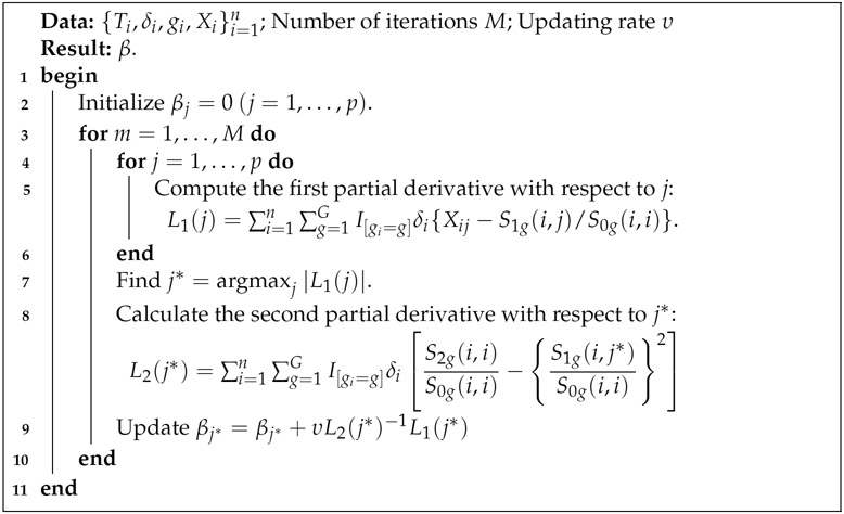
Algorithm 1:
Boosting gradient descent algorithm
This algorithm updates variables one at a time, by selecting the variable which maximizes the first partial derivative. The number of iterations is important for ensuring a sufficient number of updates to the β estimates, in addition to selecting the true signals (He et al., 2016). Note that this algorithm is slightly different than the one implemented in the mboost package even in the unstratified case, which we will use for comparison in the simulation setting. Buhlmann and Hothorn’s algorithm uses only the first derivative to update the estimated β values (Bühlmann and Hothorn, 2007).
Stopping criteria
Selection of the number of boosting iterations is important. Over-fitting can occur if the number of iterations is too large (Jiang, 2004). Additionally the stopping criteria is important for accuracy of the coefficient estimates, since each iteration contributes to updating the estimate of one coefficient. The algorithm is less sensitive to the step size (Bühlmann and Hothorn, 2007).
SurvBoost provides several options for optimizing the number of iterations including: k-fold cross validation, Bayesian information criteria, change in likelihood, or specifying the number of variables to select.
The Bayesian Information Criteria (BIC) is one approach for selecting the optimal number of boosting iterations.
| (1) |
where is the maximized likelihood for a model with pj selected variables and is the maximized likelihood for the reference model with p0 selected variables. The number of uncensored events is d. Volinsky and Raftery (2000) argue that replacing the sample size, n, with d in the BIC calculation has better properties when dealing with censored survival models.
The extended BIC is also useful in high dimensional cases; this approach penalizes for greater complexity
| (2) |
where is the size of the class of models that model j belongs to, p is the total number of variables. The value of γ is fixed between 0 and 1, selected to penalize at the appropriate rate. Selecting 0 will reduce this to the standard BIC; EBIC and BIC are implemented jointly in the package using this connection to reduce from EBIC to BIC. AIC is available as well as a stopping criteria, although this information might not be as effective in the high dimensional setting.
Cross validation is another approach which may be used to determine the stopping point. The goodness of fit function is calculated as suggested by Simon et al. (2011). It is the log-partial likelihood of all the data using the optimal β determined with data excluding fold k(β−k) minus the log-partial likelihood excluding fold k(ℓ−k) of the data with the same β.
| (3) |
Where m is the current number of iterations and k indicates the subset of data being excluded.
Change in likelihood is another approach incorporated in the package. This method stops iterating once a small change in likelihood, specified in the function, is reached.
| (4) |
Where α is a small constant. Default change in likelihood, used in simulations, is a change of 0.001.
Simulation studies
This section compares the variable selection performance to a competing R package, mboost (Hofner et al., 2014).
Stratified Data
Stratified data was simulated such that censoring rates were relatively constant across groups and the expected survival time differed by group. These assumptions mimic realistic settings such as those encountered with data grouped by hospital or facility.
For this simulation 1,500 observations were generated into ten strata; each strata had a different baseline hazard following a Weibull distribution. The Weibull distribution shape parameter was 3 for all strata, and the scale parameter varied across strata from e−1 to e−15 with ten evenly spaced intervals. There were 100 true signals among 4,000 variables with true magnitude of 2 or −2. There was uniform censoring from time 0 to 200. Fifty of these data sets were generated.
The following example demonstrates the importance of the stopping criteria. SurvBoost has five options for specifying the number of iterations as described in the methods section. Selecting an appropriate number of iterations depends on the goals of the analysis. For example, if the goal is to achieve high sensitivity cross validation or extended BIC may be the best approach.
The performance of different stopping criteria are compared based on several selection and estimation measures: sensitivity (Se), specificity (Sp), false discovery rate (FDR), and mean squared error (MSE). FDR is calculated as the ratio of false positives over the total number of selected variables. Sensitivity, specificity, and FDR aim to address the performance of the variable selection, while MSE aims to address the accuracy of the coefficient estimates.
This simulation presents the performance of SurvBoost compared to the R package mboost. The boosting algorithm implemented in mboost is very similar to that of SurvBoost but does not allow stratification. We will compare results between the two packages using only a fixed number of iterations as the stopping rule; mboost has K-fold cross validation available for some settings but no longer provides it for Cox PH models. All of the stopping methods implemented in SurvBoost are not available in mboost. The performance can be compared by measures such as sensitivity and mean squared error. Table 1 presents the results of 50 simulated data sets, comparing the boosting algorithm using several different stopping procedures and to results from mboost. In this simulation, mboost selects fewer variables on average resulting in fewer false positives and more false negatives. Additionally the mean squared error is slightly higher than that of all the SurvBoost options.
Table 1:
Results from simulation with approximately 1,500 observations in 10 strata and 4,000 variables to be selected. The table presents averages with the standard deviation, in parentheses, from 50 simulated datasets. Sensitivity (Se) is calculated as the proportion of true positives out of the total number of true signals. Specificity (Sp) is calculated as the proportion of true negatives out of the total number of variables that are not true signals. The false discovery rate (FDR) is the proportion of false positives in the total number of selected variables.
| stopping method |
number selected |
Se | Sp | FDR | MSE | number of iterations |
runtime (seconds) |
|
|---|---|---|---|---|---|---|---|---|
| SurvBoost | fixed | 111 (5) | 0.90 (.02) | 0.99 (.00) | 0.19 (.04) | 382 (1) | 500 (0) | 163 (20) |
| mboost | 99 (4) | 0.82 (.03) | 1.00 (.00) | 0.17 (.04) | 387 (1) | 500 (0) | 396 (254) | |
| SurvBoost | cv | 379 (24) | 1.00 (.00) | 0.93 (.01) | 0.74 (.02) | 333 (3) | 3896 (275) | 5742 (595) |
| SurvBoost | # selected | 101 (0) | 0.84 (.03) | 1.00 (.00) | 0.17 (.03) | 385 (2) | 385 (40) | 163 (24) |
| SurvBoost | likelihood | 121 (6) | 0.95 (.02) | 0.99 (.00) | 0.21 (.04) | 378 (1) | 632 (15) | 242 (33) |
| SurvBoost | EBIC | 140 (7) | 0.99 (.01) | 0.99 (.00) | 0.29 (.04) | 370 (1) | 993 (10) | 624 (60) |
Runtime is also an important factor with this algorithm. Stratification speeds up the algorithm as seen in the first simulation. All runtimes were generated on a MacBook with 2.9GHz Intel Core i5 and 16GB memory.
To further demonstrate the importance of using the SPH model, we compared results of modeling with and without stratification for data simulated with ten strata. In this setting the true signal for all 100 variables is 0.75 to illustrate the performance with a smaller effect size.
From this example we can evaluate the importance of using the stratified model. This case demonstrates that when not stratifying by group the model is not as sensitive to the true signals, resulting in lower sensitivity. We also observe a larger or similar number of variables selected, meaning that there are a larger number of false positives when ignoring the stratification. Depending on the context, a larger number of false positives may be very undesirable. The algorithm implemented for the Cox PH model is slightly different than the one used in SurvBoost, which can be seen here by the difference in the two unstratified rows.
Unstratified Data
Another simulation was used to compare performance of our method to mboost when stratification is not necessary for appropriate modeling. Similarly to the stratified case, four thousand variables were generated for 1,500 observations but without stratification. The baseline hazard followed a Weibull distribution, with shape parameter equal to 5 and scale equal to exp−5. The true β contained 100 true signals of magnitude 2 or −2 out of 4,000 variables.
We can observe in Table 2 that SurvBoost performs similarly to mboost under these conditions. mboost tends to select fewer variables than SurvBoost, so in this simulation mboost has fewer false positives and more false negatives compared to SurvBoost.
Table 2:
Results from simulation with approximately 1,000 observations and 1,000 possible variables for selection with 100 true signals. The table presents averages with the standard deviation from 50 simulated datasets. All methods in this table were run using the SurvBoost package except for the unstratified mboost row.
| Stopping Method |
number selected |
Se | Sp | FDR | MSE | number of iterations |
runtime (seconds) |
|
|---|---|---|---|---|---|---|---|---|
| Stratified | fixed | 116 (7) | 0.71 (.04) | 0.95 (.01) | 0.39 (.04) | 49 (0) | 500 (0) | 14 (1) |
| cv | 198 (16) | 0.90 (.04) | 0.88 (.02) | 0.54 (.03) | 50 (2) | 1585 (316) | 263 (60) | |
| # selected | 100 (0) | 0.65 (.04) | 0.96 (.00) | 0.36 (.04) | 50 (1) | 391 (42) | 11 (2) | |
| likelihood | 112 (8) | 0.69 (.04) | 0.95 (.01) | 0.38 (.03) | 49 (1) | 472 (33) | 14 (2) | |
| EBIC | 161 (9) | 0.84 (.03) | 0.91 (.01) | 0.48 (.04) | 44 (1) | 41 (45) | 29 (3) | |
| Unstratified | SB fixed | 122 (7) | 0.67 (.04) | 0.94 (.01) | 0.45 (.04) | 49 (1) | 500 (0) | 13 (1) |
| mboost | 58 (5) | 0.41 (.03) | 0.98 (.00) | 0.30 (.06) | 53 (0) | 500 (0) | 13 (1) |
Illustration of package
This section provides a brief tutorial on how to use this package based on simulated data. In order to install the package, several other R packages must be installed. The code relies on Rcpp, RcppArmadillo, and RcppParallel in order to improve computational speed (Eddelbuettel et al., 2018a,b; Allaire et al., 2018). Additionally the survival package is used for simulation and post selection refitting for inference and will be required for installation of SurvBoost (Therneau, 2017). If working on a Windows machine, installing Rtools is also necessary. The following line of R code installs the package from CRAN.
R > install.packages(“SurvBoost”)
Model fitting
The boosting_core() function requires similar inputs to the familiar coxph() function from the package survival.
boosting_core(formula, data = matrix(), rate = 0.01, num_iter = 500, …)
The input formula has the form Surv(time,death) ~ variable1 + variable2. The input data is in matrix form or a data frame. Two additional parameters must be specified for the boosting algorithm: rate and num_iter. Rate is the step size in the algorithm, although choice of this may not impact the performance too significantly (Bühlmann and Hothorn, 2007), default value is set to 0.01. Selecting an appropriate number of iterations to run the algorithm will, however, have a greater impact on the results. The last input num_iter is used to determine the number of iterations to run the algorithm, default value is 500.
Simple example
We present a simple example demonstrating the convenience of using the package for stratified data. We simulate survival data for five strata with different constant baseline hazards.
R > TrueBeta
 [1] 0.5 0.5 0.0 0.0 0.0 −0.5 0.5 0.5 0.0 0.0
R > set.seed(123)
R >  data_small <- simulate_survival_cox(true_beta=TrueBeta,
               base_hazard=“auto”,
               num_strata=5,
               input_strata_size=100, cov_structure=“ar”,
               block_size=5, rho=0.6, censor_dist=“unif”,
               censor_const=2, tau=Inf, normalized=F)
We have p = 10 and ∣βj∣ ranges from 0 to 0.5. There are five “facilities” with average size of 100 each representing one stratum, and n is approximately 500. The covariance structure within the blocks is AR(1) with correlation 0.6. The censoring rate is about 33%. In this case the variable strata_idx indicates the variable to stratify on in the survival model; each “facility” in this simulated data has a different baseline hazard function.
Another feature of the package assists with determining variables to stratify on if this information is unknown. The function strata.boosting will print box plots and a summary table of the survival time grouped by splits in the specified variable. The variable can be categorical or continuous; if continuous, the function will split on the median value to demonstrate whether there appears to be a difference in the survival time distribution for the two groups. This information alone does not suggest that stratification on this variable is necessary. It is intended to be a tool to confirm if there are differences seen across groups, when stratification is anticipated to be necessary.
R > strata.boosting(data_small$strata_idx, data_small$time)

  as.factor(x)          Min        Q1    Median      Q3       Max
1            1 0.0046772744 0.1163388 0.3108169 1.096236 1.693283
2            2 0.0005600448 0.1422992 0.5849665 1.270754 1.951286
3            3 0.0057943145 0.1371938 0.9125127 1.314191 1.989180
4            4 0.0042511208 0.1998902 0.5797646 1.437124 1.960646
5            5 0.0015349222 0.1283325 0.5896426 1.325094 1.873137
Simulated data includes a vector of survival or censoring time, time, indicator of an event, delta, and matrix of covariates, Z. Then generate the formula including all possible variables for selection.
R > time <- data_small$time
R > delta <- data_small$delta
R > Z <- as.matrix(data_small[,-c(1,2,3)])

R > covariates <- paste(“strata(strata_idx)+”, paste(colnames(Z),
    collapse = “+”))
R > formula <- as.formula(paste(“Surv(time,delta)~”, covariates))
Run the boosting_core() function to obtain the variables selected. This example uses the number of iterations control as a fixed input of 75 and update rate of 0.1.
R > test1 <- boosting_core(formula,
+              data=data_small,
+              rate=0.1,
+              num_iter=75)
R > summary.boosting(test1)

Call:
boosting_core(formula = formula, data = data_small, rate = 0.1,
    num_iter = 75)

 data: data_small

 n = 506
 Number of events = 371
 Number of boosting iterations: mstop = 75
 Step size = 0.1

 Coefficients:
        V1         V2         V6         V7         V8
 0.4486589  0.3676104 −0.2150421  0.2384806  0.4728502
Function summary.boosting() displays the variables which are selected as well as the coefficient estimates and the number of boosting iterations performed. Set the argument all_beta = TRUE to see all the variables, not just those selected.
To use a different method for the number of boosting iterations use the arguments control_method and control_parameter. The value of control_parameter should be a list containing the value of the parameter(s) corresponding to the method specified by control_method. For example,
R > test2 <- boosting_core(formula, data=data_small, rate=0.1,
           control_method=“num_selected”, control_parameter=list(num_select=5))
R > summary.boosting(test2)
Call:
boosting_core(formula = formula, data = data_small, rate = 0.1,
    control_method = “num_selected”, control_parameter = list(num_select = 5))

 data: data_small

 n = 506
 Number of events = 371
 Number of boosting iterations: mstop = 104
 Step size = 0.1

Coefficients:
        V1         V2         V6         V7         V8
0.11828718 0.11021464 −0.05292158 0.25561965 0.05199151

 Number of iterations:  10
This option iterates until the specified number of variables, 5 in this example, are selected. See methods for other stopping criteria. Note that in the package BIC and EBIC are available jointly in one option when control_method is set to "BIC". Setting the parameter γ = 0 will reduce the EBIC penalty to the BIC penalty. In order to implement EBIC, a nonzero value of gamma should be specified in control_parameter.
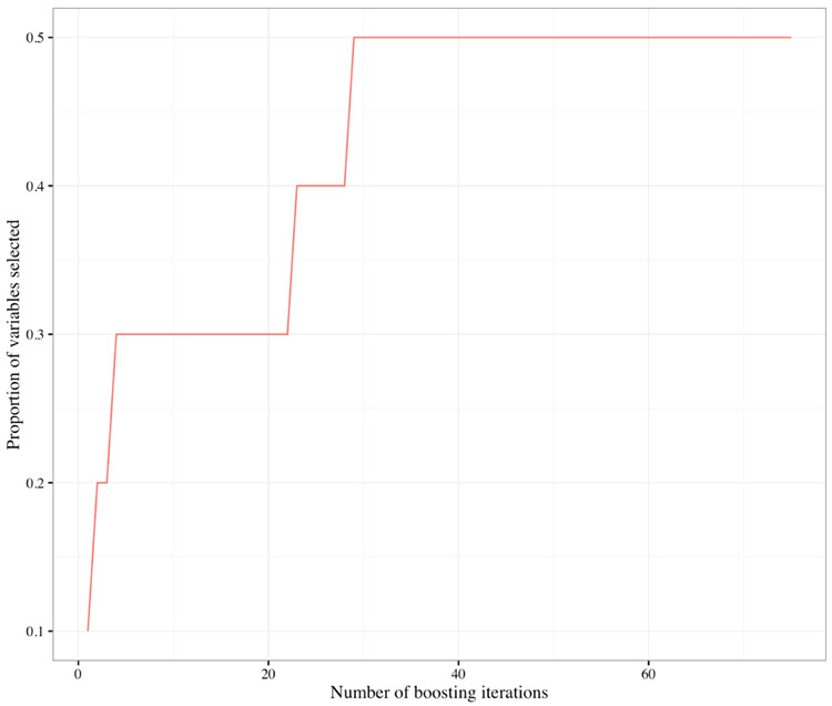
The plot.boosting() function displays a plot of the selection frequency by the number of iterations. Another option of the plot.boosting() function is to plot the coefficient paths of each variable by the number of boosting iterations. See Figures 2 and 3.
Figure 2:
Plot generated by plot.boosting function, variable selection frequency by number of boosting iterations.
Figure 3:
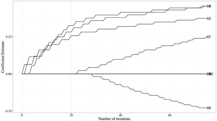
Plot generated by plot.boosting function with option “coefficients,” coefficient paths for variables selected by number of boosting iterations.
The function predict.boosting() provides an estimate of the hazard ratio for each observation in the dataset provided, relative to the average of p predictors.
R > predict.boosting(test1)[1:6]
46.385476 1.823920 42.049932 16.427860 4.013200 2.243711
The model selected using boosting can be refit with coxph() for post selection inference. The function post.selection.fitting.boosting() will perform this refitting and output the coefficient estimates with corresponding standard errors and p-values. Note that the statistical inferences performed here are conditional on the variable selection results. The interpretation of p-values and standard errors are fundamentally different from the regular unconditional statistical inferences. The performance of conditional statistical inferences is highly dependent on the variable selection accuracy. In our case, it depends on the choice of stopping rule.
R > summary.test1 <- summary.boosting(test1)
R > fmla <- summary.test1$formula
R > post.selection.fitting.boosting(fmla, data=data_small)
Call:
coxph(formula = fmla, data = data)

  n = 506, number of events = 371

       coef exp(coef) se(coef)      z Pr(>∣z∣)
V1  0.59181   1.80726  0.07454  7.940 2.00e-15 ***
V2  0.48079   1.61736  0.06948  6.920 4.53e-12 ***
V6 −0.51830   0.59553  0.07145 −7.254 4.05e-13 ***
V7  0.51108   1.66709  0.08479  6.028 1.66e-09 ***
V8  0.54758   1.72907  0.07116  7.695 1.42e-14 ***
---
Signif. codes: 0 '***' 0.001 '**' 0.01 '*' 0.05 '*' 0.1 ' ' 1

   exp(coef) exp(-coef) lower .95 upper .95
V1    1.8073     0.5533    1.5616    2.0915
V2    1.6174     0.6183    1.4114    1.8533
V6    0.5955     1.6792    0.5177    0.6851
V7    1.6671     0.5998    1.4118    1.9685
V8    1.7291     0.5783    1.5040    1.9879

Concordance= 0.762  (se = 0.036 )
Rsquare= 0.487   (max possible= 0.997 )
Likelihood ratio test= 338.1 on 5 df,   p=0
Wald test            =287.8 on 5 df,    p=0
Score (logrank) test = 299.1 on 5 df,   p=0
TCGA data example
Data from three breast cancer cohorts was used to demonstrate this method on data outside of the simulation framework. There were 578 patients included in the combined data, with 8,864 variables measured for each patient: 8,859 genes and 5 phenotypic variables. The phenotype variables included age at diagnosis, tumor size, cancer stage, progesterone-receptor status, and estrogen-receptor status. The data can be downloaded from The Cancer Genome Atlas (TCGA) (Naderi et al., 2006; Chin et al., 2006; Miller et al., 2005) or from GitHub using the following R code.
R > library(piggyback)
R > pb_download(“data.tcga.tsv.gz”,
            repo = “EmilyLMorris/survBoost”)
R > data <- read_tsv(“data.tcga.tsv”)
The patients were split into two cohorts depending on their cancer stage and tumor size. One cohort contained patients with a less severe prognosis, cancer stage of one and tumor size less than the median; the other cohort contained those with cancer stage greater than one and/or with a tumor larger than the median size.
R > fit.plot <- survfit(Surv(survival_time, survival_ind) ~ as.factor(severity), data=data)
R > ggsurvplot(fit.plot,
           conf.int = TRUE,
           risk.table = TRUE,
           risk.table.col=“strata”,
           ggtheme = theme_bw(), palette = “grey”)
This plot demonstrates that the proportional hazards assumption may not hold in this case. Stratifying based on this criteria generates the following results.
Using stability selection (Meinshausen and Bühlmann, 2010), 14 variables were identified with selection frequencies greater than 50% from 50 iterations of subsampling. Age and progesterone-receptor status were selected in addition to 12 genes. The boosting algorithm was performed with the number of iterations fixed at the sample size of 578.
Several of the genes selected in this analysis have been previously identified as having an association with breast cancer. Psoriasin (S100A7) has been associated with breast cancer (Al-Haddad et al., 1999). Several studies have found COL2A1 to be part of gene signatures for predicting tumor recurrence (Yu et al., 2007; Wang et al., 2005). Other genes selected that have been identified as part of a gene signature or association with breast cancer tumor progression risk include: ZIC1 (Boersma et al., 2008), CYP2B6 (Tozlu et al., 2006), ELF5 (Chakrabarti et al., 2012), IGJ (Boersma et al., 2008), DHRS2 (Krijgsman et al., 2012), and CEACAM5 (Blumenthal et al., 2007). Mboost using the same criteria but without a stratified model only identifies one gene of importance, MC2R, demonstrating the utility of the SPH model in this context.
Conclusion
In this article, we introduce a new R package SurvBoost which implements the gradient boosting algorithm for high-dimensional variable selection in the stratified proportional hazards (SPH) model, while most existing R packages, such as mboost only focus on the proportional hazards model. In the simulation studies, we show that SurvBoost can improve the model fitting and achieve better variable selection accuracy for the data with stratified structures. In addition, we optimize the implementations of the gradient boosting in both the SPH and the PH models. For the PH model fitting, SurvBoost can reduce about 30%-50% computational time compared to mboost. In the future, we plan to extend the package to handle more complex survival data such as left-truncation data and interval censoring data.
Figure 1:
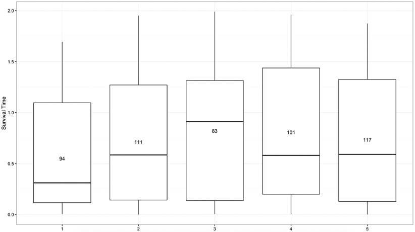
Box plots of survival time by strata index in simulated data generated by the function strata.boosting.
Figure 4:
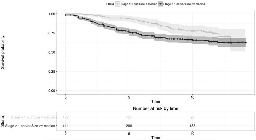
Survival curves for the two strata based on cancer stage and tumor size.
Figure 5:
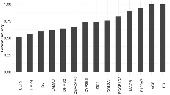
Selection frequencies for genes or phenotype variables that were selected at least 50% of the time with stability selection.
Table 3:
Results from simulation with approximately 1,500 observations and 4,000 possible variables for selection with 100 true signals. The table presents averages with the standard deviation from 50 simulated datasets.
| stopping method |
number selected |
Se | Sp | FDR | MSE | number of iterations |
runtime (seconds) |
|
|---|---|---|---|---|---|---|---|---|
| SurvBoost | fixed | 104 (3) | 0.94 (.02) | 1.00 (.00) | 0.10 (.02) | 381 (.45) | 500 (0) | 138 (11) |
| mboost | 98 (4) | 0.89 (.03) | 1.00 (.00) | 0.10 (.03) | 384 (.36) | 500 (0) | 220 (198) | |
| SurvBoost | cv | 141 (7) | 1.00 (.00) | 0.99 (.00) | 0.29 (.04) | 298 (1) | 5010 (0) | 6531 (18) |
| SurvBoost | # selected | 100 (0) | 0.91 (.02) | 1.00 (.00) | 0.10 (.02) | 382 (2) | 452 (62) | 151 (18) |
| SurvBoost | likelihood | 109 (3) | 0.98 (.01) | 1.00 (.00) | 0.10 (.03) | 382 (.54) | 668 (14) | 216 (18) |
| SurvBoost | EBIC | 112 (4) | 0.99 (.01) | 1.00 (.00) | 0.11 (.03) | 366 (1) | 999 (.25) | 530 (27) |
Table 4:
Stopping criteria options for boosting_core function.
| Call | Method |
|---|---|
| boosting_core(formula, data) | fixed mstop = 500 |
| boosting_core(formula, data, num_iter=1000) | fixed mstop = specified value |
| boosting_core(formula, data, control_method="cv") | 10-fold cross validation |
| boosting_core(formula, data, control_method="num_selected", control_parameter = 5) | number selected, need to specify number of variables |
| boosting_core(formula, data, control_method="likelihood") | change in likelihood |
| boosting_core(formula, data, control_method="BIC") | minimum BIC or EBIC |
| boosting_core(formula, data, control_method="AIC") | minimum AIC |
Table 5:
Functions available in SurvBoost package. Every function accepts a boosting object input to generate the corresponding result.
| Function | Result |
|---|---|
| summary.boosting() | prints summary of variable selection and estimation |
| plot.boosting() | plots variable selection frequency |
| predict.boosting() | generates predicted hazard ratio for each observation or new data |
| post.selection.fitting.boosting() | refits model with only subset of selected covariates |
Acknowledgments
The authors would like to thank the editor and reviewers for suggestions that led to an improved manuscript. This work was partially supported by the NIH grants R01MH105561 (Kang) and R01GM124061 (Kang).
Bibliography
- Al-Haddad S, Zhang Z, Leygue E, Snell L, Huang A, Niu Y, Hiller-Hitchcock T, Hole K, Murphy LC, and Watson PH. Psoriasin (s100a7) expression and invasive breast cancer. The American journal of pathology, 155(6):2057–2066, 1999. [p115] [DOI] [PMC free article] [PubMed] [Google Scholar]
- Allaire J, Francois R, Ushey K, Vandenbrouck G, Geelnard M, and Intel. RcppParallel: Parallel Programming Tools for ‘Rcpp’, 2018. URL https://CRAN.R-project.org/package=RcppParallel. R package version 4.4.0. [p109] [Google Scholar]
- Blumenthal RD, Leon E, Hansen HJ, and Goldenberg DM. Expression patterns of ceacam5 and ceacam6 in primary and metastatic cancers. BMC Cancer, 7(1):2, January 2007. doi: 10.1186/1471-2407-7-2. URL 10.1186/1471-2407-7-2.[p115] [DOI] [PMC free article] [PubMed] [Google Scholar]
- Boersma BJ, Reimers M, Yi M, Ludwig JA, Luke BT, Stephens RM, Yfantis HG, Lee DH, Weinstein JN, and Ambs S. A stromal gene signature associated with inflammatory breast cancer. International Journal of Cancer, 122(6):1324–1332, 2008. doi: 10.1002/ijc.23237. URL 10.1002/ijc.23237. [p115] [DOI] [PubMed] [Google Scholar]
- Bühlmann P and Hothorn T. Boosting algorithms: Regularization, prediction and model fitting (with discussion). Statistical Science, 22(4):477–505, 2007. [p107 ,109] [Google Scholar]
- Bühlmann P and Yu B. Boosting. Wiley Interdisciplinary Reviews: Computational Statistics, 2(1):69–74, 2010. doi: 10.1002/wics.55. URL 10.1002/wics.55. [p105] [DOI] [Google Scholar]
- Chakrabarti R, Hwang J, Blanco MA, Wei Y, Lukacisin M, Romano R-A, Smalley K, Liu S, Yang Q, Ibrahim T, Mercatali L, Amadori D, Haffty BG, Sinha S, and Kang Y. Elf5 inhibits the epithelial-mesenchymal transition in mammary gland development and breast cancer metastasis by transcriptionally repressing snail2. Nature Cell Biology, 14:1212–1222, 2018/February/7/ 2012. [p115] [DOI] [PMC free article] [PubMed] [Google Scholar]
- Chin K, DeVries S, Fridlyand J, Spellman PT, Roydasgupta R, Kuo W-L, Lapuk A, Neve RM, Qian Z, Ryder T, Chen F, Feiler H, Tokuyasu T, Kingsley C, Dairkee S, Meng Z, Chew K, Pinkel D, Jain A, Ljung BM, Esserman L, Albertson DG, Waldman FM, and Gray JW. Genomic and transcriptional aberrations linked to breast cancer pathophysiologies. Cancer Cell, 10(6):529–541, 2017/December/18 2006. doi: 10.1016/j.ccr.2006.10.009. URL 10.1016/j.ccr.2006.10.009. [p114] [DOI] [PubMed] [Google Scholar]
- Eddelbuettel D, Francois R, Allaire J, Ushey K, Kou Q, Russell N, Bates D, and Chambers J. Rcpp: Seamless R and C++ Integration, 2018a. URL https://CRAN.R-project.org/package=Rcpp. R package version 0.12.15. [p109] [Google Scholar]
- Eddelbuettel D, Francois R, Bates D, and Ni B. RcppArmadillo: ‘Rcpp’ Integration for the ‘Armadillo’ Templated Linear Algebra Library, 2018b. URL https://CRAN.R-project.org/package=RcppArmadillo. R package version 0.8.400.0.0. [p109] [Google Scholar]
- Goeman JJ. L1 penalized estimation in the cox proportional hazards model. Biometrical Journal, 52(1): 70–84, 2010. doi: 10.1002/bimj.200900028. [p105] [DOI] [PubMed] [Google Scholar]
- He K, Li Y, Zhu J, Liu H, Lee JE, Amos CI, Hyslop T, Jin J, Lin H, Wei Q, and Li Y. Componentwise gradient boosting and false discovery control in survival analysis with high-dimensional covariates. Bioinformatics, 32(1):50–57, 2016. doi: 10.1093/bioinformatics/btv517. URL 10.1093/bioinformatics/btv517. [p107] [DOI] [PMC free article] [PubMed] [Google Scholar]
- Hofner B, Mayr A, Robinzonov N, and Schmid M. Model-based boosting in R: A hands-on tutorial using the R package mboost. Computational Statistics, 29:3–35, 2014. [p107] [Google Scholar]
- Hothorn T, Buehlmann P, Kneib T, Schmid M, and Hofner B. mboost: Model-Based Boosting, 2017. URL https://CRAN.R-project.org/package=mboost. R package version 2.8-1. [p105] [Google Scholar]
- Jiang W. Process consistency for adaboost. Ann. Statist, 32(1):13–29, February 2004. doi: 10.1214/aos/1079120128. URL 10.1214/aos/1079120128. [p107] [DOI] [Google Scholar]
- Krijgsman O, Roepman P, Zwart W, Carroll JS, Tian S, de Snoo FA, Bender RA, Bernards R, and Glas AM. A diagnostic gene profile for molecular subtyping of breast cancer associated with treatment response. Breast Cancer Research and Treatment, 133(1):37–47, May 2012. doi: 10.1007/s10549-011-1683-z. URL 10.1007/s10549-011-1683-z. [p115] [DOI] [PubMed] [Google Scholar]
- Meinshausen N and Bühlmann P. Stability selection. Journal of the Royal Statistical Society: Series B (Statistical Methodology), 72(4):417–473, 2010. doi: 10.1111/j.1467-9868.2010.00740.x. URL 10.1111/j.1467-9868.2010.00740.x.[p114] [DOI] [Google Scholar]
- Miller LD, Smeds J, George J, Vega VB, Vergara L, Ploner A, Pawitan Y, Hall P, Klaar S, Liu ET, and Bergh J. An expression signature for p53 status in human breast cancer predicts mutation status, transcriptional effects, and patient survival. Proceedings of the National Academy of Sciences of the United States of America, 102(38):13550–13555, 2005. doi: 10.1073/pnas.0506230102. URL 10.1073/pnas.0506230102. [p114] [DOI] [PMC free article] [PubMed] [Google Scholar]
- Naderi A, Teschendorff AE, Barbosa-Morais NL, Pinder SE, Green AR, Powe DG, Robertson JFR, Aparicio S, Ellis IO, Brenton JD, and Caldas C. A gene-expression signature to predict survival in breast cancer across independent data sets. Oncogene, 26:1507–1516, August 2006. [p114] [DOI] [PubMed] [Google Scholar]
- Simon N, Friedman J, Hastie T, and Tibshirani R. Regularization paths for cox’s proportional hazards model via coordinate descent. Journal of Statistical Software, Articles, 39(5):1–13, 2011. doi: 10.18637/jss.v039.i05. URL 10.18637/jss.v039.i05. [p105, 107] [DOI] [PMC free article] [PubMed] [Google Scholar]
- Therneau TM. survival: Survival Analysis, 2017. URL https://CRAN.R-project.org/package=survival. R package version 2.41-3. [p109] [Google Scholar]
- Tibshirani R. The lasso method for variable selection in the cox model. Statistics in medicine, 16(4): 385–395, 1997. [p105] [DOI] [PubMed] [Google Scholar]
- Tozlu S, Girault I, Vacher S, Vendrell J, Andrieu C, Spyratos F, Cohen P, Lidereau R, and Bieche I. Identification of novel genes that co-cluster with estrogen receptor alpha in breast tumor biopsy specimens, using a large-scale real-time reverse transcription-pcr approach. Endocrine-Related Cancer, 13(4):1109–1120, 2006. doi: 10.1677/erc.1.01120. URL 10.1677/erc.1.01120. [p115] [DOI] [PubMed] [Google Scholar]
- Volinsky CT and Raftery AE. Bayesian information criterion for censored survival models. Biometrics, 56(1):256–262, 2000. doi: 10.1111/j.0006-341X.2000.00256.x. URL 10.1111/j.0006-341X.2000.00256.x.[p107] [DOI] [PubMed] [Google Scholar]
- Wang Y, Klijn JG, Zhang Y, Sieuwerts AM, Look MP, Yang F, Talantov D, Timmermans M, Meijer-van Gelder ME, Yu J, et al. Gene-expression profiles to predict distant metastasis of lymph-node-negative primary breast cancer. The Lancet, 365(9460):671–679, 2005. [p115] [DOI] [PubMed] [Google Scholar]
- Yu JX, Sieuwerts AM, Zhang Y, Martens JW, Smid M, Klijn JG, Wang Y, and Foekens JA. Pathway analysis of gene signatures predicting metastasis of node-negative primary breast cancer. BMC Cancer, 7(1):182, 2007. doi: 10.1186/1471-2407-7-182. URL 10.1186/1471-2407-7-182. [p115] [DOI] [PMC free article] [PubMed] [Google Scholar]


