

Abstract
Purpose:
To identify computer-extracted features for central gland and peripheral zone prostate cancer localization on multiparametric magnetic resonance imaging (MRI).
Materials and Methods:
Preoperative T2-weighted (T2w), diffusion-weighted imaging (DWI), and dynamic contrast-enhanced (DCE) MRI were acquired from 23 men with confirmed prostate cancer. Following radical prostatectomy, the cancer extent was delineated by a pathologist on ex vivo histology and mapped to MRI by nonlinear registration of histology and corresponding MRI slices. In all, 244 computer-extracted features were extracted from MRI, and principal component analysis (PCA) was employed to reduce the data dimensionality so that a generalizable classifier could be constructed. A novel variable importance on projection (VIP) measure for PCA (PCA-VIP) was leveraged to identify computer-extracted MRI features that discriminate between cancer and normal prostate, and these features were used to construct classifiers for cancer localization.
Results:
Classifiers using features selected by PCA-VIP yielded an area under the curve (AUC) of 0.79 and 0.85 for peripheral zone and central gland tumors, respectively. For tumor localization in the central gland, T2w, DCE, and DWI MRI features contributed 71.6%, 18.1%, and 10.2%, respectively; for peripheral zone tumors T2w, DCE, and DWI MRI contributed 29.6%, 21.7%, and 48.7%, respectively.
Conclusion:
PCA-VIP identified relatively stable subsets of MRI features that performed well in localizing prostate cancer on MRI.
Keywords: prostate cancer, computer-extracted features, principal component analysis, model interpretation, feature selection
DURING THE PAST DECADE multiparametric (MP) magnetic resonance imaging (MRI) has emerged as the imaging modality of choice for disease staging in patients with biopsy-confirmed prostate cancer (1). Additionally, MRI is becoming more popular for prostate cancer detection and localization in patients with repeated negative biopsies but elevated prostate-specific antigen (PSA) and to facilitate targeted biopsies. Prostate MRI exams typically involve a combination of T2-weighted (T2w) MRI, which provides excellent contrast of anatomic structures due to its sensitivity to fluid content; diffusion-weighted imaging (DWI), which shows tissue microstructure by probing molecular water diffusion; DCE MRI, which is used to evaluate tumor microvasculature and angiogenesis; and MR spectroscopy (MRS), which assesses the presence of various metabolites in the tissue. Prostate cancer manifests on T2w MRI as areas with low signal intensity relative to normal peripheral tissue (2); on DWI as areas with low apparent diffusion coefficient (ADC) values (3); and on DCE MRI as regions with increased contrast enhancement (4). MRS is not routinely acquired at many sites because MRS imaging quality varies greatly between institutions and is associated with high interobserver variability (5).
The prostate gland can be divided into two primary anatomical regions: the peripheral zone (PZ) and the central gland (CG), comprised of the central and transitional zones. Several studies have found that clinical features of prostate cancer vary based on the spatial location of the tumor in the prostate (6). For example, PZ tumors tend to be more aggressive than CG tumors (7). Seventy percent of prostate tumors occur in the PZ, where they appear on T2w MRI as regions of low signal intensity surrounded by brighter normal PZ tissue (8,9). The remaining prostate tumors are found in the CG, where they manifest as homogeneous, lenticular-shaped lesions with low signal intensity (8,9). Moreover, it was recently shown that CG and PZ cancer possess distinct quantitative imaging signatures on MRI (10).
A number of recent studies have shown that computer-extracted MRI features are useful for detecting prostate cancer (10–16). It is thought that computer-extracted features are capable of quantitatively describing tissue microarchitecture and morphology, which provide clues about cancer presence. Most of these efforts have been directed towards training classifiers with computer-extracted features to accurately discriminate between cancer regions and normal prostate tissue. These studies, which use a combination of first-order statistical features, co-occurrence features, and wavelet features, report improved cancer detection accuracy compared to MP MRI signal intensities (10–12).
Some of these studies use 50–300 computer-extracted MRI features for prostate cancer detection (10–13). While it is important to extract a large pool of features that fully describe tissue morphology and microarchitecture on MRI, many of these features may be redundant. Moreover, while some computer-extracted features may be useful for cancer detection in the PZ, others may be better suited for cancer detection in the CG. According to the Hughes effect (17), predictive power reduces as dimensionality increases; this effect, termed the “curse of dimensionality,” is accentuated when the sample size is small. Consequently, when only a limited number of training samples are available, a generalizable classifier cannot be constructed with more than a handful of features (18). In order to construct a generalizable classifier, a small subset of computer-extracted features that best characterize prostate cancer must be identified.
There are two overarching methods for overcoming this “curse of dimensionality”: feature selection (FS) and dimensionality reduction (DR). Although FS is useful for reducing the number of features, both feature ranking processes and greedy FS algorithms tend to be unstable, ie, slight perturbations in data may lead to different sets of selected features (19). Alternatively, DR transforms high-dimensional features into a series of eigenvectors, which are used for classification. However, because eigenvectors are used for classification instead of the original features, it is challenging to understand the role that each feature—and MRI protocol—plays in cancer detection. This lack of interpretability is a serious drawback of DR.
The primary goal of this work is to combine the advantages of both DR and FS to identify a small subset of computer-extracted features that collectively characterize prostate cancer appearance on MP MRI and to evaluate the performance of these features within a decision support classifier for cancer detection and localization. Prostate cancer localization accuracy is assessed by comparing voxel-wise classification results with “ground truth” cancer extent, delineated by a pathologist on ex vivo histology and mapped to in vivo MRI via nonlinear registration (20,21). Toward this end, we present a method for quantifying the extent that a particular feature or set of features contributes to classification on a lowdimensional embedding obtained by principal component analysis (PCA), a popular linear DR algorithm. A secondary goal of this work is to investigate zonal differences in prostate cancer characteristics.
MATERIALS AND METHODS
Data Acquisition
This retrospective study was approved by the Institutional Review Board at Beth Israel Deaconess Medical Center. This study was an arm of a prospective study that included 108 subjects (mean age, 58.5 years; age range, 47–72 years) with biopsy-confirmed prostate cancer (median Gleason score, 7; range, 6–9) who were scheduled for radical prostatectomies. Forty-five subjects were excluded for lack of DCE MRI or corresponding digitized whole mount histological sections (WMHS), and another 40 were excluded because the pathologist did not annotate cancer on the WMHS. A total of 23 cases were included in the current study, of which 15 cases included T2w, DWI, and DCE MRI, while the remaining eight cases included only T2w and DCE MRI.
Before surgery, the patients were imaged using a combined torso-phased array and endorectal coil (MedRad, Pittsburgh, PA) using a 3T whole-body MRI scanner (Genesis Signa LX Excite; GE Medical Systems, Milwaukee, WI). The parameters for axial T2w MRI were repetition time / echo time (TR/TE) = 6375/165 msec, slice thickness of 1.5–2 mm (no gap between slices), and matrix size of 320 × 224–192 voxels with a field of view (FOV) of 12 × 12 cm. The DCE MRI protocol included two precontrast T1-weighted gradient echo images, acquired at 95-second intervals before a bolus injection of 0.1 mmol/kg of gadolinium-DTPA, and five postcontrast images acquired at the same temporal resolution. The DCE MRI parameters were TR/TE = 9.3/4.2 msec, flip angle = 18°, FOV = 14 × 14 cm and matrix size 256 × 224 (interpolated to 256 × 256 matrix), with no phase wrap. Transverse DWI parameters were TR/TE = 6500/80.6 msec, FOV = 24 × 24 cm, matrix size 256 × 192, B-value = 0,1000 s/mm2, two averages and 25 directions. Instead of using more averages, we used 25 directions to improve results in diffusion tensor imaging and anisotropic maps and enhance contrast in ADC maps.
A pathologist (E.M.G., 16 years of experience) and radiologist (B.N.B., 14 years of experience) working in unison visually identified 96 corresponding 2D WMHS and axial MRI slices from these 23 studies. These correspondences were established by means of anatomical fiducials such as the urethra, veromontanum, and prominent nodules of benign prostatic hyperplasia that were visually discernible on both histology and MRI. Based on the recommendations of McNeal (22), each patient was classified as having CG or PZ cancer if more than 70% of the cancer volume was present in a particular zone. To ensure that the sets of CG and PZ cancer were distinct from each other, only sections displaying an explicit tumor focus in either the CG or the PZ were included in this analysis. Based on the zonal locations of the prostate tumors and the MRI protocols available for each patient, four sets of patient studies were composed and analyzed separately in this study (see Table 1).
Table 1.
Description of Four Sets of Patient Studies That Were Analyzed Separately in This Study
| Dataset | Tumor Location | Number of Patients | MRI Protocols |
|---|---|---|---|
| S1 | PZ | 18 | T2w, DCE MRI |
| S2 | PZ | 10 | T2w, DWI, DCE MRI |
| S3 | CG | 5 | T2w, DWI, DCE MRI |
| S4 | PZ + CG | 15 | T2w, DWI, DCE MRI |
Preprocessing of MRI
T2w and DCE MRI were corrected for acquisition-based MRI intensity artifacts that affect image analysis algorithms (16). The most significant artifact is the bias field on T2w and DCE MRI, which occurs due to usage of an endorectal probe (23). Bias field artifacts were corrected by the N3 algorithm (24), which incrementally deconvolves smooth bias field estimates from acquired image data (see Fig. 1). A second artifact, intensity non-standardness (25), refers to the issue of inter- and intrapatient MRI “intensity drift,” which causes MRI intensities to lack tissue-specific numeric meaning (25). This artifact was corrected by interactive implementation of the generalized scale algorithm (25), which aligns image intensity histograms across different MRI studies, thereby enabling MRI intensities to have a consistent tissue-specific numeric meaning (see Fig. 1).
Figure 1.
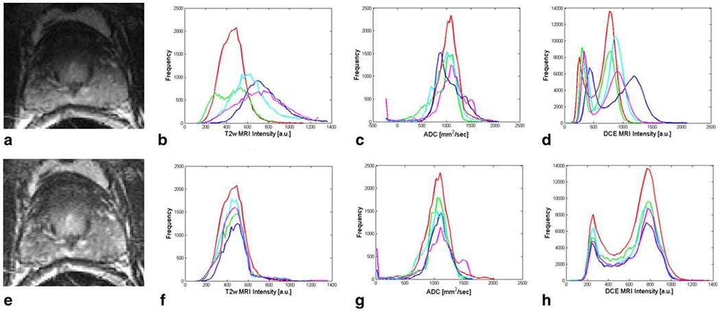
A T2w MR image is shown (a) before and (e) after correction of bias field inhomogeneities. Signal intensity histograms associated with several patients are shown before and after intensity standardization for T2w MRI in (b) and (f), ADC maps in (c) and (g), and DCE MRI in (d) and (h), respectively. [Color figure can be viewed in the online issue, which is available at wileyonlinelibrary.com.]
Registration of MRI and WMHS Slices
In order to obtain “ground truth” annotation of prostate cancer extent on in vivo MRI, nonlinear registration of MP MRI and WMHS was performed (20,21). First, T2w MRI and ADC maps obtained from DWI were spatially aligned with DCE MRI via volumetric affine registration, which corrected interacquisition movement and interprotocol resolution differences. Slice correspondences between T2w, DCE, and ADC images, as well as relative voxel locations and sizes, were determined using DICOM image header information. After interprotocol alignment, all MRI data were analyzed at the DCE MRI resolution.
Once T2w, DCE, and ADC images were spatially aligned, in vivo MRI was registered with ex vivo WMHS. Registration of WMHS and MRI is complicated by differences in image intensities and nonlinear changes in the shape of the prostate due to both the endorectal coil and deformations to the histological sections upon fixation and sectioning. We therefore used a nonrigid registration scheme (20) driven by a higher-order variant of mutual information that handles images with very different intensities (eg, MRI and WMHS data) and deformation characteristics (eg, in vivo to ex vivo). First, affine alignment of WMHS to the corresponding T2w MRI slice was performed to correct large translation, rotation, and scale differences. Then the rigid alignment of WMHS and T2w MRI was improved by means of a fully automated nonlinear hierarchical B-spline mesh grid image warping scheme (20).
After corresponding 2D WMHS slices were aligned with MRI, the spatial extent of the cancer was mapped from WMHS slices onto corresponding MRI slices. The spatial extent of the cancer mapped onto MRI was examined and manually corrected (as required) by a radiologist (N.B.B., 14 years of experience) using Photoshop (Adobe Systems, San Jose, CA). The final result was a labeling of each MRI voxel within the prostate as corresponding to cancer or benign prostate tissue (see Fig. 2).
Figure 2.
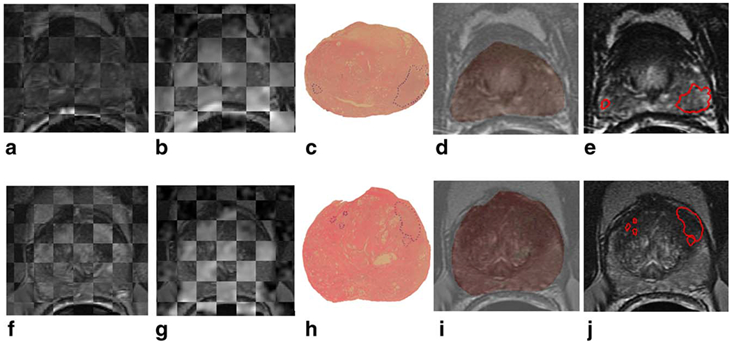
Checkerboard images illustrating registration of T2w MRI and DCE MRI images are shown in (a) and (f) for patients with PZ cancer and CG cancer, respectively; registration of T2w MRI and ADC maps is shown in (b) and (g). The original 2D whole-mount histological sections, with prostate cancer extent outlined in blue by a pathologist, are shown in (c) and (h), and overlays of WMHS and T2w MRI after nonlinear multimodal registration are shown in (d) and (i). Mapped cancer extent on T2w MRI, outlined in red, is shown in (e) and (j). [Color figure can be viewed in the online issue, which is available at wileyonlinelibrary.com.]
MP MRI Feature Extraction
Signal intensity (SI) features considered in this study included T2w MRI intensities, time-resolved DCE MRI signal intensities and tissue concentration curves, estimated using the method of Medved et al (26), and ADC values for the studies with available ADC maps (see Table 2). Additionally, we computed a large number of computer-extracted features that have previously been used for prostate cancer detection on T2w MRI (10). These 112 features, which we extracted on a per-voxel basis from both T2w MRI and ADC maps, are described briefly in Table 3. Additionally, six kinetic features (27) were obtained for each DCE MRI voxel (Table 3). All feature extraction was implemented using MatLab (MathWorks, Natick, MA).
Table 2.
Description of MP MRI Signal Intensity Features Used for CG and PZ Prostate Cancer Localization and Their Associated PCA-VIP Scores
| Feature | Amount | Significance for Prostate Cancer Localization | PCA-VIP (PZ) | PCA-VIP (CG) |
|---|---|---|---|---|
| T2w MRI SI | 1 | T2w MRI SI is low in tumors relative to surrounding normal tissue. | 0.68 | 0.60 |
| ADC | 1 | ADC values are low in tumors due to increased cell density and tissue disorganization in tumors. | 0.91 | 0.81 |
| DCE MRI SI | 6 | High microvessel density in tumor regions leads to increased contrast enhancement compared to normal peripheral tissue. | Total: 2.39 | Total: 2.28 |
| Contrast agent concentration | 6 | Due to increased angiogenesis, contrast agent uptake is faster in tumors than surrounding normal tissue. | Total: 0.82 | Total: 0.76 |
SI, signal intensity.
Table 3.
Description of Features Computed on a Per-Pixel Basis From MP MRI and the Motivation for Using Them for Prostate Cancer Localization
| Feature | Amount | Description | Significance for Prostate Cancer Localization |
|---|---|---|---|
| First-order statistics | 14 T2w + 14 ADC | Mean, standard deviation, and range of intensities, as well as non-steerable gradient features obtained by convolution with Sobel and Kirsch operators | Localize image regions with significant SI changes and accurately detect region boundaries |
| Co-occurrence features | 36 T2w + 36 ADC | Statistical features computed from the joint probability distribution of intensity value co-occurrences | Differentiate between homogeneous regions of low SI of prostate cancer and hyper-intense normal prostate |
| Gabor wavelet coefficients | 48 T2w + 48 ADC | Multi-orientation features computed from a Gaussian function convolved with a sinusoid | Quantify features qualitatively assessed by radiologists when examining appearance of the carcinoma |
| Haar wavelet coefficients | 12 T2w + 12 ADC | Multi-level coefficients from Haar wavelet decomposition | Accentuate amorphous nature of non-cancer regions within foci of low SI |
| Kineticfeatures | 6 DCE | Kinetic characteristics computed from DCE MRI SI curves | Discriminate between perfusion characteristics of angiogenic and non-angiogenic regions |
SI, signal intensity.
Notation
We define a voxel in the MR image as c ∈ C. Each c ∈ C is associated with a label y(c) ∈ {0,1}, where y(c) = 0 if voxel c is benign and y(c)=1 otherwise. For prostate studies in dataset S1 each c ∈ C is also associated with the feature vector F(c) = [FT2w(c), FDCE(c)], where FT2w(c) and FDCE(c) are comprised of features extracted from T2w MRI and DCE MRI, respectively. For datasets S2, S3, and S4 the feature vector associated with each c ∈ C is F(c) = [FT2w(c), FADC(c),FDCE(c)], where FADC(c) contains features extracted from ADC maps. A subset of features in F(c) is denoted as , where and M is the cardinality of F(c).
Principal Component Analysis
PCA (28) involves finding a linear transformation that maximizes the variance in data and applying this transformation to obtain uncorrelated features. The data matrix X is constructed with the N M-dimensional feature vectors F(c), normalized to the interval [0,1], as rows. The orthogonal eigenvectors of X, which express the variance in the data, become the principal components. Thus, PCA forms the following model:
| [1] |
where T contains the M principal component vectors ti as columns and P⊺ is comprised of the M loading vectors pi as rows. DR is accomplished by retaining only the first m principal components and loading vectors, which comprise most of the variance in the data.
Variable Importance in PCA Projections
The importance of a feature to classification on a PCA embedding is a function of its impact on the shape of the PCA embedding and its value in predicting class labels. Consequently, we propose the following expression to quantify the importance of features to classification on the embedding:
| [2] |
where bi are coefficients that solve the regression equation
| [3] |
which relates the principal component scores to the outcome vector y. This expression is derived from a similar expression that was introduced to quantify the contributions of features to a partial least squares embedding (29). In Eq. [2] the fraction reveals how much the ith principal component depends on the jth feature. The overall importance of the ith feature can be calculated by summing its contributions to each dimension of the PCA embedding and weighting these values by 1) the regression coefficients bi, which relate the data back to the class labels, and 2) the transformed data ti. Thus, although PCA is itself an unsupervised method, the exploitation of class labels in computing the PCA-VIP scores leads to the identification of features that provide good class discrimination. The degree to which a feature contributes to classification in the PCA embedding space is directly proportional to the square of its PCA-VIP score. Thus, features with the highest PCA-VIP scores contribute most to class discrimination on the PCA embedding.
Determination of Intrinsic Dimensionality
The intrinsic dimensionality of the data, m, (ie, the number of principal components retained during dimensionality reduction) was determined based on the effect of the value of m on the resulting PCA-VIP scores, as follows. Beginning with m = 1, m was gradually increased; as a result, the PCA-VIP scores fluctuated due to the consideration of features’ effects on more principal components. Once varying m no longer significantly impacted the PCA-VIP scores (p > 0.05), m was determined to be sufficiently high. This value of m, typically m < 10, determined how many principal components were retained.
Relative Importance of Feature Subsets
The importance of a feature subset is quantified as:
| [4] |
It follows that the relative importance of subset compared to subset can be expressed as:
| [5] |
Because , the relative importance of subset compared to the entire feature set can be expressed simply as .
Evaluation
PCA-VIP was evaluated in terms of its ability to find a subset of features that 1) remains stable (ie, robust to perturbations in the data) and 2) provides high accuracy in cancer localization. The stability of PCA-VIP was evaluated by the Jaccard index (30):
| [6] |
If an FS algorithm is stable, repeated implementations will lead to similar feature subsets and a Jaccard index close to 1. In this study we compared the stability of PCA-VIP with minimum-redundancy-maximum-relevance (mRMR) (31), a popular FS scheme.
Classification accuracy was evaluated by using two Bayesian classifiers (28): the parametric logistic regression classifier and the nonparametric naïve Bayes classifier. Based on the voxel-wise prediction results obtained from these classifiers, receiver operating characteristic (ROC) curves representing the tradeoff between cancer detection sensitivity and specificity were generated. The area under the ROC curve (AUC) was used to evaluate classifier accuracy in conjunction with different feature subsets. In order to ensure robustness of AUC estimates, a 3-fold randomized cross-validation procedure, using approximately 2/3 of the patient studies for training and the remaining 1/3 for testing, was repeated 30 times, and the average AUC and J values were obtained.
RESULTS
Features Selected by PCA-VIP
Table 4 lists the 10 features with the highest PCA-VIP scores for PZ and CG cancer localization; these features constituted and , respectively. Note that two features are shared by and : the enhancement ratio from DCE MRI and a Haar wavelet coefficient derived from DWI. Whereas included eight co-occurrence features extracted from T2w MRI, contained mainly Gabor and Haar wavelet features and no co-occurrence features. Half of the features in were derived from DWI, three from T2w MRI and two from DCE MRI: enhancement ratio and time-to-peak.
Table 4.
The Top 10 Computer-Extracted Features
| Dataset | MRI Protocol | Feature | PCA-VIP score |
|---|---|---|---|
| PZ tumors | T2w MRI | Haar: Horizontal coefficient (level 4) | 2.25 |
| Gabor (orient = 90°, wavelength=45.2548) | 1.59 | ||
| Haar: Horizontal coefficient (level 3) | 1.53 | ||
| DWI MRI | Haar: Horizontal coefficient (level 4) | 2.34 | |
| Haar: Horizontal coefficient (level 3) | 1.83 | ||
| Gabor (orient=22.5°, wavelength=45.2548) | 1.64 | ||
| Gabor (orient=90°, wavelength=22.6274) | 1.53 | ||
| Gabor (orient=90°, wavelength=45.2548) | 1.50 | ||
| DCE MRI | Enhancement ratio | 1.89 | |
| Time to peak | 1.67 | ||
| CG tumors | T2w MRI | Co-occurrence: Inertia (w=7) | 2.38 |
| Co-occurrence: Difference average (w=7) | 2.32 | ||
| Co-occurrence: Difference variance (w=7) | 2.26 | ||
| Co-occurrence: Difference average (w=5) | 2.15 | ||
| Co-occurrence: Difference variance (w=5) | 1.96 | ||
| Co-occurrence: Inverse difference moment (w=5) | 1.94 | ||
| Co-occurrence: Inverse difference moment (w=7) | 1.93 | ||
| Co-occurrence: Inertia (w=5) | 1.89 | ||
| DWI MRI | Haar: Horizontal coefficient (level 4) | 2.27 | |
| DCE MRI | Enhancement ratio | 2.83 |
Features that contribute the most to prostate cancer localization on a PCA embedding, obtained by voting among the top 10 selected features in 30 runs of cross-validation, are listed for PZ and CG tumors. Their associated PCA-VIP scores are obtained by averaging across the 30 cross-validation runs (w stands for window size, an associated parameter setting for the feature).
Stability of PCA-VIP Feature Subsets
Figure 3 displays the Jaccard index for feature subsets selected by PCA-VIP and mRMR. For all four datasets, the Jaccard index was higher for PCA-VIP than mRMR. For datasets S2, S3, and S4, this difference was statistically significant. In particular, the Jaccard index associated with PCA-VIP for CG cancer localization (dataset S3) was as high as 0.68, signifying that the feature subset selected by PCA-VIP for CG cancer localization was highly stable and relatively unaffected by perturbations in the data.
Figure 3.
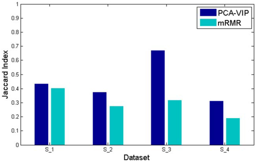
The Jaccard index, used to assess the stability of selected feature subsets, is compared when PCA-VIP and mRMR are employed to select the top 10 features. [Color figure can be viewed in the online issue, which is available at wileyonlinelibrary.com.]
Classification Accuracy Provided by Selected Features
AUC values obtained by using and in conjunction with logistic regression and naïve Bayes classifiers followed similar trends (see Fig. 4c,d), although the logistic regression classifiers generally provided higher AUC values than the naïve Bayes classifier. Figure 5f,l, respectively, illustrate the accuracy with which logistic regression classifiers constructed in conjunction with and localize cancer on MRI. In contrast to classifiers using all of the computer-extracted features (see Fig. 5d,j), the classifiers that used only the features selected by PCA-VIP accurately identified both the tumor location and the approximate size and shape of the lesion. When was used in conjunction with logistic regression to classify voxels as cancer or benign, an AUC value of 0.85 was achieved (Fig. 4d); when a logistic regression classifier was used in conjunction with , an AUC of 0.79 was obtained (Fig. 4d). In contrast, when features extracted from DWI were not available (dataset S1), the average AUC using the entire dropped to 0.75. When PCA-VIP was used to select features for cancer detection independent of zonal prostate location, AUC values were substantially reduced (Fig. 4c,d).
Figure 4.
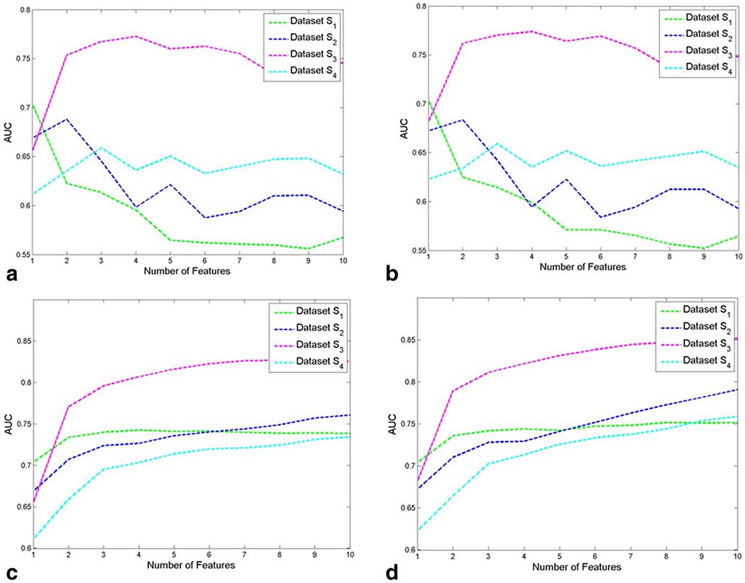
AUC values, averaged across 30 cross-validation runs, are plotted for each of the top 10 computer-extracted features for (a) a naïve Bayes classifier and (b) a logistic regression classifier. The AUCs that arise when aggregating the top 1–10 computer-extracted features for classification are shown in (c) for a naïve Bayes classifier and in (d) for a logistic regression classifier.
Figure 5.
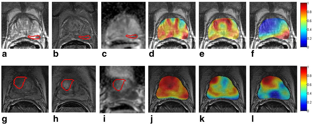
Ground truth extent of prostate cancer is delineated on T2w MRI in red for a representative slice of (a) a PZ tumor and (g) a CG tumor. Corresponding DCE MR images at peak contrast enhancement and ADC maps are shown in (b) and (h) and in (c) and (i), respectively. Heatmaps representing the pixel-wise probability of cancer presence, obtained via logistic regression classification, are shown in (d) and (j) using all of the computer-extracted features, (e) and (k) using signal intensity features, and (f) and (l) using and , respectively. Red indicates a high probability of cancer presence, yellow indicates a low probability of cancer presence, and blue indicates no cancer presence.
Comparison of Signal Intensity and Computer-Extracted Features
The PCA-VIP scores associated with each of the SI features are listed in Table 2; none of the SI features was associated with PCA-VIP scores greater than 1, indicating that they contributed less to prostate cancer localization than the feature with the mean PCA-VIP score. In contrast, PCA-VIP scores associated with the top-performing computer-extracted features, listed in Table 4, ranged from 1.5 to 2.83. Figures 5b and 3f illustrate that logistic regression classifiers constructed in conjunction with SI features allowed for localization of PZ and CG cancer, respectively, with high sensitivity but poor specificity. In contrast, logistic regression classifiers constructed in conjunction with and localized cancer with high sensitivity and specificity (Fig. 5f,l).
Ranking MRI Protocols for Prostate Cancer Localization
The relative contributions of T2w, DWI, and DCE MRI features to cancer localization were assessed using Eq. [5]. For CG cancer localization T2w MRI features contributed nearly twice as much to classification accuracy in the PCA embedding space as DWI features (Fig. 6a). When only features comprising were considered (Fig. 6b), T2w MRI features contributed almost 70% of the classification performance, with DCE MRI features contributing ~20% and DWI features contributing ~10% (ie, each of the 10 features contributes ~10%). For PZ cancer localization, however, features extracted from both T2w MRI and ADC maps had nearly identical contributions to classification accuracy in the PCA embedding space (dataset S2, Fig. 6a). When only features comprising were considered (Fig. 6b), DWI MRI features contributed almost 50% of the classification performance, with DCE MRI features contributing ~20% and T2w features contributing nearly 30%.
Figure 6.
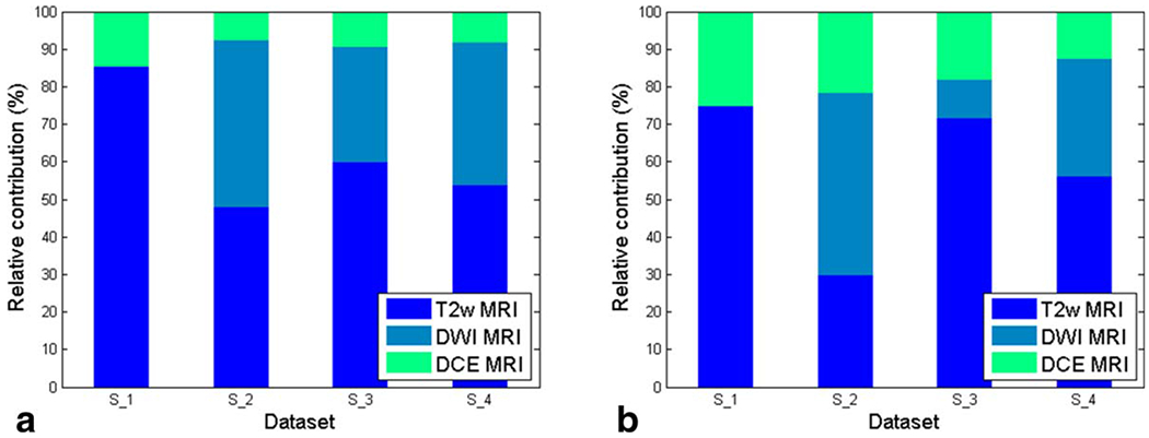
Relative importance of (a) all features and (b) features in and extracted from T2w, DWI, and DCE MRI for each dataset. [Color figure can be viewed in the online issue, which is available at wileyonlinelibrary.com.]
DISCUSSION
The primary contribution of this work is a means of identifying computer-extracted MRI features for prostate cancer localization while circumventing the “curse of dimensionality.” This was made possible via a new PCA-VIP scheme, which involves mapping the high-dimensional data via PCA and subsequently ranking features based on their contributions to both the structure of the PCA embedding and class labels. PCA-VIP was implemented to identify computer-extracted MRI features and MRI protocols that are most useful for prostate cancer detection and localization depending on zonal tumor location.
It is important to note that PCA-VIP differs from other FS methods, such as stepwise and greedy FS algorithms, in two key ways. First, whereas FS algorithms are typically used to identify a feature subset that will, in turn, drive a classification task, PCA-VIP is designed for interpreting a classifier that was already constructed in a reduced-dimensional setting. Second, whereas other FS algorithms select features based on maximizing a criterion like mutual information or classification accuracy, PCA-VIP is currently the only FS scheme that selects features based on their roles in 1) defining the geometry of an unsupervised low-dimensional embedding and 2) driving accurate classification.
In order to ensure that features identified by PCA-VIP are truly predictive of cancer presence, PCA-VIP was evaluated in terms of its ability to identify a stable set of features that provides high accuracy in localizing prostate cancer on MRI. The stability of the feature subsets selected by PCA-VIP was assessed using the Jaccard index and compared with mRMR, a popular FS method. The Jaccard index was higher for PCA-VIP than mRMR for all four datasets considered in this work, and this difference was statistically significant for datasets S2, S3, and S4. Nevertheless, while the Jaccard index associated with (dataset S3) was especially high (0.68), the Jaccard index associated with (datasets S1 and S2) was only mediocre (0.38–0.43). This may be attributed to the fact that the CG tumors considered in this study shared similar characteristics, while the PZ tumors considered in our study were more diverse in terms of shape, size, location, and tumor microarchitecture and morphology.
The predictive power of the features selected by PCA-VIP was evaluated by AUC values associated with naïve Bayes and logistic regression classifiers that were constructed in conjunction with and for voxel-wise cancer localization. Regardless whether a naïve Bayes or a logistic regression classifier was used, AUC values obtained using and were high (0.73–0.85) and comparable with other studies, which reported AUC values ranging from 0.73 to 0.86 (10,11). In comparison, studies that used MRI features to discriminate between cancerous lesions and normal regions-of-interest reported AUC values ranging from 0.71 to 0.94 (13,32,33). Nevertheless, we found that AUC values were higher for CG cancer localization than for PZ cancer localization. This trend, which was previously reported by Viswanath et al (10), may be attributed to the fact that the CG tumors analyzed in our study were similar in size and located in the same region of the CG, whereas the PZ tumors varied considerably.
The types of features identified by PCA-VIP as useful for cancer localization were found to depend on the spatial location of the tumor in the prostate. For example, while was comprised primarily of co-occurrence texture features and included only one wavelet feature, contained many Gabor and Haar wavelet features but no co-occurrence features. The importance of these steerable filters suggests that perhaps PZ tumors manifest a textural orientedness that is not manifested by CG tumors. Among the features extracted from DCE MRI, time-to-peak was found to be useful for cancer localization in the PZ but not in the CG. In contrast, the signal enhancement ratio, which was previously shown to be informative for breast cancer localization (34), was one of only two features identified by PCA-VIP as useful for tumor localization in both the CG and the PZ. It is important to note that although time-to-peak was not included in (because co-occurrence features extracted from T2w MRI had higher PCA-VIP scores), the PCA-VIP score associated with time-to-peak for CG tumor localization (1.86) is higher than the PCA-VIP score associated with time-to-peak for PZ tumor localization (1.67). This finding is supported by Sung et al (36), who found that time-to-peak was a better independent predictor of cancer presence in the CG than in the PZ. Our finding that nearly distinct subsets of computer-extracted features are useful for prostate cancer localization in the CG and PZ, respectively, appears to corroborate previous studies that have suggested that PZ and CG tumors have distinct appearances on MRI (2,8–10).
Previous studies have reported improved prostate cancer detection and localization accuracy when computer-extracted MRI features are used in addition to MRI signal intensities (11,13). Using the PCA-VIP scheme we quantitatively compared the relative contributions of MRI signal intensities and computer-extracted features. Computer-extracted features from T2w MRI and ADC maps were found to be more predictive of cancer localization than T2w MRI signal intensities and ADC values, which were associated with low PCA-VIP scores for both CG and PZ cancer localization. Among DCE MRI features, several computer-extracted kinetic features were associated with high PCA-VIP scores, while the original time-resolved intensity values and tissue concentration curves were not. The relatively low importance of many of the DCE MRI features may be attributed to the fact that our DCE MRI data were of very low temporal resolution (95 sec).
A number of studies (35–39) have explored the added benefit of MP MRI, in comparison to T2w MRI alone for prostate cancer detection but have reported contradictory results. For example, while some have reported that combining ADC maps and T2w MRI improves cancer detection when compared to T2w MRI alone (36–39), others found that the addition of ADC maps does not significantly improve cancer detection (38). In our study the PCA-VIP scheme was employed to quantify how much each MRI protocol contributed to accurate cancer localization in both the CG and the PZ. For CG cancer localization, T2w MRI features contributed almost twice as much as DWI features; when only the features in are considered, features extracted from T2w MRI contributed more than five times as much as DWI features. Thus, although it is well established that ADC values are more predictive of cancer presence than T2w signal intensities (32,33), texture features extracted from T2w MRI appear to be more predictive of CG cancer presence than both ADC values and ADC texture features. In contrast, for PZ tumor localization computer-extracted features from both T2w MRI and ADC maps contributed substantially to classification performance. Our finding that ADC maps are more beneficial for localizing PZ tumors than CG tumors may be attributed to a higher DWI signal-to-noise ratio near the endorectal coil. We note that although DCE MRI features comprised only 3% of the features explored in this study, they played a large role in localization of both CG and PZ cancer.
There were a few limitations to our study. First, our patient cohort was small, consisting of only 10 PZ tumors and 5 CG tumors with T2w, DWI, and DCE MRI and an additional 8 PZ tumors with only T2w and DCE MRI. Although this small cohort size is similar to other studies (11,13,33), the small sample size does have ramifications with regard to classifier generalizability. Applying PCA is helpful for building a classifier when the sample size is small and the data dimensionality is high; however, even PCA can be subject to the Hughes effect, causing instability of the PCA embedding when the sample size is too small (40). In our study, the PCA embedding was somewhat unstable because of the small cohort size; this led to some instability in PCA-VIP scores and hence feature sets selected based on PCA-VIP scores. A second limitation was the fact that we did not quantitatively evaluate the coregistration of MRI and histology. Some error may have been introduced in the determination of the slice correspondences between histology sections and MRI slices and may have affected the determination of “ground truth” cancer extent. Nevertheless, we believe that our coregistration was more rigorous than previous studies that manually delineated cancer regions on MRI by visual registration with pathology information (11,13,33). Third, PCA-VIP is limited by the fact that it is an unsupervised, linear DR method. Because PCA is unsupervised, the PCA embedding may be driven by differences between normal CG and PZ, as well as differences between cancer and normal prostate regions. Consequently, it is possible that some features that are highly predictive of cancer presence may not be identified by PCA-VIP. Additionally, because PCA considers only linear correlations between features, it is possible that a different set of features may be selected if the VIP scheme were applied to an embedding obtained from a nonlinear DR scheme. However, currently VIP is only mathematically valid in conjunction with PCA and PLS. A final limitation is our choice of computer-extracted features. Although we endeavored to extract a comprehensive collection of computer-extracted features, we could not include all possible image features, such as local binary pattern and histogram of gradient features. Nevertheless, the PCA-VIP scheme is a general framework to identify the relative contributions of any available MRI protocols and MRI features to accurate cancer localization.
In conclusion, we presented PCA-VIP for assessing the contributions of individual features to classification on a PCA embedding and demonstrated that PCA-VIP enables the identification of computer-extracted MRI features that are useful for prostate cancer localization. This work is the first attempt to quantify the contributions of individual features and MRI protocols to cancer localization when DR is implemented to circumvent the “curse of dimensionality.” In addition to identifying computer-extracted features that are predictive of cancer presence on MRI, we found that CG and PZ cancer have distinct attributes that do not necessarily manifest via the same MRI protocols. Future work will involve the collection of data from a larger cohort of patients; this should provide a more generalizable PCA embedding and hence a more stable set of selected features. Additionally, future studies will assess the benefit of placing maps of the computer-extracted features identified by PCA-VIP alongside MP MR images in decision support systems to aid radiologists in prostate cancer detection.
Acknowledgments
Supported by the National Cancer Institute of the National Institutes of Health under award numbers R01CA136535-01, R01CA140772-01, and R21CA167811-01; the National Institute of Biomedical Imaging and Bioengineering of the National Institutes of Health under award number R43EB015199-01; the National Science Foundation under award number IIP-1248316; the QED award from the University City Science Center and Rutgers University; and the National Science Foundation Graduate Research Fellowship.
Footnotes
View this article online at wileyonlinelibrary.com.
REFERENCES
- 1.Schiebler ML, Schnall MD, Pollack HM, et al. Current role of MR imaging in the staging of adenocarcinoma of the prostate. Radiology 1993;189:339–352. [DOI] [PubMed] [Google Scholar]
- 2.Akin O, Sala E, Moskowitz CS, et al. Transition zone prostate cancers: features, detection, localization, and staging at endorectal MR imaging. Radiology 2006;239:784–792. [DOI] [PubMed] [Google Scholar]
- 3.Padhani AR, Liu G, Mu-Koh D, et al. Diffusion-weighted magnetic resonance imaging as a cancer biomarker: consensus and recommendations. Neoplasia 2009;11:102–125. [DOI] [PMC free article] [PubMed] [Google Scholar]
- 4.Cornud F, Delongchamps NB, Mozer P, et al. Value of multiparametric MRI in the work-up of prostate cancer. Curr Urol Rep 2012;13:89–92. [DOI] [PubMed] [Google Scholar]
- 5.Weinreb JC, Blume JD, Coakley FV, et al. Prostate cancer: sextant localization at MR imaging and MR spectroscopic imaging before prostatectomy—results of ACRIN prospective multi-institutional clinicopathologic study. Radiology 2009;251:122–133. [DOI] [PMC free article] [PubMed] [Google Scholar]
- 6.Stamey TA, Yemoto CM, McNeal JE, Sigal BM, Johnstone IM. Prostate cancer is highly predictable: a prognostic equation based on all morphological variables in radical prostatectomy specimens. J Urol 2000;163:1155–1160. [DOI] [PubMed] [Google Scholar]
- 7.Shannon BA, McNeal JE, Cohen RJ. Transition zone carcinoma of the prostate gland: a common indolent tumour type that occasionally manifests aggressive behavior. Pathology 2003;35:467–471. [DOI] [PubMed] [Google Scholar]
- 8.Turkbey B, Bernardo M, Merino MJ, Wood BJ, Pinto PA, Choyke PL. MRI of localized prostate cancer: coming of age in the PSA era. Diagn Interv Radiol 2012;18:34–45. [DOI] [PMC free article] [PubMed] [Google Scholar]
- 9.Futterer JJ, Barentsz JO. 3T MRI of prostate cancer. Appl Radiol 2009;38:25–32. [Google Scholar]
- 10.Viswanath SE, Bloch NB, Chappelow JC, et al. Central gland and peripheral zone prostate tumors have significantly different quantitative imaging signatures on 3 Tesla endorectal, in vivo T2weighted MR imagery. J Magn Reson Imaging 2012;36:213–224. [DOI] [PMC free article] [PubMed] [Google Scholar]
- 11.Chan I, Wells W, Mulkern RV, et al. Detection of prostate cancer by integration of line-scan diffusion, T2-mapping and T2weighted magnetic resonance imaging; a multichannel statistical classifier. Med Phys 2003;30:2390–2398. [DOI] [PubMed] [Google Scholar]
- 12.Tiwari P, Viswanath S, Kurhanewicz J, Sridhar A, Madabhushi A. Multimodal wavelet embedding representation for data combination (MaWERiC): integrating magnetic resonance imaging and spectroscopy for prostate cancer detection. NMR Biomed 2011; 25:607–619. [DOI] [PMC free article] [PubMed] [Google Scholar]
- 13.Niaf E, Rouviere O, Mege-Lechevallier F, Bratan F, Lartizien C. Computer-aided diagnosis of prostate cancer in the peripheral zone using multiparametric MRI. Phys Med Biol 2012;57:3833–3851. [DOI] [PubMed] [Google Scholar]
- 14.Vos PC, Hambrock T, Barenstz JO, Huisman HJ. Computer-assisted analysis of peripheral zone prostate lesions using T2weighted and dynamic contrast enhanced T1-weighted MRI. Phys Med Biol 2010;55:1719. [DOI] [PubMed] [Google Scholar]
- 15.Lopes R, Makni N, Mordon S, Betrouni N. Prostate cancer characterization on MR images using fractal features. Med Phys 2011; 38:83–95. [DOI] [PubMed] [Google Scholar]
- 16.Madabhushi A, Feldman MD, Metaxas DN, Tomaszeweski J, Chute D. Automated detection of prostatic adenocarcinoma from high-resolution ex vivo MRI. IEEE Trans Med Imaging 2005;24:1611–1625. [DOI] [PubMed] [Google Scholar]
- 17.Hughes GF. On the mean accuracy of statistical pattern recognizers. IEEE Trans Info Theory 1968;IT-14:55–63. [Google Scholar]
- 18.Kanal L, Chandrasekaran B. On dimensionality and sample size in statistical pattern classification. Pattern Recognit 1971;3:225–234. [Google Scholar]
- 19.Yan H, Yuan X, Yan S, Yang J. Correntropy based feature selection using binary projection. Pattern Recognit 2011;44:2834–2842. [Google Scholar]
- 20.Chappelow J, Bloch BN, Rofsky N, et al. Elastic registration of multimodal prostate MRI and histology via multiattribute combined mutual information. Med Phys 2011;38:2005–2018. [DOI] [PMC free article] [PubMed] [Google Scholar]
- 21.Xiao G, Bloch BN, Chappelow J, et al. Determining histology-MRI slice correspondences for defining MRI-based disease signatures of prostate cancer. Comp Med Imag Graph 2011;35:568–578. [DOI] [PubMed] [Google Scholar]
- 22.McNeal JE. Regional morphology and pathology of the prostate. Am J Clin Pathol 1968;49:347–357. [DOI] [PubMed] [Google Scholar]
- 23.Kim CK, Park BK. Update of prostate magnetic resonance imaging at 3T. J Comput Assist Tomogr 2008;32:163–172. [DOI] [PubMed] [Google Scholar]
- 24.Sled JG, Zijdenbos AP, Evans AC. A nonparametric method for automatic correction of intensity nonuniformity in MRI data. IEEE Trans Med Imaging 1998;17:87–97. [DOI] [PubMed] [Google Scholar]
- 25.Madabhushi A, Udupa JK. New methods of MR image intensity standardization via generalized scale. Med Phys 2006;33:3426–3434. [DOI] [PubMed] [Google Scholar]
- 26.Medved M, Karczmar G, Yang C, et al. Semiquantitative analysis of dynamic contrast enhanced MRI in cancer patients: variability and changes in tumor tissue over time. J Magn Reson Imaging 2004;20:122–128. [DOI] [PubMed] [Google Scholar]
- 27.Agner SC, Rosen MA, Englander S, et al. Computerized image analysis for identifying triple-negative breast cancers and differentiating them from other molecular subtypes of breast cancer on dynamic contrast-enhanced MR images: a feasibility study. Radiology 2014. [Epub ahead of print]. [DOI] [PMC free article] [PubMed] [Google Scholar]
- 28.Hastie T, Tibshiranis R, Friedman J. The elements of statistical learning: data mining, inference, and prediction. New York: Springer; 2001. [Google Scholar]
- 29.Chong IG, Jun CH. Performance of some variable selection methods when multicollinearity is present. Chemometr Intell Lab 2005;78:103–112. [Google Scholar]
- 30.Jaccard P The distribution of the flora in the alpine zone. New Phytologist 1912;11:37–50. [Google Scholar]
- 31.Peng H, Long F, Ding C. Feature selection based on mutual information criteria of max-dependency, max-relevance, and min-redundancy. IEEE Trans Pattern Anal Mach Intell 2005;27:1226–1238. [DOI] [PubMed] [Google Scholar]
- 32.Peng Y, Jian J, Yang C, et al. Quantitative analysis of multiparametric prostate MR images: differentiation between prostate cancer and normal tissue and correlation with Gleason score—a computer-aided development study. Radiology 2103;267:787–796. [DOI] [PMC free article] [PubMed] [Google Scholar]
- 33.Langer DL, van der Kwast TH, Evans AJ, Trachtenberg J, Wilson BC, Haider MA. Prostate cancer detection with multi-parametric MRI: logistic regression analysis of quantitative T2, diffusion-weighted imaging, and dynamic contrast-enhanced MRI. J Magn Reson Imaging 2009;30:327–334. [DOI] [PubMed] [Google Scholar]
- 34.Gribbestad S, Nilsen G, Fjosne HE, Kvinnsland S, Haugen OA, Rinck PA, Comparative signal intensity measurements in dynamic gadolinium-enhanced MR mammography. J Magn Reson Imaging 1994;4:470–480. [DOI] [PubMed] [Google Scholar]
- 35.Sung YS, Kwon H, Park B. et al. Prostate cancer detection on dynamic contrast-enhanced MRI: computer-aided diagnosis versus single perfusion parameter maps. Am J Roentgenol 2011; 197:1122–1129. [DOI] [PubMed] [Google Scholar]
- 36.Mazaheri Y, Hricak H, Fine SW, et al. Prostate tumor volume measurement with combined T2-weighted imaging and diffusion-weighted MR: correlation with pathologic tumor volume. Radiology 2009;252:449–457. [DOI] [PMC free article] [PubMed] [Google Scholar]
- 37.Shimofusa R, Fujimoto H, Akamata H, et al. Diffusion-weighted imaging of prostate cancer. J Comput Assist Tomogr 2011;35:223–228. [DOI] [PubMed] [Google Scholar]
- 38.Jung S, Donati OF, Vargas HA, Goldman D, Hricak H, Akin O. Transition zone prostate cancer: incremental value of diffusion-weighted endorectal MR imaging in tumor detection and assessment of aggressiveness. Radiology 2013;268. [DOI] [PubMed] [Google Scholar]
- 39.Hoeks CMA, Hambrock T, Yakar D, et al. Transition zone prostate cancer: detection and localization with 3-T multiparametric MR imaging. Radiology 2013;266:207–217. [DOI] [PubMed] [Google Scholar]
- 40.Osborne JW, Costello AB. Sample size and subject to item ratio in principal components analysis. Pract Assess Res Eval 2004;9. [Google Scholar]