Sample size considerations for matched-pair cluster randomization design with incomplete observations of continuous outcomes

Abstract

Matched-pair cluster randomization design is becoming increasingly used in clinical and health behavioral studies. Investigators often encounter incomplete observations in the data collected. Statistical inference for matched-pair cluster randomization design with incomplete observations has been extensively studied in literature. However, sample size method for such study design is sparsely available. We propose a closed-form sample size formula for matched-pair cluster randomization design with continuous outcomes, based on the generalized estimating equation approach by treating incomplete observations as missing data in a marginal linear model. The sample size formula is flexible to accommodate different correlation structures, missing patterns, and magnitude of missingness. In the presence of missing data, the proposed method would lead to a more accurate sample size estimation than the crude adjustment method. Simulation studies are conducted to evaluate the finite-sample performance of the proposed sample size method under various design configurations. We use bias-corrected variance estimators to address the issue of inflated type I error when the number of clusters per group is small. A real application example of physical fitness study in Ecuadorian adolescents is presented for illustration.

1. Introduction

Cluster randomized trials (CRTs) are being increasingly employed in medical, public health, and social science research. CRTs are useful for evaluating treatments delivered at the level of the cluster or when there is a risk that individual randomization will result in treatment contamination among subjects in the same cluster. For CRTs, a practical limitation of complete cluster randomization design is imbalances in baseline characteristics (covariates) across treatment groups, which would threaten the internal validity of the trials. This is because CRTs in general recruit a smaller number of clusters that are heterogeneous in baseline covariates, different from individually randomized trials. As a result, matched-pair randomization design is recommended and widely implemented in CRTs to improve the similarity in clusters across treatment groups. In matched-pair CRTs, clusters are matched or paired on basis of characteristics such as cluster size, geographic location, or other features potentially related to the primary outcome measure. One cluster from a pair is allocated to the experimental treatment and the other to the control. This paper considers matched-pair cluster randomization design, where matching can increase power by reducing study population heterogeneity and can guarantee balance on selected confounders by matching on them.

One recognized feature of CRTs is that outcomes within the same cluster are more similar than those from different clusters. To quantify the similarity within a cluster, the intraclass correlation coefficient is used to measure the correlation between any two individuals in the same cluster.¹ In matched-pair CRTs, there are three types of intraclass correlations we should consider: the within-treatment, the inter-treatment, and the within-subject correlations.^2,3 When matching only occurs at the cluster level as in most of the matched-pair CRTs, the within-subject correlation is no longer required, because different individuals from the matched clusters are assigned to different treatments. The intraclass correlations must be accounted for in sample size planning and subsequent data analysis. Failure to do so may result in inflated type I error, leading to invalid conclusions. Another important consideration regarding CRTs is how to adequately handle missing data. Missing data in CRTs can occur at both the level of the individual and the level of the cluster. In most cases, individuals within a cluster may have missing data due to loss to follow-up, missed visits or early drop-out, and thus observed cluster sizes would be varied. While occasionally, entire clusters may withdraw or not recruit any participant. Moreover, investigators often encounter similar withdrawal patterns within a cluster in the data collected. Missing data in such studies reduce statistical power and precision, and can lead to bias by compromising randomization in CRTs or matching in matched-pair CRTs. Statistical methods for analysis of CRTs with missing data have been extensively investigated. Methods based on the Generalized Estimating Equation (GEE) or augmented GEE, multiple imputation, and inverse probability weighting can provide unbiased estimates of intervention effects under appropriate missing data assumptions.^4,5 However, the impact of missing data on sample size and power in CRTs remains poorly understood. Consequently, simple and naive alternations of sample size methods for the complete data cases are often applied in practice. Conventional approaches to account for missing data in sample size determination of CRTs are to divide the sample size by the expected follow-up rate or to use the expected average cluster size in the calculation. Unfortunately, such adjustment approaches may fail to incorporate the impact of missing data on sample size and power, which largely depends on missing magnitude, missing pattern, and intraclass correlations. Therefore, they could overestimate or underestimate the required sample size, when the cluster follow-up rate is highly variable and the intraclass correlation or cluster size is large.^1,6 Specifically, this paper focuses on missing data among individuals within a cluster, as it is a more common problem. Withdrawal of entire clusters could be incorporated into the sample size calculation by the addition of one or two extra clusters per treatment group.¹

Despite the increased use of matched-pair CRTs,^7-10 there is limited methodological development on designing such studies in the presence of missing data. Taljaard et al.⁶ proposed sample size estimation accounting for potential attrition in conventional parallel CRTs, based on t -test or chi-square test and using a design effect factor to adjust for clustering and missing data. Roy et al.¹¹ considered sample size determination for longitudinal cluster design with varying follow-up rates, based on a linear mixed-effect regression model and using an iterative method. The GEE method is widely used to estimate marginal intervention effects in clustered and longitudinal studies due to its robustness against mis-specified correlation structure and ability to accommodate missing data. Sample size calculations based on the GEE method have been studied by many researchers in literature. Liu and Liang¹² derived a general sample size formula for studies involving correlated outcomes based on the score statistic. Zhang and Ahn¹³ investigated sample size calculation for time-averaged differences for continuous outcomes from repeated measurement studies with missing data. Zhu et al.¹⁴ proposed sample size estimation for split-mouth design with binary and continuous outcomes. Zhang et al.¹⁵ and Zhu et al.¹⁶ developed sample size methods for paired experimental design for binary and continuous outcomes with missing data, respectively. In this paper, we propose to use the GEE method to derive a closed-form sample size formula for matched-pair cluster randomization design with continuous outcomes, by treating incomplete observations as missing data in a marginal linear regression model. The remainder of this paper is arranged as follows. In Section 2, we present the method for sample size estimation, and compare the proposed GEE sample size method with a crude adjustment method for missing data. In Section 3, we conduct simulation studies to investigate the performance of the GEE sample size formula, and apply finite sample adjustments to the GEE sandwich variance estimator to address the issue of inflated type I error when the number of clusters is small. In Section 4, we illustrate the proposed sample size method by a real application example of physical fitness study in Ecuadorian adolescents. We provide concluding remarks, and discuss limitations and potential extensions of the proposed method in Section 5.

2. Methods

2.1. Sample size estimation based on the GEE approach

In a matched-pair CRT, matched clusters are randomized into two treatment groups: intervention and control. Let Y_ijk denote the continuous outcome of study unit k in the paired cluster j under treatment i, for i = 1, 2, j = 1,…,n and k = 1,…, m, where m is the cluster size. Note that j denotes a pair of matched clusters rather than a cluster, and n is the number of clusters per group. Let X_1jk = 1 denote the intervention for study unit k in the paired cluster j, and X_2jk = 0 denote the control for study unit k in the paired cluster j. We employ a general correlation structure for the outcome data, including three intraclass correlations: (1) ρ₁ = corr(Y_ijk, Y_jjk′,) for k≠k′, the within-treatment correlation that describes the similarity between outcomes from different study units within the same cluster under the same treatment; (2) ρ₂ = corr(Y_ijk, Y_i′jk) for i ≠ i′, the within-subject (study unit) correlation that describes the similarity between outcomes from two matched study units under different treatments; (3) ρ₃ = corr(Y_ijk, Y_i′jk′) for i≠i′ and k≠k′, the inter-treatment correlation that describes the similarity between outcomes from different study units within two matched clusters but under different treatments.² Note that the within-subject correlation ρ₂ is required if matching or pairing occurs at the individual level, whereas if matching only happens at the cluster level, ρ₂ is no longer needed. The correlation structure would depend only on ρ₁ and ρ₃, and the within-subject correlation ρ₂ would reduce to the inter-treatment correlation p₃. Here, without loss of generality, we consider a more complex correlation structure that involves three intraclass correlations (ρ₁, ρ₂, ρ₃). To make an inference on the intervention effect on Y_ijk, we assume a linear regression model,

$$Y_{ijk}={\beta }_1+{\beta }_2{X}_{ijk}+{\epsilon }_{ijk},$$ (1)

where β₁ is the intercept, β₂ is the intervention effect, and ε_ijk is the random error with E(ε_ijk) = 0 and Var(ε_ijk) = σ². Our primary interest is to test the null hypothesis H₀ : β₂ = 0 versus the alternative hypothesis H_a : β₂ ≠ 0 with a power of 1 – γ at a two-sided type I error of α.

We first discuss the case with complete observations. Let Y_j = (Y_1j1,…T_1jm, Y_2j1,…,Y_2jm)^T, an 2m×1 vector of outcomes, ε_j = (ε_1j1,…ε_1jm, ε_2j1,…,ε_2jm)^T, an 2m×1 vector of random errors, and X_j be an 2m×2 design matrix,

$${\mathit{X}}_j=\left(\begin{array}{cc}\hfill 1_m\hfill & \hfill 0_m\hfill \\ \hfill 1_m\hfill & \hfill 1_m\hfill \end{array}\right),$$

where 1_m is an m×1 vector of 1′ s and 0_m is an m×1 vector of 0′ s. Let β=(β₁, β₂)^T, and then the model (1) can be re-written as Y_j = X_jβ+ε_j. Under the model assumption, the true correlation matrix is

$${\mathit{R}}_c=\left(\begin{array}{cc}\hfill (1-{\rho }_1){\mathit{I}}_m+{\rho }_1{\mathit{J}}_m\hfill & \hfill ({\rho }_2-{\rho }_3){\mathit{I}}_m+{\rho }_3{\mathit{J}}_m\hfill \\ \hfill ({\rho }_2-{\rho }_3){\mathit{I}}_m+{\rho }_3{\mathit{J}}_m\hfill & \hfill (1-{\rho }_1){\mathit{I}}_m+{\rho }_1{\mathit{J}}_m\hfill \end{array}\right),$$

where I is an identity matrix and J is a square matrix of 1′ s. In the Appendix, we show that the correlation matrix R_c has four distinct eigenvalues,

$$\begin{gathered} {\lambda }_1=1-{\rho }_1+{\rho }_2-{\rho }_3,{\lambda }_2=1+(m-1){\rho }_1+{\rho }_2+(m-1){\rho }_3, \\ {\lambda }_3=1-{\rho }_1-{\rho }_2+{\rho }_3,{\lambda }_4=1+(m-1){\rho }_1-{\rho }_2-(m-1){\rho }_3. \end{gathered}$$

The setting of (ρ₁, ρ₂, ρ₃) should satisfy min(λ₁, λ₂, λ₃, λ₄) > 0 so that the correlation matrix R_c is positive definite. Under the independent working correlation structure, the GEE estimator $\widehat{\beta }={\left({\widehat{\beta }}_1,{\widehat{\beta }}_2\right)}^T$ is obtained by solving the equation

$$S_n(\beta )=n^{-1∕2}\sum _j({\mathit{Y}}_j-{\mathit{X}}_j\beta {)}^T{\mathit{X}}_j=0.$$

We have

$$\widehat{\beta }=\sum _j{\mathit{Y}}^T{}_j{\mathit{X}}_j(\sum _j{\mathit{X}}_j^T{\mathit{X}}_j{)}^{-1},$$ (2)

and can be simplified as ${\widehat{\beta }}_1=(nm{)}^{-1}{\sum }_j{\sum }_k{Y}_{1jk}$ and ${\widehat{\beta }}_2=(nm{)}^{-1}{\sum }_j{\sum }_k(Y_{2jk}-Y_{1jk})$.

By Liang and Zeger,¹⁷ $n^{-1∕2}(\widehat{\beta }-\beta )$ is approximately normal with mean 0 and the variance is consistently estimated by the sandwich variance estimator ${\Sigma }_n={\mathit{A}}_n^{-1}{\mathit{V}}_n{\mathit{A}}_n^{-1}$, where

$${\mathit{A}}_n=n^{-1}\sum _j{\mathit{X}}_j^T{\mathit{X}}_j,$$

$${\mathit{V}}_n={\sigma }^2\left(n^{-1}\sum _j{\mathit{X}}_j^T{\mathit{R}}_c{\mathit{X}}_j\right).$$

In large samples, for example greater than 40 independent clusters in CRTs, the sandwich variance estimator provides valid inference regardless of the correct specification of correlation matrix for the outcome data. While the sandwich variance estimator tends to be biased downwards and may inflate the type I error when the sample size is small, for example below 40 in CRTs.^18,19 Various bias-corrected variance estimators were proposed to address this issue.²⁰ In simulation studies, we illustrate how such bias can be alleviated by using bias-corrected variance estimators, when the number of clusters is small. The (2, 2)th element of Σ_n is the robust variance of $n^{1∕2}{\widehat{\beta }}_2$, denoted as ${\sigma }_2^2$. We reject H₀: β₂ = 0 if $\mid n^{1∕2}{\widehat{\beta }}_2∕{\sigma }_2\mid >z_{1-\alpha ∕2}$, where z_1–α/2 is the 100(1–α/2) th percentile of the standard normal distribution. Given type I error α, power 1–γ, and the true value of the intervention effect β₂, we can solve n from equation

$$P\left(\frac{\mid {\widehat{\beta }}_2\mid }{{\widehat{\sigma }}_2∕\sqrt{n}}>z_{1-\alpha ∕2}\mid H_a\right)=1-\gamma .$$

Thus, the required total number of clusters per group with complete observations is

$$n=\frac{{\sigma }_2^2(z_{1-\alpha ∕2}+z_{1-\gamma }{)}^2}{{\beta }_2^2}.$$ (3)

We further extend the GEE sample size approach to accommodate the potential occurrence of missing data. This extension requires the assumption of missing completely at random (MCAR).²¹ That is, the missing events are independent both of the observed or unobserved outcomes. Let Δ_ijk be an indicator variable, where Δ_ijk = 1 if study unit k in cluster j has an outcome measurement under treatment i and 0 otherwise. Linder MCAR, (Δ_1jk, Δ_2jk) are independent of (Y_1jk, Y_2jk ). In the presence of missing data, X_j, Y_j, ε_j can be re-writtern as

$${\mathit{X}}_j=\left(\begin{array}{c}\hfill {\Delta }_{1j1}\hfill \\ \hfill ⋮\hfill \\ \hfill {\Delta }_{1jm}\hfill \\ \hfill {\Delta }_{2j1}\hfill \\ \hfill ⋮\hfill \\ \hfill {\Delta }_{2jm}\hfill \end{array}\begin{array}{c}\hfill 0\hfill \\ \hfill ⋮\hfill \\ \hfill 0\hfill \\ \hfill {\Delta }_{2j1}\hfill \\ \hfill ⋮\hfill \\ \hfill {\Delta }_{2jm}\hfill \end{array}\right),{\mathit{Y}}_j=\left(\begin{array}{c}\hfill Y_{1j1}{\Delta }_{1j1}\hfill \\ \hfill ⋮\hfill \\ \hfill Y_{1jm}{\Delta }_{1jm}\hfill \\ \hfill Y_{2j1}{\Delta }_{2j1}\hfill \\ \hfill ⋮\hfill \\ \hfill Y_{2jm}{\Delta }_{2jm}\hfill \end{array}\right),{\epsilon }_j=\left(\begin{array}{c}\hfill {\epsilon }_{1j1}{\Delta }_{1j1}\hfill \\ \hfill ⋮\hfill \\ \hfill {\epsilon }_{1jm}{\Delta }_{1jm}\hfill \\ \hfill {\epsilon }_{2j1}{\Delta }_{2j1}\hfill \\ \hfill ⋮\hfill \\ \hfill {\epsilon }_{2jm}{\Delta }_{2jm}\hfill \end{array}\right).$$

We assume that the study units under the same treatment share the same missing proportion: E(Δ_1jk = 1) = s₁ and E(Δ_2jk = 1) = s₂. Similar to the correlation structure for the outcome data, we define correlations for the missing data mechanism: τ₁ = corr(Δ_ijk, Δ_ijk′) for k≠k′, τ₂ = corr(Δ_ijk, Δ_i′jk) for i≠i′, and τ₃ = corr(Δ_ijk, Δ_i′jk′) for i≠i′ and k≠k′. Note that if matching only occurs at the cluster level, τ₂ is no longer needed and it would reduce to τ₃. We have $E({\Delta }_{ijk}{\Delta }_{ij{k}^{\prime }})=s_i^2+{\tau }_1{s}_i{t}_i$, $E({\Delta }_{ijk}{\Delta }_{i^{\prime }jk})=s_{12}=s_1{s}_2+{\tau }_2\sqrt{s_1{t}_1{s}_2{t}_2}$, $E({\Delta }_{ijk}{\Delta }_{i^{\prime }j{k}^{\prime }})=s_1{s}_2+{\tau }_3\sqrt{s_1{t}_1{s}_2{t}_2}$, and E(Δ_ijlΔ_ijl) = E(Δ_ijl), where t_i = 1–s_i. The missing correlation matrix can written as

$${\mathit{R}}_m=\left(\begin{array}{cc}\hfill (1-{\tau }_1){\mathit{I}}_m+{\tau }_1{\mathit{J}}_m\hfill & \hfill ({\tau }_2-{\tau }_3){\mathit{I}}_m+{\tau }_3{\mathit{J}}_m\hfill \\ \hfill ({\tau }_2-{\tau }_3){\mathit{I}}_m+{\tau }_3{\mathit{J}}_m\hfill & \hfill (1-{\tau }_1){\mathit{I}}_m+{\tau }_1{\mathit{J}}_m\hfill \end{array}\right),$$

which has four distinct eigenvalues,

$$\begin{gathered} {\lambda }_1^{\prime }=1-{\tau }_1+{\tau }_2-{\tau }_3,{\lambda }_2^{\prime }=1+(m-1){\tau }_1+{\tau }_2+(m-1){\tau }_3, \\ {\lambda }_3^{\prime }=1-{\tau }_1-{\tau }_2+{\tau }_3,{\lambda }_4^{\prime }=1+(m-1){\tau }_1-{\tau }_2-(m-1){\tau }_3. \end{gathered}$$

Similar to the correlations of outcome data, the setting of (τ₁, τ₂, τ₃) should satisfy $\text{min}({\lambda }_1^{\prime },{\lambda }_2^{\prime },{\lambda }_3^{\prime },{\lambda }_4^{\prime })>0$ so that the correlation matrix R_m is positive definite.

Therefore, as n → ∞, we have

$${\mathit{A}}_n^{-1}\stackrel{n\to \infty }{\to }\left(\begin{array}{cc}\hfill \frac{1}{m{s}_1}\hfill & \hfill -\frac{1}{m{s}_1}\hfill \\ \hfill -\frac{1}{m{s}_1}\hfill & \hfill \frac{1}{m{s}_1}+\frac{1}{m{s}_2}\hfill \end{array}\right),{\mathit{V}}_n\stackrel{n\to \infty }{\to }{\sigma }^2\left(\begin{array}{cc}\hfill V_{11}\hfill & \hfill V_{12}\hfill \\ \hfill V_{21}\hfill & \hfill V_{22}\hfill \end{array}\right).$$

where

$$\begin{gathered} V_{11}=[s_1+s_2+{\rho }_1(m-1)(s_1^2+s_2^2+{\tau }_1{s}_1{t}_1+{\tau }_1{s}_2{t}_2)+2{\rho }_2(s_1{s}_2+{\tau }_2\sqrt{s_1{t}_1{s}_2{t}_2}) \\ +2{\rho }_3(m-1)(s_1{s}_2+{\tau }_3\sqrt{s_1{t}_1{s}_2{t}_2})]m, \\ {V}_{12}=V_{21}=[s_2+{\rho }_1(m-1)(s_2^2+{\tau }_1{s}_2{t}_2)+{\rho }_2(s_1{s}_2+{\tau }_2\sqrt{s_1{t}_1{s}_2{t}_2}) \\ +{\rho }_3(m-1)(s_1{s}_2+{\tau }_3\sqrt{s_1{t}_1{s}_2{t}_2})]m, \\ {V}_{22}=\left[s_2+{\rho }_1(m-1)(s_2^2+{\tau }_1{s}_2{t}_2)\right]m. \end{gathered}$$

The (2,2)th element of ${\Sigma }_n={\mathit{A}}_n^{-1}{\mathit{V}}_n{\mathit{A}}_n^{-1}$ converges to

$$\begin{gathered} {\sigma }_2^2=\frac{{\sigma }^2}{m}[\frac{1}{s_1}+\frac{1}{s_2}-2{\rho }_2+2(m-1)({\rho }_1-{\rho }_3)\phantom{]} \\ \phantom{[}+\frac{{\rho }_1(m-1){\tau }_1(s_1{t}_2+s_2{t}_1)-2[{\rho }_2{\tau }_2+{\rho }_3(m-1){\tau }_3]\sqrt{s_1{t}_1{s}_2{t}_2}}{s_1{s}_2}]. \end{gathered}$$

Thus, instead of the equation (3), the required total number of clusters per group that accounts for potential incomplete observations is given by

$$\begin{gathered} n_{GEE}=\frac{{\sigma }^2(z_{1-\alpha ∕2}+z_{1-\gamma }{)}^2}{m{\beta }_2^2}[\frac{1}{s_1}+\frac{1}{s_2}-2{\rho }_2+2(m-1)({\rho }_1-{\rho }_3)\phantom{]} \\ \phantom{[}+\frac{{\rho }_1(m-1){\tau }_1(s_1{t}_2+s_2{t}_1)-2[{\rho }_2{\tau }_2+{\rho }_3(m-1){\tau }_3]\sqrt{s_1{t}_1{s}_2{t}_2}}{s_1{s}_2}]. \end{gathered}$$ (4)

The estimated total number of clusters per group n depends on the missing magnitude and pattern through parameters (s₁, s₂, τ₁, τ₂, τ₃), and intraclass correlations (ρ₁, ρ₂, ρ₃), in addition to the variance of error terms σ², the true intervention effect β₂, the cluster size m, and type I and type II error. A stronger within-subject correlation ρ₂ or inter-treatment correlation ρ₃ would lead to a smaller sample size, while a stronger within-treatment correlation ρ₁ would lead to a larger sample size, with all the other factors fixed. The missing correlations have similar effects on the required number of clusters in that a stronger within-subject τ₂ or inter-treatment τ₃ (within-treatment τ₁) would lead to a smaller (larger) number of clusters. The sample size formula (4) is developed under the general correlation structures for outcome data and missing data mechanism. When matching only occurs at the cluster level, we can set ρ₂ = ρ₃ and τ₂ = τ₃.

As a special case, we consider independent missing (τ₁ = τ₂ = p = 0). Then the formula (4) reduces to

$$n_{GEE}^{\ast }=\frac{{\sigma }^2(z_{1-\alpha ∕2}+z_{1-\gamma }{)}^2}{m{\beta }_2^2}\left[\frac{1}{s_1}+\frac{1}{s_2}-2{\rho }_2+2(m-1)({\rho }_1-{\rho }_3)\right].$$ (5)

On the other hand, if we assume no missing data (s₁ = s₂ = 1), we can estimate the number of clusters per group by

$$n_{complete}=\frac{{\sigma }^2(z_{1-\alpha ∕2}+z_{1-\gamma }{)}^2}{m{\beta }_2^2}[2-2{\rho }_2+2(m-1)({\rho }_1-{\rho }_3)].$$

Note that when there is no within-subject correlation or inter-treatment correlation (ρ₂ = ρ₃ = 0), the above formula becomes

$$n_{complete}=\frac{2{\sigma }^2(z_{1-\alpha ∕2}+z_{1-\gamma }{)}^2\{1+(m-1){\rho }_1\}}{m{\beta }_2^2},$$

which is the required number of clusters per group for parallel CRTs²² and ρ₁ represents the conventional intracluster correlation coefficient (ICC) in such trials.

2.2. Crude adjustment for incomplete observations

In matched-pair CRTs, one common ad hoc approach to handling incomplete observations is to use a crude adjustment. This approach is to divide the sample size estimated with complete observations n_complete by q, where q is the proportion of study units with complete pairs of observations under individual-level matching or the average cluster follow-up rate under cluster-level matching. First, we consider the individual-level matching paired CRTs with more general correlation structures and compare the proposed sample size method with the crude adjustment method. Under general missing and independent missing, $q=s_1{s}_2+{\tau }_2\sqrt{s_1{t}_1{s}_2{t}_2}$ and q* = s₁s₂, respectively. Let R = n_GEE / n_crude, the sample size ratio comparing the proposed GEE method with the crude adjustment under general missing, and R =

$$\begin{gathered} \left\{\frac{\frac{1}{s_1}+\frac{1}{s_2}-2{\rho }_2+2(m-1)({\rho }_1-{\rho }_3)+\frac{{\rho }_1(m-1){\tau }_1(s_1{t}_2+s_2{t}_1)-2[{\rho }_2{\tau }_2+{\rho }_3(m-1){\tau }_3]\sqrt{s_1{t}_1{s}_2{t}_2}}{s_1{s}_2}}{2-2{\rho }_2+2(m-1)({\rho }_1-{\rho }_3)}\right\} \\ \times (s_1{s}_2+{\tau }_2\sqrt{s_1{t}_1{s}_2{t}_2}). \end{gathered}$$

Let $R^{\ast }=n_{GEE}^{\ast }∕n_{crude}^{\ast }$, the sample size ratio comparing the proposed GEE method with the crude adjustment under independent missing, and

$$R^{\ast }=\frac{\frac{1}{s_1}+\frac{1}{s_2}-2{\rho }_2+2(m-1)({\rho }_1-{\rho }_3)}{2-2{\rho }_2+2(m-1)({\rho }_1-{\rho }_3)}\times s_1{s}_2.$$

We investigate how the sample size ratio is affected by different types of intraclass correlation of outcome data. We plot the sample size ratio R(R*) versus the within-subject correlation ρ₂ in Figure 1 under individual-level matching. The figure shows that the sample size ratio R(R*) increases as the within-subject correlation ρ₂ increases, with other design parameters fixed. Under independent missing, when ρ₂ < ρ* = (s₁ + s₂–2)/2(s₁s₂–1)+(m–1)(ρ₁–ρ₃), the crude adjustment would lead to a larger sample size comparing with the proposed GEE method, whereas when ρ₂ > ρ*, the crude adjustment would lead to a smaller sample size. We can also find the corresponding cutoff point ρ and similar pattern under general missing. The cutoff point ρ(ρ*) for each combination is marked in Figure 1. For example, under general missing with (s₁, s₂) = (0.8, 0.9) in Figure 1, when the within-subject correlation ρ₂ < 0.564, the crude adjustment would overestimate the sample size and lead to the inefficient use of research resources. When ρ₂ > 0.564, the crude adjustment would underestimate the sample size and result in an underpowered study. With missing data, the proposed GEE method would lead to a more accurate sample size estimate comparing with the crude adjustment. We plot the sample size ratio R(R*) versus the within-treatment correlation ρ₁ in Figure 2 under individual-level matching. It shows that the crude adjustment gives a larger sample size, and the sample size ratio R(R*) decreases as within-treatment correlation ρ₁ increases, with other design parameters fixed.

Figure 1:

The plot of sample size ratio against within-subject correlation ρ₂ with individual-level matching, under general missing ( τ₁ = 0.3, τ₂, = 0.1, τ₃ = 0 ) and independent missing, for m = 10 , different combinations of (s₁, s₂), and (ρ₁, ρ₃) = (0.01, 0.005).

Figure 2:

The plot of sample size ratio against within-treatment correlation ρ₁ with individual-level matching, under general missing ( τ₁ = 0.3, τ₂ = 0.1, τ₃ = 0 ) and independent missing, for m = 10 , different combinations of (s₁, s₂), and (ρ₂, ρ₃) = (0.5, 0.005).

Next, we consider the cluster-level matching paired CRTs where there are only the within-treatment correlation ρ₁ and inter-treatment correlation ρ₃. The GEE sample size formula under cluster-level matching can be obtained by setting ρ₂ = ρ₃ and τ₂ = τ₃ in the formula (4) under individual-level matching. For the crude adjustment under cluster-level matching, q = q* = (s₁ + s₂)/2. The corresponding sample size ratio under cluster-level matching is provided in the Appendix. We examine the impact of different types of intraclass correlation of outcome data on the sample size ratio. We plot the sample size ratio R(R*) versus inter-treatment correlation ρ₃, fixing the within-treatment correlation at ρ₁ = 0.25 in Figure 3. Similar to Figure 1 under individual-level matching, the sample size ratio R(R*) increases as the inter-treatment correlation ρ₃ increases, with other design parameters fixed. Particularly, in Figure 3 under general missing with (s₁, s₂) = (0.8, 0.9), when the inter-treatment correlation ρ₃ < 0.170, the crude adjustment would overestimate the sample size. Figure 4 presents the plot of sample size ratio R(R*) versus within-treatment correlation ρ₁, under cluster-level matching and fixing the inter-treatment correlation at ρ₃ = 0.015. With other design parameters fixed, the sample size ratio R(R*) decreases as the within-treatment correlation ρ₁ increases, similar to Figure 2. We have studied scenarios by fixing ρ₃ or ρ₁ at different values, findings are similar and the details are omitted for brevity. The within-treatment correlation here represents ICC in conventional parallel CRTs, and for most CRTs ICCs are small (0.001 to 0.2).^18,23 When the within-treatment correlation and inter-treatment correlation are small-to-moderate as in most CRTs, these figures suggest that the proposed GEE method would likely lead to a sample size saving (R or R* < 1).

Figure 3:

The plot of sample size ratio against inter-treatment correlation ρ₃ with cluster-level matching, under general missing ( τ₁ = 0.3, τ₂ = τ₃ = 0.1) and independent missing, for m = 10, different combinations of (s₁, s₂), and ρ₁ = 0.25 .

Figure 4:

The plot of sample size ratio against within-treatment correlation ρ₁ with cluster-level matching, under general missing ( τ₁ = 0.3, τ₂ = τ₃ = 0.1) and independent missing, for m = 10 , different combinations of (s₁, s₂), and ρ₃ = 0.015 .

3. Simulation

We conduct simulation studies to assess the performance of the proposed GEE method for matched-pair cluster randomization design with incomplete observations of continuous outcomes, under various design configurations. The nominal levels of type I error and power are set at α = 5% and 1 – γ = 80%, respectively. We consider both independent missing pattern with (τ₁, τ₂, τ₂) = (0, 0, 0) and general missing pattern with (τ₁, τ₂, τ₃) = (0.3, 0.1, 0) or (0.5, 0.2, 0), and six combinations of non-missing proportions (s₁, s₂): M1 = (s1, s2) = (1, 1) representing no missing data; M2 = (s1, s2) = (0.85, 0.85) representing balanced distribution of missing values in the outcomes under the intervention and control; M3 = (s1, s2) = (0.9, 0.8), M4 = (s1, s2) = (0.8, 0.9) , M5 = (s1, s2) = (0.6, 0.7), M6 = (s1, s2) = (0.5, 0.6) representing unbalanced distribution of missing values and missing proportions varying from 10% to 50%. We set the cluster size m = 10 or 20, the true values of regression coefficients β = (β₁, β₂)^T = (0.3, 0.15)^T and variance σ² = 0.75 or 1, where (β₂, σ²) = (0.15, 1) indicates an effect size of 0.15 comparing the intervention with control. We choose six distinct combinations for (ρ₁, ρ₂, ρ₃) to represent a range of different correlation values: (0.01, 0.15, 0.005), (0.01, 0.3, 0.005), (0.05, 0.15, 0.005), (0.05, 0.15, 0.025), (0.05, 0.3, 0.005) and (0.05, 0.3, 0.025). Particularly, the values of within-treatment correlation ρ₁ are representative of small ICCs commonly reported in parallel CRTs,¹⁸ and the inter-treatment correlation ρ₃ is assumed to be smaller than ρ₁. The values of ρ₂ are chosen to reflect small to moderate within-subject correlations in matched-pair CRTs, and are assumed to be larger than ρ₁ and ρ₃. We have also examined scenarios with larger values of ρ₂ and simulation results remain similar.

The simulation procedure is as follows: (i) For each combination of (m, ρ₁, ρ₂, ρ₃, s₁, s₂, τ₁, τ₂, τ₃, σ²), calculate the required number of clusters n_GEE based on the formula (4). (ii) For each iteration c (c = 1,…, C), generate n_GEE correlated random errors ${\epsilon }_j^{(c)}\mathrm{s}$ from the multivariate normal distribution with mean 0_2m and variance-covariance matrix σ²R_m. (iii) Obtain the continuous outcomes ${\mathit{Y}}_j^{(c)}$ from model (1), where β₂ = 0 under the null hypothesis H₀ and β₂ = 0.15 under the alternative hypothesis H_a, respectively. (iv) According to pre-specified missing patterns, generate the missing indicator variable ${\Delta }_{ijk}^{(c)}$, and combine the indicator variable ${\Delta }_{ijk}^{(c)}$ with $Y_{ijk}^{(c)}$, ${\epsilon }_{ijk}^{(c)}$ and $X_{ijk}$ one on one. (v) Estimate ${\widehat{\beta }}^{(c)}$ based on equation (2) and calculate ${\widehat{\epsilon }}_j^{(c)}$ by ${\mathit{Y}}_j^{(c)}-{\mathit{X}}_j^{(c)}{\widehat{\beta }}^{(c)}$ to estimate ${\widehat{\Sigma }}_n^{(c)}$ by

$${\widehat{\Sigma }}_n^{(c)}={\left(n^{-1}\sum _j{\mathit{X}}_j^{T(c)}{\mathit{X}}_j^{(c)}\right)}^{-1}\left(n^{-1}\sum _j{\mathit{X}}_j^{T(c)}{\widehat{\epsilon }}_j^{(c)}{\widehat{\epsilon }}_j^{T(c)}{\mathit{X}}_j^{(c)}\right){\left(n^{-1}\sum _j{\mathit{X}}_j^{T(c)}{\mathit{X}}_j^{(c)}\right)}^{-1},$$

and then calculate the test statistics by $\mid \sqrt{n_{GEE}}{\widehat{\beta }}_2^{(c)}∕{\widehat{\sigma }}_2^{(c)}\mid$. The empirical type I error and the empirical power are calculated as proportion of times that H₀ is rejected under H₀ and H_a, respectively. We set the total number of iterations C = 5,000.

Table 1 presents the estimated number of clusters per group, empirical type I error and empirical power from simulation under independent missing, and Tables 2 and 3 present the simulation results under general missing with the cluster size m = 10 and m = 20, respectively. Under the design configurations (m, ρ₁, ρ₂, ρ₃, s₁, s₂, τ₁, τ₂, τ₃, σ²), the estimated number of clusters per group changes from 21 to 157. The empirical power is preserved to the nominal level for all the scenarios, suggesting that the proposed method allows paired cluster experiment to be adequately powered in the presence of missing data. With all the other factors fixed, the required number of clusters per group increases as the variance σ² increases. The required number of clusters per group increases as the within-subject correlation ρ₂ and inter-treatment correlation ρ₃ decrease, or as the within-treatment correlation ρ₁ increases. Additionally, we conduct simulation studies for the case when matching only occurs at the cluster level (ρ₂ = ρ₃, τ₂ = τ₃). Table 4 presents the simulation results under general missing with the cluster size m = 10 and cluster-level matching. We choose (ρ₁, ρ₃) = {(0.05, 0.025), (0.05, 0.005), (0.01, 0.005), (0.05, 0.015), (0.03, 0.015), (0.03, 0.005)} to represent a range of different correlation values for cluster-matching paired CRTs. Similarly, Table 4 shows a good performance of proposed method with the empirical power well preserved to the nominal level for all the scenarios. The required number of clusters per group increases as the inter-treatment correlation ρ₃ decrease or as the within-treatment correlation ρ₁ increases, with all the other factors fixed.

Table 1:

Number of clusters (empirical type I error, empirical power) for simulation under independent missing, type I error = 5%, power = 80%.

	( ρ1, ρ2, ρ2 )
	(0.01, 0.15, 0.005)	(0.01, 0.3, 0.005)	(0.05, 0.15, 0.005)	(0.05, 0.15, 0.025)	(0.05, 0.3, 0.005)	(0.05, 0.3, 0.025)
m = 10
σ2 = 1
M1	62 (5.64%, 80.52%)	52 (5.32%, 81.06%)	88 (5.32%, 80.00%)	75 (5.62%, 80.46%)	77 (5.36%, 80.30%)	65 (4.66%, 81.32%)
M2	75 (5.26%, 81.10%)	64 (5.44%, 79.66%)	100 (5.84%, 79.48%)	87 (5.70%, 78.94%)	89 (5.10%, 80.50%)	77 (5.54%, 80.32%)
M3	75 (5.66%, 79.26%)	65 (6.04%, 80.06%)	100 (4.96%, 80.42%)	88 (5.40%, 80.50%)	90 (4.72%, 80.16%)	77 (6.20%, 80.42%)
M4	75 (5.42%, 80.04%)	65 (5.88%, 80.34%)	100 (5.24%, 79.80%)	88 (5.46%, 79.84%)	90 (5.46%, 79.70%)	77 (5.10%, 80.00%)
M5	101 (5.30%, 80.48%)	90 (5.22%, 79.86%)	126 (5.40%, 79.64%)	113 (5.22%, 79.44%)	115 (5.08%, 80.26%)	103 (5.84%, 79.78%)
M6	121 (5.58%, 79.74%)	110 (5.46%, 80.28%)	146 (5.38%, 79.82%)	133 5.78%, 80.74%)	135 (4.98%, 79.60%)	123 (5.86%, 79.58%)
σ2 = 0.75
M1	47 (6.06%, 80.46%)	39 (6.10%, 80.72%)	66 (5.50%, 80.84%)	56 (5.76%, 81.10%)	58 (5.76%, 80.54%)	48 (5.82%, 79.78%)
M2	56 (5.08%, 80.96%	48 (5.48%, 79.90%)	75 (5.68%, 80.68%)	65 (5.76%, 80.44%)	67 (5.00%, 80.50%)	58 (5.52%, 80.56%)
M3	56 (5.90%, 79.40%)	48 (5.62%, 80.16%)	75 (5.34%, 79.74%)	66 (5.56%, 80.62%)	67 (5.58%, 79.38%)	58 (5.44%, 80.22%)
M4	56 (5.28%, 80.20%)	48 (5.26%, 80.44%)	75 (5.36%, 80.16%)	66 (5.48%, 81.22%)	67 (5.22%, 80.76%)	58 (5.76%, 81.04%)
M5	75 (5.42%, 79.04%)	68 (6.18%, 80.18%)	94 (5.10%, 80.48%)	85 (5.34%, 79.94%)	86 (5.54%,80.18%)	77 (5.14%, 80.28%)
M6	90 (5.50%, 78.52%)	83 (6.10%, 80.70%)	109 (5.58%, 79.66%)	100 (5.40%, 80.46%)	101 (5.68%, 80.70%)	92 (5.98%, 80.80%)
m = 20
σ2 = 1
M1	33 (6.20%, 80.20%)	28 (6.40%, 81.80%)	59 (5.84%, 79.84%)	46 (5.90%, 80.94%)	54 (5.40%, 81.26%)	41 (5.72%, 79.92%)
M2	39 (6.40%, 79.52%)	34 (6.22%, 79.80%)	66 (5.78%, 80.44%)	52 (5.84%, 80.18%)	60 (5.24%, 79.76%)	47 (6.36%, 79.32%)
M3	39(6.12%, 80.10%)	34 (5.60%, 80.50%)	66 (5.84%, 80.46%)	53 (5.94%, 80.90%)	61 (6.40%, 80.62%)	47 (5.68%, 80.38%)
M4	39 (6.68%, 80.10%)	34 (5.88%, 79.46%)	66 (5.32%, 80.96%)	53 (5.68%, 79.84%)	61 (5.22%, 80.30%)	47 (5.56%, 81.08%)
M5	52 (6.04%, 80.26%)	47 (5.92%, 80.16%)	79 (5.48%, 79.40%)	65 (5.42%, 80.54%)	73 (5.18%, 79.58%)	60 (5.80%, 79.94%)
M6	62 (4.88%, 80.22%)	57 (5.42%, 81.56%)	89 (5.50%, 80.70%)	75 (5.90%, 78.64%)	83 (6.00%, 79.82%)	70 (5.36%, 80.22%)
σ2 = 0.75
M1	25 (7.50%, 81.44%)	21 (7.60%, 81.50%)	45 (6.46%, 81.08%)	35 (6.48%, 81.24%)	41 (5.60%, 81.42%)	31 (5.96%, 80.38%)
M2	29 (6.68%, 79.66%)	25 (6.52%, 79.92%)	49 (5.48%, 81.12%)	39 (5.88%, 80.16%)	45 (5.92%, 79.68%)	35 (6.14%, 80.92%)
M3	29 (6.60%, 80.74%)	26 (6.36%, 81.42%)	49 (6.02%, 79.80%)	39 (5.94%, 79.80%)	45 (5.92%, 79.42%)	35 (6.02%, 80.36%)
M4	29 (6.38%, 80.16%)	26 (6.66%, 82.20%)	49 (6.60%, 78.94%)	39 (5.32%, 80.52%)	45 (6.36%, 80.20%)	35 (6.02%, 79.70%)
M5	39 (6.28%, 79.80%)	35 (5.84%, 80.60%)	59 (5.22%, 80.56%)	49 (6.08%, 80.96%)	55 (5.52%, 79.52%)	45 (5.88%, 81.16%)
M6	47 (6.38%, 80.26%)	43 (6.02%, 81.16%)	66 (5.62%, 80.32%)	56 (5.90%, 79.88%)	62 (5.58%, 79.48%)	53 (5.38%, 80.18%)

Table 2:

Number of clusters (empirical type I error, empirical power) for simulation under general missing when m = 10, type I error = 5%, power = 80%.

	( ρ1, ρ2, ρ3 )
	(0.01, 0.15, 0.005)	(0.01, 0.3, 0.005)	(0.05, 0.15, 0.005)	(0.05, 0.15, 0.025)	(0.05, 0.3, 0.005)	(0.05, 0.3, 0.025)
(τ1, τ2, τ3) = (0.3, 0.1, 0)
σ2 = 1
M1	62 (5.46%, 80.76%)	52 (5.62%, 80.46%)	88 (5.52%, 80.18%)	75 (6.10%, 79.36%)	77 (5.36%, 81.00%)	65 (5.88%, 80.68%)
M2	75 (5.56%, 80.60%)	64 (4.84%, 80.94%)	101 (5.40%, 79.70%)	89 (5.00%, 80.32%)	91 (5.06%, 79.86%)	78 (5.66%, 79.70%)
M3	75 (5.76%, 80.16%)	65 (6.06%, 80.18%)	102 (5.98%,80.28%)	89 (5.42%, 80.52%)	91 (5.12%, 79.56%)	78 (6.20%, 80.18%)
M4	75 (6.28%, 80.58%)	65 (6.60%, 80.62%)	102 (5.34%, 80.24%)	89 (5.68%, 80.92%)	91 (5.48%,81.28%)	78 (5.86%, 79.58%)
M5	101 (5.10%, 80.06%)	90 (4.72%, 80.60%)	130 (6.00%, 79.32%)	118 (6.02%, 80.70%)	119 (4.50%,81.08%)	107 (4.98%, 78.94%)
M6	121 (5.22%, 79.62%)	110 (5.44%, 80.74%)	153 (5.60%,79.78%)	140 (5.36%, 80.04%)	141 (5.20%,80.28%)	129 (5.16%, 79.66%)
σ2 = 0.75
M1	47 (5.76%,80.50%)	39 (5.66%,80.34%)	66 (6.12%,80.16%)	56 (5.50%,79.44%)	58 (5.74%,80.26%)	48 (6.20%,79.84%)
M2	56 (5.60%,81.02%)	48 (5.68%,80.54%)	76 (5.36%,79.78%)	67 (5.48%,80.10%)	68 (5.80%,80.04%)	59 (5.92%,81.10%)
M3	56 (5.82%,79.18%	48 (6.46%,80.30%)	76 (5.86%,79.34%)	67 (5.60%,79.76%)	68 (5.24%,80.80%)	59 (5.90%,79.98%)
M4	56 (6.10%,80.32%)	48 (6.26%,81.00%)	76 (5.58%,79.86%)	67 (5.56%,79.84%)	68 (5.92%,80.24%)	59 (5.70%,80.00%)
M5	76 (5.82%,79.62%)	68 (5.14%,79.96%)	98 (5.42%,80.52%)	88 (5.98%,80.10%)	90 (5.18%,80.68%)	80 (5.60%,80.70%)
M6	91 (5.48%,80.16%)	82 (6.00%,79.42%)	115 (5.18%,80.94%)	105 (5.76%,80.02%)	106 (5.28%,79.80%)	97 (5.36%,80.12%)
(τ1, τ2, τ3) = (0.5, 0.2, 0)
σ2 = 1
M1	62 (5.46%,80.76%)	52 (5.62%,80.46%)	88 (4.72%,81.58%)	75 (6.10%,79.36%)	77 (5.22%,79.82%)	65 (5.08%,79.96%)
M2	75 (5.46%,80.72%)	64 (4.82%,81.08%)	102 (5.32%,79.90%)	90 (5.62%,80.52%)	91 (5.60%,79.82%)	79 (5.62%,79.78%)
M3	75 (5.84%,80.44%)	64 (5.70%,79.82%)	103 (5.88%,80.16%)	90 (4.64%,79.54%)	92 (4.82%,79.64%)	79 (6.18%,79.42%)
M4	75 (6.20%,80.64%)	64 (5.62%,79.80%)	103 (5.50%,80.30%)	90 (5.14%,79.48%)	92 (5.24%,79.76%)	79 (6.02%, 80.04%)
M5	101 (5.88%,79.74%)	90 (5.62%,79.48%)	133 (5.60%,80.06%)	121 (5.22%,80.18%)	122 (5.56%,80.62%)	109 (4.96%,80.88%)
M6	121 (5.34%,79.90%)	109 (5.70%,79.90%)	157 (4.98%,80.38%)	145 (5.04%,80.12%)	145 (5.42%,81.10%)	132 (6.08%,80.08%)
σ2 = 0.75
M1	47 (5.76%,80.50%)	39 (5.94%,80.18%)	66 (5.44%,81.12%)	56 (5.60%,80.24%)	58 (5.42%,80.84%)	48 (5.44%,81.08%)
M2	56 (5.68%,81.50%)	48 (5.94%,79.90%)	77 (5.34%,78.94%)	67 (6.08%,79.56%)	69 (5.54%,80.54%)	59 (5.98%,79.00%)
M3	56 (5.68%,78.88%)	48 (5.48%,79.98%)	77 (5.20%,80.22%)	68 (5.24%,80.36%)	69 (5.22%,80.30%)	59 (5.90%,79.92%)
M4	56 (6.04%,80.78%)	48 (5.86%,79.92%)	77 (5.62%,79.68%)	68 (5.58%,80.64%)	69 (5.78%,80.56%)	59 (5.56%,80.10%)
M5	76 (5.74%,80.30%)	67 (5.58%,80.22%)	100 (5.76%,80.02%)	91 (5.56%,80.18%)	91 (6.06%,80.40%)	82 (5.56%,80.16%)
M6	91 (5.56%,79.74%)	82 (6.04%,79.18%)	118 (5.42%,80.20%)	108 (5.78%,80.58%)	109 (5.52%,79.26%)	99 (5.24%,80.72%)

Table 3:

Number of clusters (empirical type I error, empirical power) for simulation under general missing when m = 20, type I error = 5%, power = 80%.

	( ρ1, ρ2, ρ3 )
	(0.01, 0.15, 0.005)	(0.01, 0.3, 0.005)	(0.05, 0.15, 0.005)	(0.05, 0.15, 0.025)	(0.05, 0.3, 0.005)	(0.05, 0.3, 0.025)
(τ1, τ2, τ3) = (0.3, 0.1, 0)
σ2 = 1
M1	33 (6.38%,81.64%)	28 (6.64%,81.06%)	59 (5.16%,79.56%)	46 (5.80%,79.92%)	54 (5.92%,80.62%)	41 (5.64%,80.40%)
M2	39 (5.54%,80.24%)	34 (6.22%,80.92%)	67 (5.44%,80.18%)	54 (6.26%,80.64%)	62 (6.28%,80.28%)	49 (5.62%,80.70%)
M3	40 (6.00%,80.92%)	34 (6.66%,80.98%)	67 (5.62%,80.24%)	54 (6.16%,80.00%)	62 (5.62%,81.26%)	49 (6.00%,80.38%)
M4	40 (5.88%,81.70%)	34 (5.74%,80.58%)	67 (5.50%,80.36%)	54 (5.44%,80.04%)	62 (5.42%,80.12%)	49 (5.84%,79.86%)
M5	53 (5.96%,79.88%)	47 (5.96%,78.96%)	84 (5.62%,80.02%)	70 (6.22%,79.22%)	78 (5.66%,79.38%)	65 (4.92%,80.16%)
M6	63 (5.64%,79.98%)	58 (5.24%,79.16%)	96 (5.54%,79.42%)	83 (5.90%,78.64%)	91 (5.34%,80.54%)	77 (5.40%,79.92%)
σ2 = 0.75
M1	25 (6.48%,81.74%)	21 (6.80%,81.90%)	45 (5.74%,80.32%)	35 (6.36%,80.10%)	41 (5.94%,81.78%)	31 (6.26%,82.00%)
M2	30 (6.24%,82.64%)	26 (6.94%,81.44%)	50 (5.76%,79.50%)	41 (6.30%,81.72%)	46 (6.56%,78.96%)	37 (6.10%,81.16%)
M3	30 (6.38%,80.98%)	26 (6.52%,81.40%)	51 (6.06%,80.98%)	41 (5.92%,81.52%)	47 (6.14%,80.12%)	37 (6.42%,80.66%)
M4	30 (5.84%,81.26%)	26 (5.98%,80.58%)	51 (5.58%,79.16%)	41 (5.96%,80.94%)	47 (6.32%,79.82%)	37 (6.70%,81.56%)
M5	40 (6.22%,81.20%)	36 (6.30%,81.30%)	63 (6.06%,80.38%)	53 (6.14%,80.40%)	59 (5.84%,80.62%)	49 (6.24%,79.40%)
M6	47 (6.04%,79.72%)	43 (6.44%,79.56%)	72 (5.42%,80.70%)	62 (5.92%,79.74%)	68 (6.36%,79.52%)	58 (6.24%,81.16%)
(τ1, τ2, τ3) = (0.5, 0.2, 0)
σ2 = 1
M1	33 (6.38%,81.64%)	28 (7.34%,81.36%)	59 (6.04%,80.22%)	46 (5.58%,80.88%)	54 (5.86%,79.94%)	41 (5.56%,80.78%)
M2	40 (6.38%,80.40%)	34 (6.30%,79.48%)	68 (6.08%,79.70%)	55 (5.94%,79.62%)	63 (6.12%,80.22%)	50 (5.36%,80.96%)
M3	40 (6.04%,81.04%)	34 (6.42%,79.68%)	69 (5.50%,79.82%)	55 (6.36%,79.40%)	63 (6.20%,80.44%)	50 (5.64%,81.12%)
M4	40 (5.76%,81.14%)	34 (5.54%,80.32%)	69 (5.56%,80.52%)	55 (5.64%,81.18%)	63 (4.80%,81.06%)	50 (5.78%,80.40%)
M5	53 (6.24%,80.42%)	48 (5.86%,80.38%)	87 (6.04%,79.58%)	74 (5.84%,79.34%)	81 (6.12%,80.16%)	68 (5.62%,81.34%)
M6	64 (5.62%,80.44%)	58 (5.70%,80.42%)	102 (5.50%,80.06%)	88 (5.66%, 80.12%)	95 (5.48%,79.94%)	82 (5.82%,79.78%)
σ2 = 0.75
M1	25 (6.58%,81.78%)	21 (7.68%,82.24%)	45 (5.88%,81.02%)	35 (6.72%,80.12%)	41 (5.76%,81.10%)	31 (6.24%,81.70%)
M2	30 (6.12%,81.50%)	26 (6.68%,81.56%)	51 (5.68%,79.62%)	41 (5.66%,80.76%)	47 (5.72%,80.14%)	37 (5.72%,80.50%)
M3	30 (5.68%,81.26%)	26 (6.72%,81.64%)	51 (5.80%,80.06%)	42 (6.34%,80.20%)	47 (6.88%,80.00%)	37 (6.06%,80.44%)
M4	30 (6.24%,80.98%)	26 (6.32%,81.86%)	51 (6.14%,79.54%)	42 (6.00%,80.88%)	47 (5.96%,80.00%)	37 (5.88%,80.20%)
M5	40 (6.08%,80.80%)	36 (6.56%,80.90%)	65 (5.10%,80.00%)	55 (6.10%,80.30%)	61 (5.80%,79.80%)	51 (5.90%,80.40%)
M6	48 (6.08%,80.40%)	43 (5.88%,79.42%)	76 (5.54%,80.23%)	66 (5.34%,80.00%)	72 (5.72%,80.64%)	62 (6.36%,79.82%)

Table 4:

Number of clusters (empirical type I error, empirical power) for simulation under general missing when m = 10 and matching only occurs at the cluster level, type I error = 5%, power = 80%.

	( ρ1, ρ3 )
	(0.05, 0.025)	(0.05, 0.005)	(0.01, 0.005)	(0.05, 0.015)	(0.03, 0.015)	(0.03, 0.005)
(τ1, τ3) = (0.3, 0.1)
σ2 = 1
M1	84 (5.14%,80.22%)	98 (5.14%,80.54%)	73 (5.72%,80.58%)	91 (5.80%,80.32%)	78 (5.72%,80.54%)	85 (4.76%,81.20%)
M2	97 (4.98%,80.40%)	112 (5.02%,81.00%)	85 (5.56%,81.14%)	104 (5.40%,80.64%)	91 (5.90%,80.08%)	98 (4.58%,80.70%)
M3	98 (5.08%,80.64%)	112 (5.54%,79.50%)	85 (5.82%,80.64%)	105 (5.62%,80.04%)	92 (5.16%,80.20%)	99 (5.52%,79.82%)
M4	98 (5.64%,79.48%)	112 (5.44%,79.98%)	85 (5.58%,79.44%)	105 (5.90%,80.24%)	92 (5.10%,80.48%)	99 (5.76%,79.38%)
M5	126 (5.16%,80.26%)	141 (5.20%,80.32%)	112 (5.20%,79.46%)	134 (5.58%,79.70%)	119 (5.38%,79.08%)	126 (4.84%,79.80%)
M6	148 (5.24%,81.00%)	163 (4.92%,78.98%)	132 (5.08%,80.60%)	156 (5.86%,80.20%)	140 (5.72%,79.14%)	148 (5.08%,80.38%)
σ2 = 0.75
M1	63 (5.88%,80.04%)	73 (5.38%,80.46%)	54 (5.76%,80.58%)	68 (5.66%,81.34%)	59 (5.98%,79.92%)	64 (5.88%,80.48%)
M2	73 (6.20%,80.36%)	84 (5.78%,80.60%)	64 (6.14%,80.76%)	78 (5.54%,78.98%)	68 (5.22%,80.62%)	74 (5.82%,80.32%)
M3	73 (6.10%,80.30%)	84 (5.38%,79.92%)	64 (5.62%,79.94%)	79 (5.38%,79.34%)	69 (5.46%,79.76%)	74 (5.94%,79.38%)
M4	73 (5.88%,80.02%)	84 (5.58%,80.66%)	64 (5.76%,80.20%)	79 (5.26%,81.16%)	69 (5.76%,80.28%)	74 (5.94%,79.78%)
M5	95 (5.70%,80.96%)	106 (5.48%,80.74%)	84 (4.98%,81.18%)	100 (5.20%,79.96%)	89 (5.58%,80.18%)	95 (5.22%,80.04%)
M6	111 (5.78%,80.74%)	123 (5.04%,80.48%)	99 (5.56%,79.52%)	117 (5.52%,80.10%)	105 (5.38%,79.26%)	111 (5.82%,79.72%)
(τ1, τ3) = (0.3, 0.05)
σ2 = 1
M1	84 (5.14%,80.22%)	98 (5.68%,80.52%)	73 (5.56%,80.72%)	91 (5.80%,80.32%)	78 (5.84%,81.64%)	85 (5.58%,79.84%)
M2	98 (5.50%,80.24%)	112 (5.10%,79.66%)	85 (5.58%,81.28%)	105 (5.38%,79.42%)	91 (5.74%,79.06%)	98 (5.34%,79.54%)
M3	98 (5.32%,80.08%)	112 (5.10%,80.54%)	85 (5.60%,79.56%)	105 (4.96%,80.16%)	92 (5.88%,81.10%)	99 (5.22%,79.56%)
M4	98 (5.34%,79.36%)	112 (5.10%,79.68%)	85 (5.24%,79.00%)	105 (5.38%,80.40%)	92 (5.00%,80.78%)	99 (5.32%,80.04%)
M5	127 (4.92%,80.36%)	141 (5.58%,79.76%)	112 (5.36%,79.74%)	134 (5.60%,79.90%)	119 (4.70%,79.92%)	126 (5.88%,80.04%)
M6	149 (5.22%,80.24%)	164 (5.22%,79.36%)	132 (5.54%,79.42%)	156 (5.06%,81.00%)	141 (5.38%,80.52%)	148 (5.42%,80.08%)
σ2 = 0.75
M1	63 (5.70%,81.18%)	73 (5.78%,81.64%)	54 (5.68%,80.68%)	68 (5.76%,80.46%)	59 (5.54%,80.92%)	64 (5.58%,80.48%)
M2	73 (5.68%,80.56%)	84 (5.68%,80.12%)	64 (6.00%,80.28%)	78 (5.10%,80.26%)	69 (4.66%,80.78%)	74 (5.74%,80.68%)
M3	73 (5.48%,79.72%)	84 (5.52%,80.80%)	64 (5.66%,81.00%)	79 (5.82%,80.50%)	69 (5.52%,79.12%)	74 (5.50%,79.38%)
M4	73 (5.64%,80.14%)	84 (5.44%,79.60%)	64 (5.58%,80.88%)	79 (5.88%,80.42%)	69 (5.54%,80.96%)	74 (5.58%,80.54%)
M5	95 (5.50%,79.42%)	106 (5.60%,80.62%)	84 (5.68%,80.82%)	100 (5.46%,80.06%)	89 (5.40%,80.14%)	95 (5.66%,79.60%)
M6	112 (4.76%,80.40%)	123 (5.20%,80.36%)	99 (5.64%,79.88%)	117 (5.42%,80.34%)	105 (5.32%,80.24%)	111 (5.60%,79.76%)
(τ1, τ3) = (0.5, 0.2)
σ2 = 1
M1	84 (5.28%,80.86%)	98 (5.78%,80.92%)	73 (6.04%,81.66%)	91 (5.80%,80.32%)	78 (5.78%,80.08%)	85 (5.26%,81.56%)
M2	98 (5.82%,79.92%)	113 (5.14%,79.84%)	85 (5.86%,80.22%)	105 (5.58%,78.92%)	92 (5.18%,80.18%)	99 (5.88%,78.92%)
M3	99 (5.00%,80.28%)	113 (5.04%,81.38%)	86 (5.72%,79.94%)	106 (5.74%,78.92%)	92 (5.52%,79.50%)	99 (6.04%,79.26%)
M4	99 (4.94%,81.32%)	113 (5.52%,79.68%)	86 (5.66%,78.84%)	106 (5.06%,81.10%)	92 (5.32%,79.00%)	99 (5.62%,79.74%)
M5	129 (5.28%,80.12%)	144 (5.06%,80.80%)	112 (5.26%,80.84%)	136 (5.50%,80.22%)	120 (5.24%,80.52%)	128 (5.98%,80.26%)
M6	152 (5.70%,79.44%)	168 (5.46%,79.52%)	133 (5.34%,80.36%)	160 (5.46%,79.70%)	142 (5.66%,80.10%)	151 (5.12%,80.64%)
σ2 = 0.75
M1	63 (5.56%,81.32%)	73 (5.46%,80.06%)	54 (5.68%,79.90%)	68 (5.92%,81.00%)	59 (6.00%,79.84%)	64 (5.88%,80.36%)
M2	74 (5.54%,80.70%)	84 (5.60%,79.54%)	64 (5.48%,80.46%)	79 (5.50%,80.24%)	69 (5.44%,79.82%)	74 (5.54%,80.52%)
M3	74 (5.66%,81.10%)	85 (5.34%,80.28%)	64 (5.48%,79.58%)	79 (5.40%,79.78%)	69 (6.30%,79.50%)	74 (5.50%,79.68%)
M4	74 (6.20%,79.80%)	85 (5.22%,80.94%)	64 (6.14%,79.56%)	79 (5.88%,80.38%)	69 (5.50%,79.84%)	74 (5.70%,81.28%)
M5	96 (5.26%,80.52%)	108 (5.04%,80.54%)	84 (5.04%,79.88%)	102 (5.62%,79.58%)	90 (5.42%,81.12%)	96 (5.50%,79.18%)
M6	114 (5.44%,79.80%)	126 (5.00%,80.70%)	100 (5.48%,80.02%)	120 (6.14%,79.38%)	107 (5.54%,79.76%)	113 (5.36%,79.10%)
(τ1, τ3) = (0.5, 0.1)
σ2 = 1
M1	84 (5.28%,80.86%)	98 (5.26%,80.12%)	73 (6.20%,80.88%)	91 (5.80%,80.32%)	78 (5.70%,80.98%)	85 (5.80%,80.58%)
M2	98 (5.54%,80.06%)	113 (5.30%,79.34%)	85 (5.60%,79.08%)	106 (5.58%,78.92%)	92 (5.56%,80.10%)	99 (6.22%,79.96%)
M3	99 (5.10%,79.92%)	113 (5.50%,80.66%)	86 (4.74%,80.86%)	106 (5.16%,80.88%)	92 (5.86%,80.24%)	99 (4.86%,80.56%)
M4	99 (4.90%,81.26%)	113 (5.40%,79.58%)	86 (5.72%,80.20%)	106 (5.48%,80.42%)	92 (5.78%,81.10%)	99 (5.56%,80.06%)
M5	130 (5.86%,79.30%)	144 (4.54%,79.64%)	112 (5.72%,79.82%)	137 (5.28%,79.98%)	121 (5.48%,79.90%)	128 (5.16%,79.78%)
M6	154 (5.74%,79.60%)	169 (5.46%,80.16%)	133 (5.44%,79.56%)	161 (5.52%,79.68%)	143 (5.32%,80.00%)	151 (5.24%,79.62%)
σ2 = 0.75
M1	63 (5.98%,79.36%)	73 (5.94%,79.94%)	54 (5.44%,80.80%)	68 (5.28%,79.62%)	59 (5.94%,80.78%)	64 (5.82%,80.30%)
M2	74 (5.34%,79.92%)	85 (5.72%,80.28%)	64 (5.74%,80.16%)	79 (5.78%,80.44%)	69 (6.14%,82.18%)	74 (5.62%,80.48%)
M3	74 (5.74%,79.94%)	85 (5.30%,81.58%)	64 (5.80%,80.80%)	79 (5.46%,78.98%)	69 (6.10%,79.96%)	75 (5.60%,80.40%)
M4	74 (5.44%,80.14%)	85 (5.70%,80.86%)	64 (6.12%,80.26%)	79 (5.76%,79.96%)	69 (5.28%,79.68%)	75 (4.72%,80.86%)
M5	97 (5.60%,80.68%)	108 (5.56%,79.96%)	84 (5.52%,79.56%)	103 (5.36%,79.58%)	91 (5.94%,79.96%)	96 (5.84%,80.14%)
M6	115 (5.06%,80.60%)	126 (5.10%,79.78%)	100 (4.98%,79.94%)	121 (5.14%,80.76%)	107 (6.00%,80.64%)	113 (5.70%,79.88%)

The empirical type I errors performs generally well with moderate to large sample sizes. When the sample size is small, the empirical type I errors are slightly higher than the nominal level of 5%. This is because that the sandwich variance estimator may inflate the type I error when the sample size is small. As an illustration, we use two bias-corrected variance estimators to adjust such bias, for the scenario (ρ₁, ρ₂, ρ₃) = (0.01, 0.3, 0.005) and m = 20 under both missing patterns. The corresponding empirical type I errors are showed in Figure 5, where KC and MD represent the bias-corrected variance estimators proposed by Kauermann and Carroll²⁴ and Mancl and DeRouen,²⁵ respectively, and LZ is the uncorrected sandwich estimator of Liang and Zeger.¹⁷ With the same generated dataset, the variances of these methods are LZ < KC < MD,²⁰ therefore, KC tends to give a moderate adjustment and MD provides more conservative results. The empirical type I error based on KC is lower than that based on LZ but is still slightly higher than the nominal level, while MD has a better performance of controlling the type I error. Also, with increased number of clusters, the difference of type I errors among these three methods become smaller. Moreover, we conduct several sensitivity analyses to investigate how the misspecified missing pattern and correlation structure of outcome data affect the empirical power and required number of clusters per group. For misspecified missing pattern, we estimate the required number of clusters per group using formula (5) under independent missing, while the data are generated under general missing with missing correlations (τ₁, τ₂, τ₃) = (0.3, 0.1, 0) or (0.5, 0.2, 0) and non-missing proportions (s₁, s₂) = (0.85, 0.85) or (s₁, s₂) = (0.5, 0.6). We then calculate and plot the empirical power in Figure 6 under misspecified missing patterns and true missing pattern for different scenarios by the proposed GEE method. Figure 6 shows that, with increased missing proportion, the effect of misspecified missing pattern becomes bigger, especially for the cluster size m = 20, and bigger missing correlations would also enlarge the effect. As suggested by one reviewer, we also examine the impact of misspecified missing pattern by the crude adjustment and compare the proposed method with crude adjustment in such case. Similarly, Figure 7 in the Appendix shows that the crude adjustment suffers from the misspecification problem, and the empirical power by crude adjustment is always higher than the nominal level because the crude adjustment overestimates the sample size under these scenarios. For misspecified correlation structure of outcome data, we estimate the sample size with intraclass correlations of outcome data (ρ₁, ρ₂, ρ₃) = (0.01, 0.005, 0.005), where the data are generated with (ρ₁, ρ₂, ρ₃) = (0.05, 0.025, 0.025) or (0.03, 0.015, 0.015), under both independent missing and general missing (τ₁ τ₂, τ₃) = (0.3, 0.1, 0.1) with (s1, s2) = (0.85, 0.85). We plot the empirical power in Figure 8 in the Appendix. The figure shows that the empirical power is lower than the nominal level with misspecified correlation structures, and the impact of misspecified correlation structure becomes bigger with stronger correlations. These simulation results suggest that the missing pattern, missing proportion, and correlation structure of outcome data substantially influence the sample size estimates and power. When the information concerning appropriate missing pattern, missing proportion, and correlation parameter values is absent, a sample size re-estimation in the middle of the study may be recommended based on the observed data.

Figure 5:

Empirical type I errors by using three variance estimators. LZ: uncorrected sandwich variance; KC: KC-corrected sandwich variance; MD: MD-corrected sandwich variance.

Figure 6:

Empirical power under misspecified missing pattern and true missing pattern by the proposed GEE method.

4. Example

Andrade et al.²⁶ reported a matched-pair CRT of a school-based health promotion intervention for improving physical fitness in Ecuadorian adolescents. Ten pairs of schools were enrolled with an average school size of 72, and the schools were randomly assigned to either the intervention group or control group. The students withdrawal/missing rates were 21.4% and 28.0% for intervention group and control group, respectively. One primary outcome was the speed shuttle run time, and the average (standard deviation) time was 1.89 (2.09) and 2.69 (3.44) seconds for the intervention group and control group, respectively. In this trial, the intervention effect and the variance of random error were estimated as ${\widehat{\beta }}_2=-0.72$ and ${\widehat{\sigma }}^2=5$, respectively. The within-treatment correlation was estimated as ${\widehat{\rho }}_1=0.15$.

Investigators would like to conduct a similar matched-pair CRT to detect whether there is a significant difference in the speed shuttle run time under a new intervention comparing with a control. Based on the preliminary data, we specify the design factors as m = 72, β₂ = −0.72, σ² = 5, ρ₁ = 0.15, and non-missing proportions s₁ = 78.6% and s₂ = 72.0% . The inter-treatment correlation was not reported in the previous trial, and as a common choice, we assume the inter-treatment correlation as half of the within-treatment correlation, ρ₃ = 0.075. Also, since matching would be at the cluster/school level, we have ρ₂ = ρ₃ = 0.075 and τ₂ = τ₃. We consider two missing patterns: general missing with (τ₁, τ₃) = (0.3, 0.1) and independent missing. The required number of clusters per group by the proposed GEE method are 16 to achieve at least 80% power to detect an intervention effect of β₂ = −0.72, at a two-sided 5% significance level, under general missing with (τ₁, τ₃) = (0.3, 0.1). The required number of clusters per group decreases to 14 under independent missing. Moreover, the number of clusters per group calculated by the crude adjustment are 18. The results suggest that the GEE sample size estimates under the two missing patterns are relatively close, and the proposed GEE method would lead to a saving in sample size comparing with the crude adjustment.

5. Discussion

In this paper, we propose a closed-form sample size formula for matched-pair cluster randomization design with continuous outcomes, based on the generalized estimating equation approach by treating incomplete observations as missing data in a marginal linear model. The sample size formula is flexible to accommodate different correlation structures, missing patterns and magnitude of missingness. In the presence of missing data, the proposed method would lead to a more accurate sample size estimation than the crude adjustment method. Simulation studies demonstrate that the proposed sample size method preserves the nominal levels of power under various design configurations. We use bias-corrected sandwich variance estimators to address the issue of inflated type I error when the number of clusters per group is small. The simulation also suggests that the missing pattern, missing proportion, and correlation structure of outcome data have a substantial influence on the sample size estimation. In absence of information concerning the appropriate missing pattern, missing proportion, and correlation parameters, a sample size re-estimation in the middle of the trial is recommended based on observed data or a sensitivity analysis should be conducted with a range of design parameter values.

We assume the missing mechanism to be MCAR to derive the sample size formula. One interesting extension of current work is to account for non-MCAR mechanism in sample size considerations. When the missing data mechanism is informative, more sophisticated model-based methods, such as weighted GEE under missing at random,²⁷ or simulation studies under specific missing mechanism could be used to determine the sample size. Moreover, we have considered matched-pair cluster randomization design with incomplete observations of continuous outcomes in this paper. It is our intention in future research to develop sample size methods for matched-pair cluster randomization design with binary, categorical and count outcomes. The simulation is programmed in R and the program code is available upon request from the corresponding author.

Appendix

A.1. Eigenvalues of the correlation matrix R_c

Find the eigenvalues λ for R_c by ∣R_c – λI_2m∣ = 0, where

$${\mathit{R}}_c-\lambda {\mathit{I}}_{2m}=\left(\begin{array}{cc}\hfill (1-{\rho }_1-\lambda ){\mathit{I}}_m+{\rho }_1{\mathit{J}}_m\hfill & \hfill ({\rho }_2-{\rho }_3){\mathit{I}}_m+{\rho }_3{\mathit{J}}_m\hfill \\ \hfill ({\rho }_2-{\rho }_3){\mathit{I}}_m+{\rho }_3{\mathit{J}}_m\hfill & \hfill (1-{\rho }_1-\lambda ){\mathit{I}}_m+{\rho }_1{\mathit{J}}_m\hfill \end{array}\right).$$

We know if A and B are square matrix, we have $\mid \begin{array}{cc}\hfill \mathit{A}\hfill & \hfill \mathit{B}\hfill \\ \hfill \mathit{B}\hfill & \hfill \mathit{A}\hfill \end{array}\mid =\mid \mathit{A}+\mathit{B}\mid \mid \mathit{A}-\mathit{B}\mid$. Therefore,

$$\begin{gathered} \mid {\mathit{R}}_c-\lambda {\mathit{I}}_{2m}\mid =\mid (1-{\rho }_1-\lambda +{\rho }_2-{\rho }_3){\mathit{I}}_m+({\rho }_1+{\rho }_3){\mathit{J}}_m\mid \\ \times \mid (1-{\rho }_1-\lambda -{\rho }_2+{\rho }_3){\mathit{I}}_m+({\rho }_1-{\rho }_3){\mathit{J}}_m\mid . \end{gathered}$$

In Theorem 8.4.4 by Graybill,²⁸ for the k×k exchangeable matrix C = (a–b)I + bJ, the determinant is given by ∣C∣ = (a–b)^k–1[a + (k–1)b]. So we have

$$\begin{gathered} \mid {\mathit{R}}_c-\lambda {\mathit{I}}_{2m}\mid =(1-{\rho }_1-\lambda +{\rho }_2-{\rho }_3{)}^{m-1}\left[1-\lambda +{\rho }_2+(m-1)({\rho }_1+{\rho }_3)\right] \\ \times (1-{\rho }_1-\lambda -{\rho }_2+{\rho }_3{)}^{m-1}\left[1-\lambda -{\rho }_2+(m-1)({\rho }_1-{\rho }_3)\right]. \end{gathered}$$

Hence, The correlation matrix R_c has four distinct eigenvalues,

$$\begin{gathered} {\lambda }_1=1-{\rho }_1+{\rho }_2-{\rho }_3,{\lambda }_2=1+(m-1){\rho }_1+{\rho }_2+(m-1){\rho }_3, \\ {\lambda }_3=1-{\rho }_1-{\rho }_2+{\rho }_3,{\lambda }_4=1+(m-1){\rho }_1-{\rho }_2-(m-1){\rho }_3. \end{gathered}$$

A.2. Sample size ratio under cluster-level matching

Under cluster-level matching, let R_cm = n_GEE / n_crude be the sample size ratio comparing the proposed GEE method with the crude adjustment under general missing, and

$$R_{cm}=\frac{\frac{1}{s_1}+\frac{1}{s_2}+2(m-1){\rho }_1-2m{\rho }_3+\frac{{\rho }_1(m-1){\tau }_1(s_1{t}_2+s_2{t}_1)-2m{\rho }_3{\tau }_3\sqrt{s_1{t}_1{s}_2{t}_2}}{s_1{s}_2}}{2+2(m-1){\rho }_1-2m{\rho }_3}\times \frac{(s_1+s_2)}{2}.$$

Let $R_{cm}^{\ast }=n_{GEE}^{\ast }∕n_{crude}^{\ast }$ be the sample size ratio comparing the proposed GEE method with the crude adjustment under independent missing, and

$$R_{cm}^{\ast }=\frac{\frac{1}{s_1}+\frac{1}{s_2}+2(m-1){\rho }_1-2m{\rho }_3}{2+2(m-1){\rho }_1-2m{\rho }_3}\times \frac{(s_1+s_2)}{2}.$$

A.3. Figures for sensitivity analyses in Section 3

We conduct sensitivity analyses: (1) to investigate how the misspecified missing pattern affects the empirical power by the crude adjustment and compare the proposed method with crude adjustment in such case (Figure 7); (2) to study the impact of misspecified correlation structure of outcome data on the empirical power (Figure 8).

Figure 7:

Empirical power under misspecified missing pattern and true missing pattern by the crude adjustment.

Figure 8:

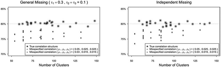
Empirical power under misspecified correlation structure.

References

- 1.Rutterford C, Copas A and Eldridge S. Methods for sample size determination in cluster randomized trials. Int J Epidemiol 2015; 44(3): 1051–1067. [DOI] [PMC free article] [PubMed] [Google Scholar]
- 2.Preisser JS, Young ML, Zaccaro DJ, et al. An integrated population-averaged approach to the design, analysis and sample size determination of cluster-unit trials. Stat Med 2003; 22(8): 1235–1254. [DOI] [PubMed] [Google Scholar]
- 3.Obuchowski NA. On the comparison of correlated proportions for clustered data. Stat Med 1998; 17(13):1495–1507. [DOI] [PubMed] [Google Scholar]
- 4.Fiero MH, Huang S, Oren E, et al. Statistical analysis and handling of missing data in cluster randomized trials: a systematic review. Trials 2016; 17(1): 72. [DOI] [PMC free article] [PubMed] [Google Scholar]
- 5.Turner EL, Li F, Gallis JA, et al. Review of recent methodological developments in group-randomized trials: part 1-design. Am J Public Health 2017; 107(6): 907–915. [DOI] [PMC free article] [PubMed] [Google Scholar]
- 6.Taljaard M, Donner A and Klar N. Accounting for expected attrition in the planning of community intervention trials. Stat Med 2007; 26(13): 2615–2628. [DOI] [PubMed] [Google Scholar]
- 7.Wood DA, Kotseva K, Connolly S, et al. Nurse-coordinated multidisciplinary, family-based cardiovascular disease prevention programme (EUROACTION) for patients with coronary heart disease and asymptomatic individuals at high risk of cardiovascular disease: a paired, cluster-randomised controlled trial. Lancet 2008; 371(9629): 1999–2012. [DOI] [PubMed] [Google Scholar]
- 8.Weaver MR, Crozier I, Eleku S, et al. Capacity-building and clinical competence in infectious disease in Uganda: a mixed-design study with pre/post and cluster-randomized trial components. PLoS One 2012; 7(12): e51319. [DOI] [PMC free article] [PubMed] [Google Scholar]
- 9.Boult C, Leff B, Boyd CM, et al. A matched-pair cluster-randomized trial of guided care for high-risk older patients. J Gen Intern Med 2013; 28(5): 612–621. [DOI] [PMC free article] [PubMed] [Google Scholar]
- 10.Bavarian N, Lewis KM, DuBois DL, et al. Using social-emotional and character development to improve academic outcomes: A matched-pair, cluster-randomized controlled trial in low-income, urban schools. J Sch Health 2013; 83(11): 771–779. [DOI] [PMC free article] [PubMed] [Google Scholar]
- 11.Roy A, Bhaumik DK, Aryal S, et al. Sample size determination for hierarchical longitudinal designs with differential attrition rates. Biometrics 2007; 63(3): 699–707. [DOI] [PubMed] [Google Scholar]
- 12.Liu G and Liang KY. Sample size calculations for studies with correlated observations. Biometrics 1997; 53(3): 937–947. [PubMed] [Google Scholar]
- 13.Zhang S and Ahn C. Sample size calculation for time-averaged differences in the presence of missing data. Contemp Clin Trials 2012; 33(3): 550–556. [DOI] [PMC free article] [PubMed] [Google Scholar]
- 14.Zhu H, Zhang S and Ahn C. Sample size considerations for split-mouth design. Stat Methods Med Res 2017; 26(6): 2543–2551. [DOI] [PMC free article] [PubMed] [Google Scholar]
- 15.Zhang S, Cao J and Ahn C. Sample size calculation for before-after experiments with partially overlapping cohorts. Contemp Clin Trials 2018; 64: 274–280. [DOI] [PMC free article] [PubMed] [Google Scholar]
- 16.Zhu H, Xu X and Ahn C. Sample size considerations for paired experimental design with incomplete observations of continuous outcomes. Stat Methods Med Res 2019; 28(2): 589–598. [DOI] [PubMed] [Google Scholar]
- 17.Liang KY and Zeger SL. Longitudinal data analysis using generalized linear models. Biometrika 1986; 73(1): 13–22. [Google Scholar]
- 18.Murray DM. Design and Analysis of Group-Randomized Trials. New York, NY: Oxford University Press, 1998. [Google Scholar]
- 19.Li P and Redden DT. Small sample performance of bias-corrected sandwich estimators for cluster-randomized trials with binary outcomes. Stat Med 2015; 24(2): 281–296. [DOI] [PMC free article] [PubMed] [Google Scholar]
- 20.Preisser JS, Lu B and Qaqish BF. Finite sample adjustments in estimating equations and covariance estimators for intracluster correlations. Stat Med 2008; 27(27): 5764–5785. [DOI] [PubMed] [Google Scholar]
- 21.Rubin DB. Inference and missing data. Biometrika 1976; 63(3): 581–592. [Google Scholar]
- 22.Yin G Clinical trial design: Bayesian and frequentist adaptive methods. Hoboken, NJ: John Wiley & Sons, 2012. [Google Scholar]
- 23.Turner RM, Omar RZ and Thompson SG. Bayesian methods of analysis for cluster randomized trials with binary outcome data. Stat Med 2001; 20: 453–472. [DOI] [PubMed] [Google Scholar]
- 24.Kauermann G and Carroll RJ. A note on the efficiency of sandwich covariance matrix estimation. J Am Statist Assoc 2001; 96(456): 1387–1396. [Google Scholar]
- 25.Mancl LA and DeRouen TA. A covariance estimator for GEE with improved small-sample properties. Biometrics 2001; 57(1): 126–134. [DOI] [PubMed] [Google Scholar]
- 26.Andrade S, Lachat C, Ochoa-Aviles A, et al. A school-based intervention improves physical fitness in Ecuadorian adolescents: a cluster-randomized controlled trial. Int J Behav Nutr Phys Act 2014; 11(1): 153. [DOI] [PMC free article] [PubMed] [Google Scholar]
- 27.Robins JM, Rotnitzky A and Zhao LP. Analysis of semiparametric regression-models for repeated outcomes in the presence of missing data. J Am Stat Assoc 1995; 90: 106–121. [Google Scholar]
- 28.Graybill FA. Matrices with Applications in Statistics. Belmont, CA: Brooks/Cole, 1983. [Google Scholar]