Analysis on the spatio-temporal characteristics of COVID-19 in mainland China

Abstract

COVID-19 has brought many unfavorable effects on humankind and taken away many lives. Only by understanding it more profoundly and comprehensively can it be soundly defeated. This paper is dedicated to studying the spatial-temporal characteristics of the epidemic development at the provincial-level in mainland China and the civic-level in Hubei Province. Moreover, a correlation analysis on the possible factors that cause the spatial differences in the epidemic's degree is conducted. After completing these works, three different methods are adopted to fit the daily-change tendencies of the number of confirmed cases in mainland China and Hubei Province. The three methods are the Logical Growth Model (LGM), Polynomial fitting, and Fully Connected Neural Network (FCNN). The analysis results on the spatial-temporal differences and their influencing factors show that: (1) The Chinese government has contained the domestic epidemic in early March 2020, indicating that the number of newly diagnosed cases has almost zero increase since then. (2) Throughout the entire mainland of China, effective manual intervention measures such as community isolation and urban isolation have significantly weakened the influence of the subconscious factors that may impact the spatial differences of the epidemic. (3) The classification results based on the number of confirmed cases also prove the effectiveness of the isolation measures adopted by the governments at all levels in China from another aspect. It is reflected in the small monthly grade changes (even no change) in the provinces of mainland China and the cities in Hubei Province during the study period. Based on the experimental results of curve-fitting and considering the time cost and goodness of fit comprehensively, the Polynomial(Degree = 18) model is recommended in this paper for fitting the daily-change tendency of the number of confirmed cases.

1. Introduction

The coronavirus disease 2019 (COVID- 19) has spread worldwide. The confirmed cases have successively appeared in more than 200 countries. COVID-19 affects people's daily lives and the social economy's operation and makes many people lose their lives. It is the common enemy of all humankind. As the first country that reports COVID-19 to the United Nations and society, the Chinese government and its people have made significant contributions to the fight against COVID-19. The Chinese government has been announcing worldwide the number of confirmed cases, new cases, died cases, cured cases, and suspected cases, as well as the response measures it has taken, nearly in real-time (N. H. C. of the People's Republic of China, 2021). These measures enable people to know the development and change of COVID-19 in China and provide decision supports and experience references for other countries to cope with COVID-19. Also, due to the openness of the data, many researchers can carry out relevant researches on COVID-19.

In this paper, the data about the number of confirmed cases in China are obtained from the website of the National Health Commission of the People's Republic of China (N. H. C. of the People's Republic of China, 2021) to analyze the spatial-temporal characteristics of the epidemic situation in China during the period from January 16, 2020, to July 31, 2020. After that, the possible impact indicators that cause regional differences in the number of confirmed cases are explored. Then the curve-fitting on the daily-change tendency of the number of confirmed cases is carried on. This paper aims to understand the spatio-temporal differences of the epidemic at both the provincial-level in mainland China and the civic-level in Hubei Province. It also proves to a certain extent that the epidemic prevention measures adopted by the governments at all levels in mainland China are effective.

2. Related work

Since the outbreak of COVID-19, researchers worldwide have been carrying out a lot of research works on it. These researches can be mainly divided into the following six categories: (1) to study the impact of COVID-19 on human physical and mental health from a biomedical perspective (Tsamakis et al., 2020, Xiong et al., 2020, Pascoal et al., 2021); (2) to study the impact of COVID-19 on human production, life, and social and economic development from a sociological perspective (Takyi and Bentum-Ennin, 2020, Qian et al., 2021, Shang et al., 2021, Beiderbeck et al., 2021, Jiang et al., 2021); (3) to creatively propose new mathematical models or revise some existing models based on relevant data for predicting and analyzing the development of the epidemic in a specific area (Vianello et al., 2021, Willis et al., 2021, Mun and Geng, 2021, Al-qaness et al., 2021, Manenti et al., 2020, Hu et al., 2020, Cao et al., 2020, Mojjada et al., 2020, Yang et al., 2020); (4) to analyze the spatial-temporal characteristics of the epidemic in a specific area (Lv and Cheng, 2020, Feng et al., 2020); (5) to explore related factors which may affect the development of the epidemic (Hu et al., 2021); (6) to evaluate the effects of different epidemic prevention measures (Leung et al., 2020, Hasnain et al., 2020). In terms of the research purpose and content, the third, the fourth, and the fifth categories are more relevant to the work carried out in this paper.

To complement medical actions to contrast the spread of infections such as COVID-19, Vianello et al. (2021) have carried out some significant works. They pointed out that tracing confirmed cases and predicting the local contagion dynamics through early indicators are crucial measures to a successful fight against emerging infectious diseases (EID). Then, based on the publicly available raw data on the spread of SARS-CoV-2 sourced from the database of the Italian Civil Protection Department, they proposed a model-free framework and applied Early Warning Detection Systems (EWDS) techniques to detect changes in the territorial spread of infections in the very early stages of onset. Further, two distinct EWDS approaches were adapted and applied to the current SARS-CoV-2 outbreak by them. Their experimental results show that the approaches can promptly generate warning signals and detect the onset of an epidemic at early surveillance stages even if working on the limited daily available, open-source data. Willis et al. (2021) aimed to demonstrate the effectiveness of using parameter regression methods to calibrate a SIRD model for COVID-19. The effective reproduction number response to NPIs (non-pharmaceutical interventions) is non-linear and variable in response rates, magnitude, and direction. During the experiments, they exploited the sophisticated parameter regression functionality of a commercial chemical engineering simulator with piecewise continuous integration, event and discontinuity management. Their main contribution is developing a strategy for calibrating and validating a model rather than presenting a fully optimized model or attempting to predict the future course of the COVID-19 pandemic. Considering that the assumption of the classic rate law central to the SIR compartmental models is not always true, Mun and Geng (2021) designed a modified mathematical model for non-first-order kinetics. Especially, they discuss two coefficients associated with the modified epidemic model: transmission rate constant k and transmission reaction order n. The experiments based on the observed data from 127 countries during the initial phase of the COVID-19 pandemic have validated their model's superiority because it can remove an implicit assumption on reaction order in the classic SIR compartmental models to be more general, flexible, and accurate. Al-qaness et al. (2021) propose a new short-term forecasting model using an enhanced version of the adaptive neuro-fuzzy inference system (ANFIS). An improved marine predators algorithm (MPA), called chaotic MPA (CMPA), is applied to enhance the ANFIS and avoid its shortcomings. Manenti et al. (2020) pointed out that there are analogies between the pandemic infection of SARS-CoV-2 and the behavior of chemical reactors. Based on this point, they modeled the virus spreading as a batch (i.e., an intrinsically dynamic chemical reactor), providing a phenomenological interpretation of data to monitor and predict the time evolution of the spreading process. Thanks to their studies, in reaction engineering terms, it is possible to distinguish four infection stages of epidemics/pandemics: the starting stage (infection outbreak), the early stage (infection transmission), the mature stage (infection mitigation), and the final stage (infection extinction). By the time they published this literature, the Hubei province has been in the final stage, while South Korea has just entered the mature stage. They claimed that each phase's kinetic parameters would be properly estimated once all the data and the related convergence paths are collected. Especially, the model is progressively improving the predictions every day to support all the countries affected by the SARS-CoV-2 pandemic to make decisions and organize supplies and human resources. Hu et al. (2020) propose a dynamic growth rate model to analyze the characteristics and trends of the global outbreak of COVID-19. The model is derived based on the ordinary differential equation for infectious diseases, and its generality was tested by using the epidemic data of COVID-19 in China. They utilize the model to predict the inflection points of countries facing serious outbreaks and forecast their future trends. Cao et al. (2020) established a COVID-19 SEIR transmission dynamics model, which took transmission ability in the latent period into consideration. Based on the epidemic data of Hubei province from January 23, 2020, to February 24, 2020, they fitted the parameters of the newly established modified SEIR model. Mojjada et al. (2020) commit to demonstrating the ability to predict the number of individuals affected by the COVID-19 as a potential threat to human beings by Machine Learning (ML) modeling. Their work shows that the Linear Regression (LR) effectively predicts new corona cases, death numbers, and recovery. Yang et al. (2020) use a modified susceptible-exposed-infected-removed (SEIR) epidemiological model that incorporates the domestic migration data before and after January 23 and the most recent COVID-19 epidemiological data to predict the epidemic progression. Further, they corroborate their model prediction using a machine-learning artificial intelligence (AI) approach trained on the 2003 SARS coronavirus outbreak data. Lv and Cheng (2020) use Crystal Ball and GIS software to explore the spatial and temporal characteristics of COVID-19 from January 25 to April 8 in Hubei Province, China, employing spatial autocorrelation. Feng et al. (2020) compare transmission paths, outbreaks timelines, and coping strategies of COVID-19 in China and the US based on the cumulative number of confirmed cases, number of confirmed cases per day, and cumulative number of deaths. To clarify the correlation between temperature and the COVID-19 pandemic in Hubei, Hu et al. (2021) collected daily newly confirmed COVID-19 cases and daily temperature for six cities in Hubei Province, assessed their correlations, and established regression models. They find that the government departments in areas where temperatures range between −3.9 and 16.5 °C and rise gradually must take more active measures to address the COVID-19 pandemic.

In summary, researchers have carried out a lot of researches on COVID-19 from different research perspectives. The significance and contributions of these researches must be affirmed sufficiently. They provide a basis for humans to better understand COVID-19 and its impact, thus formulating more effective prevention and even cure measures. The Chinese government has successfully controlled COVID-19 in mainland China, and its people have resumed normal production, living, learning, and work. Therefore, this paper only conducts the curve-fitting of the number of confirmed cases based on its experimental data and does not further use the obtained fitting functions to predict the number of infections in the future. Unlike the existing work of analyzing the spatio-temporal characteristics of COVID-19 in specific areas, this paper explores the spatio-temporal characteristics of the epidemic situation at two different levels (provincial-level and civic-level) and tries to find out the correlation between the characteristics got at the two different levels. In addition, unlike only analyzing the correlation between the change of the epidemic situation and a specific factor (such as temperature), this paper explores the correlations among the spatio-temporal differences of the epidemic situation and the factors that people subconsciously think are related.

3. Data and methods

The fundamental experimental data in this paper is the number of confirmed cases in China. The data of each province in China can be obtained from the website of the National Health Commission of the People's Republic of China (N. H. C. of the People's Republic of China, 2021). Similarly, the data of each city in Hubei Province can be obtained from the website of the Health Commission of Hubei Province (H. C. of Hubei Province, 2021). The data about the possible indicators (Table 1 ), which may impact the number of confirmed cases in different regions, are collected from the statistical yearbooks of the corresponding provinces, cities, and the whole country. These statistical yearbooks were released in late November 2020. All kinds of statistical data in these yearbooks are cumulative values rather than real-time values.

Table 1.

Eighteen indicators selected for correlation analysis.

Population related indicators	Economy related indicators	Gathering places related indicators
Total population size	Gross Domestic Product	Number of legal entities
Number of permanent residents	Production value of primary industry	Number of medical and health institutions
Number of employees at the end of the period	Production value of secondary industry	Number of industrial enterprises
Number of students at the end of 2019	Production value of the tertiary industry	Number of schools
Passenger traffic volume	Per capita consumption expenditure of urban residents	Total number of medical institutions, enterprises, and schools
Passenger traffic turnover	Per capita consumption expenditure of rural residents
Permanent population density

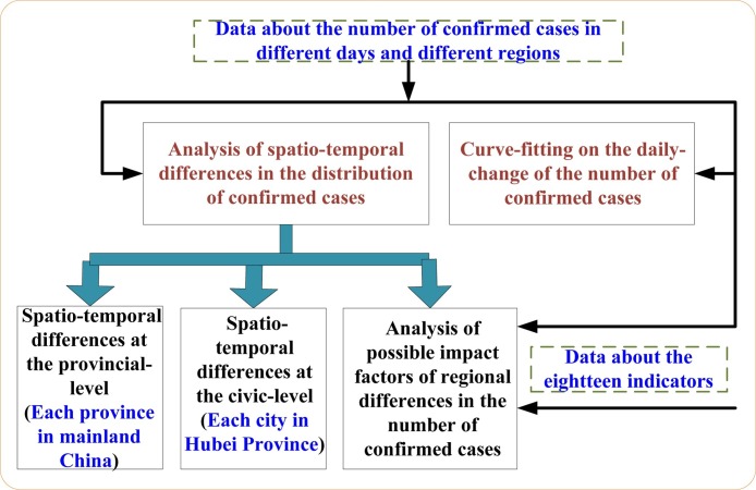
The usage of the experimental data and the research contents of this paper are shown in Fig. 1 .

Fig. 1.

Usage of the data and research contents.

As shown in Fig. 1, the spatial-temporal differences in the number of confirmed cases at the provincial-level and civic-level are analyzed. Besides that, the curve-fitting on the daily-change tendencies of the number of confirmed cases in mainland China and Hubei Province are performed.

3.1. Classification and evaluation

The Natural Breaks method is adopted to conduct the classification work to discover and compare the distribution differences of the number of confirmed cases in different regions more intuitively. The Coefficient of Variation (CV) is used for evaluating the changes in the level of different regions in different months.

3.1.1. Natural Breaks method

The Natural Breaks method (JGF, 1967) is a statistical classification method based on the numerical statistical distribution. It can maximize the differences among different classes.

There are some natural turning points and characteristic points in any statistical series. These points can be used to divide the research objects into groups with similar properties. Therefore, the breakpoints themselves are good boundaries for classification. To find the breakpoints, it needs to calculate the value of GVF (Goodness of Variance Fit) according to Eq. (1).

$$\begin{array}{c}\mathrm{SDCM}=\sum _{j=1}^k\frac{1}{N_j}\sum _{i=1}^{N_j}{(z_{\mathrm{ij}}-{\overline{z}}_j)}^2\hfill \\ \mathrm{SDAM}=\frac{1}{N}\sum _{i=1}^N{(z_i-\overline{z})}^2\hfill \\ \mathrm{GVF}=1-\frac{\mathrm{SDMC}}{\mathrm{SDAM}}\hfill \end{array}$$ (1)

In Eq. (1), k stands for the number of categories, z _ij denotes the ith element in the jth group, and ${\overline{z}}_j$ represents the mean value of all elements in the jth group; N is the number of samples, z _i is the ith element in the sample, and $\overline{z}$ is the mean value of all samples. SDAM and SDCM stand for the Sum of squared Deviations from the Array Mean, and the Sum of squared Deviations about Class Mean, respectively. Obviously, SDAM is a constant, while SDCM is related to the classification number k, and GVF  ∈ [0, 1].

GVF can be used to compare the classification effects of different methods under the same number of classes and compare that of the same method under different classification numbers. Usually, the classification result corresponding to the maximum GVF value will be selected. Suppose that, at this time, the statistical series is divided into $\{\{z_{11},z_{12},\dots ,z_{1n_1}\},\{z_{21},z_{22},\dots ,z_{2n_2}\},\dots ,\{z_{(k-1)1},z_{(k-1)2},\dots ,z_{(k-1)n_{k-1}}\},\{z_{k1},z_{k2},\dots ,z_{{\mathrm{kn}}_k}\}\}$, where n _i is the size of the ith category and ${\sum }_{i=1}^k=N$. Then, the elements $z_{1n_1},z_{2n_2},\dots ,z_{(k-1)n_{k-1}}$ can be viewed as the natural breakpoints of the original series. It should be noted that the index of each element in the classification result is exactly the same as that in the original series.

3.1.2. Coefficient of Variation (CV)

The CV is a statistic that measures the variation degree of each observation in the data. It has no dimensions, making it possible to compare the dispersion degree of two data sets objectively. Like range, standard deviation, and variance, CV is an absolute value reflecting the dispersion degree of data. The magnitude of its value is affected by the dispersion degree and the average level of the variable. Eq. (2) can be used to calculate the value of CV.

$$\mathrm{CV}=\frac{\sqrt{{\sum }_{i=1}^n{(x_i-\overline{x})}^2}}{n\overline{x}}$$ (2)

In Eq. (2), x _i  ∈  X where X is the values of a specific property of an object in different situations. $\overline{x}$ is the mean of all the elements in the set X, while n is the number of elements in X. In general, the higher the average level of the variable value, the larger the measurement value of its dispersion. In statistical analysis, if the CV value of a group of data is greater than 15% then the data may be considered as abnormal.

3.2. Curve-fitting method

In this paper, three kinds of methods are adopted to conduct the curve-fitting. They are Logistic Growth Model (LGM), Polynomial fitting method, and Fully Connected Neural Network (FCNN), respectively. Further, the goodness of fit (R ²) index is used to evaluate the fitting effect quantitatively.

3.2.1. Logistic Growth Model (LGM)

LGM is often used to model data from population, biological population growth, economic indicators, and other fields. Unlike the exponential model, LGM will reduce the growth rate when it grows to a particular stage until it reaches a specific maximum value. In addition, it is widely used in complex system dynamics, such as growth limits, social competition, and macroeconomic forecasting. During SARS in 2003, some scholars used LGM to make predictions (Huang et al., 2003, Ang, 2004). The mathematical expression of LGM is shown as Eq. (3).

$$y=\frac{k}{1+{\mathrm{e}}^{-a(x-b)}}$$ (3)

In Eq. (3), k is the upper limit of population size, while the value of a reflects the growth rate. b is the inflection point where the ascent speed reaches the highest and then slows down.

3.2.2. Polynomial fitting

Suppose the polynomial obtained by fitting is f(x) =  p ₀ x ⁿ  +  p ₁ x ⁿ⁻¹  +  p ₂ x ⁿ⁻²  +  p ₃ x ⁿ⁻³  + ⋯ +  p _n, the difference between the fitting function and the actual result could be defined as $\mathrm{loss}={\sum }_{i=1}^n{(y_i-f(x_i))}^2$.

The purpose of the polynomial fitting is to find a set of {p ₀, p ₁, …, p _n} to make the fitting result as consistent with the actual sample data as possible. It also means minimizing the value of loss. The {p ₀, p ₁, …, p _n} is the coefficients of each term in the polynomial f.

3.2.3. Fully Connected Neural Network (FCNN)

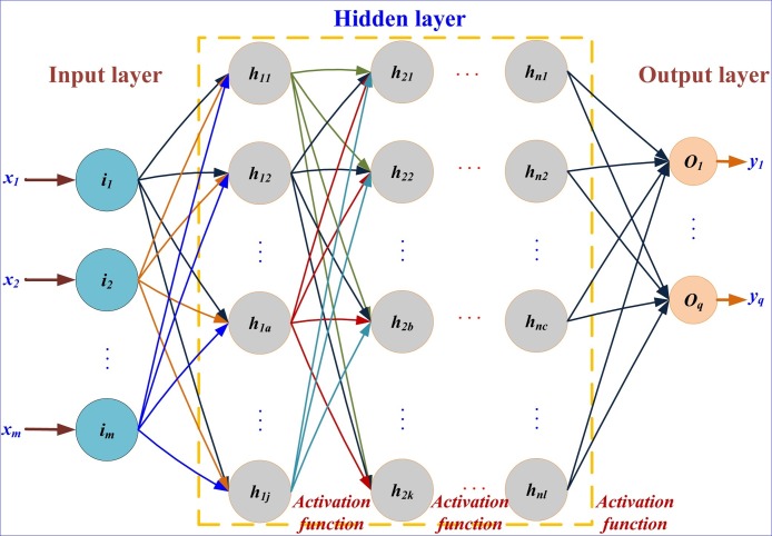
FCNN is a kind of neural network with one input layer, one output layer, and m (m  ≥ 1) hidden layers. The neurons in the same layer are not connected with each other, while each neuron in the previous layer is connected with all neurons in the next layer. The structure of FCNN is shown in Fig. 2 .

Fig. 2.

Fully Connected Neural Network.

In FCNN, all input information received by the neuron in the previous hidden layer is processed by a linear integration and an activation function. The processing result will be used as the input of the neurons connected to it in the next hidden layer. In the same way, the information received by the neuron in the last hidden layer undergoes the same processing as the input of the neuron connected to it in the output layer. Some commonly used activation functions are shown in Table 2 .

Table 2.

Activation functions.

Function	Mathematical expression
Sigmoid	$f(z)=\frac{1}{1+{\mathrm{e}}^{-z}}$
tanh	$\tanh (x)=\frac{{\mathrm{e}}^x-{\mathrm{e}}^{-x}}{{\mathrm{e}}^x+{\mathrm{e}}^{-x}}$
ReLU	Relu = max(0, x)
Leaky ReLU(PReLU)	$f(x)=\left\{\begin{array}{cc}\hfill x\hfill & \hfill \mathrm{x}\ge 0\hfill \\ \hfill \alpha x\hfill & \hfill \mathrm{x}<0\hfill \end{array}\right)$
ELU	$f(x)=\left\{\begin{array}{cc}\hfill x\hfill & \hfill \mathrm{x}\ge 0\hfill \\ \hfill \alpha ({\mathrm{e}}^x-1)\hfill & \hfill \mathrm{x}<0\hfill \end{array}\right)$
Softsign	$f(x)=\frac{x}{1+|x|}$
SoftPlus	f(x) = ln(1 + ex)
Maxout	$f(x)=\max (w_1^{T}x+b_1,w_2^{T}x+b_2,\dots ,w_n^{T}x+b_n)$

If m  > 2, the FCNN can be considered as a DNN (Deep Neural Networks). The nonlinear fitting capability of DNN is powerful and can fit almost any function.

3.2.4. Fitting capacity estimate (R²)

The goodness of fit refers to how well the regression line fits the observations. The statistic that measures the goodness of fit is the coefficient of determination (R ²  ∈ [0, 1])), according to Eq. (4).

$$R^2=1-\frac{\mathrm{RSS}}{\mathrm{TSS}}=1-\frac{{\sum }_{i=1}^m{(\widehat{y_i}-y_i)}^2}{{\sum }_{i=1}^m{(y_i-\overline{y})}^2}$$ (4)

Where RSS is the abbreviation of ‘Residual Sum of Squares’ while TSS is that of ‘Total Sum of Squares’. m is the number of samples, while y _i and $\widehat{y_i}$ are the true output and predicted output of the ith sample, respectively. $\overline{y}$ is the mean value of all y _i(i  = 1, 2, …, m). The larger the value of R ², the better the fitting effect.

4. Experiments and analysis

This section first analyzes COVID-19's spatial-temporal characteristics in China from January 16, 2020, to July 31, 2020, is conducted. Then, the possible impact indicators that may cause these spatial-temporal differences are explored. Finally, the fitting effects of the daily-change tendency of the number of confirmed cases obtained using the three kinds of methods are compared and evaluated.

4.1. Temporal differences analysis

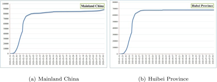
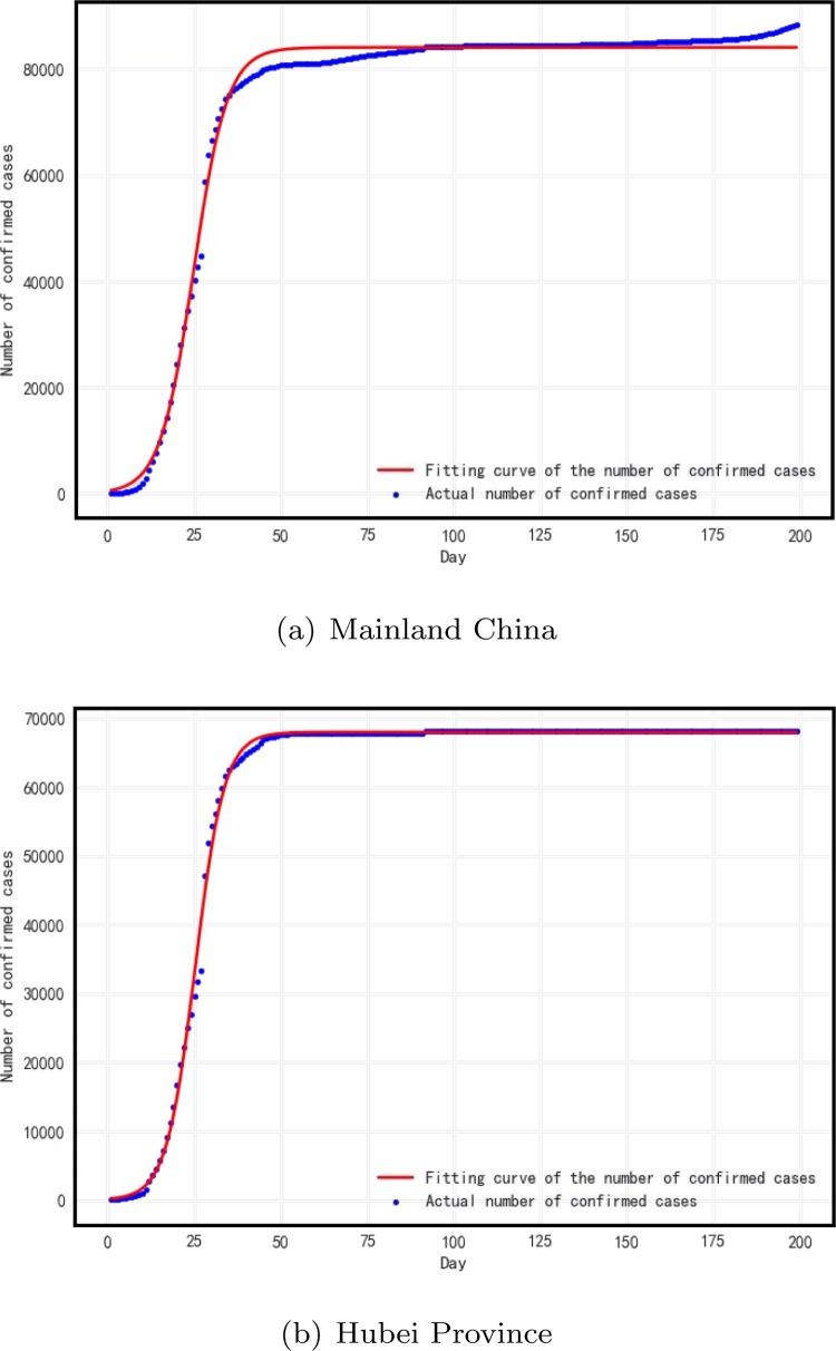
The actual change curves of the number of confirmed cases in mainland China and Hubei Province over time are shown in Fig. 3 (a) and (b), respectively.

Fig. 3.

The daily-change tendency of the number of confirmed cases.

As the first city in China to report and appear the confirmed cases, Wuhan city has taken many effective measures to control the spread of the epidemic, such as sealing off the city from all outside contact. These effective isolation and prevention measures make the epidemic development and change tendency of Wuhan City directly determine that of Hubei Province and the entire country. The most direct evidence for this conclusion is that the correlation coefficient of the two change curves in Fig. 3(a) and (b) is approximately 99.78%.

The epidemic variations during the study period of this paper can be divided into three stages.

• *Early-stage of the epidemic (before January 22, 2020): During this period, the local government did not do any intervention, and the people lived normally. The number of infected people is small, so the infection rate is much lower than that in the outbreak period. In addition, as the people know very little about the virus, both the confirmed rate and admission rate of hospitals at this stage are lower.
• *Outbreak period (from January 23, 2020, to February 12, 2020): The people have a certain understanding of the virus, but the infection rate has risen to the highest because of the increase in the number of infected people. At this stage, the local government stepped up intervention to control population movement. Especially, Wuhan city sealed off itself from all outside contact to limit the spread of the epidemic on January 23, 2020. Besides that, Huoshenshan, Leishenshan, and Fangcang shelter hospitals were established to treat patients successively, increasing the confirmed rate and admission rate. Huoshenshan hospital and Leishenshan hospital were put into operation on February 3, 2020, and February 6, 2020. Under the unified command and dispatch of the Chinese government, the lower-level governments nationwide supported Hubei Province actively. They sent the residents’ daily necessities to Hubei Province and, more importantly, provided them numerous medical workers and medical supplies.
• *Stable period (after February 13, 2020): During this period, the number of confirmed cases first rose sharply, then the growth slowed and gradually stagnated. Something that needs to be explained is that the sharp increase is not caused by the out-of-control of the epidemic but the revision of the confirmed rule on February 13, 2020. Under the new rules, the data of clinical diagnosis was included.

4.2. Spatial differences analysis

This section analyzes the spatial differences among all the provinces in mainland China and all the cities of Hubei Province.

4.2.1. Spatial differences at the provincial-level

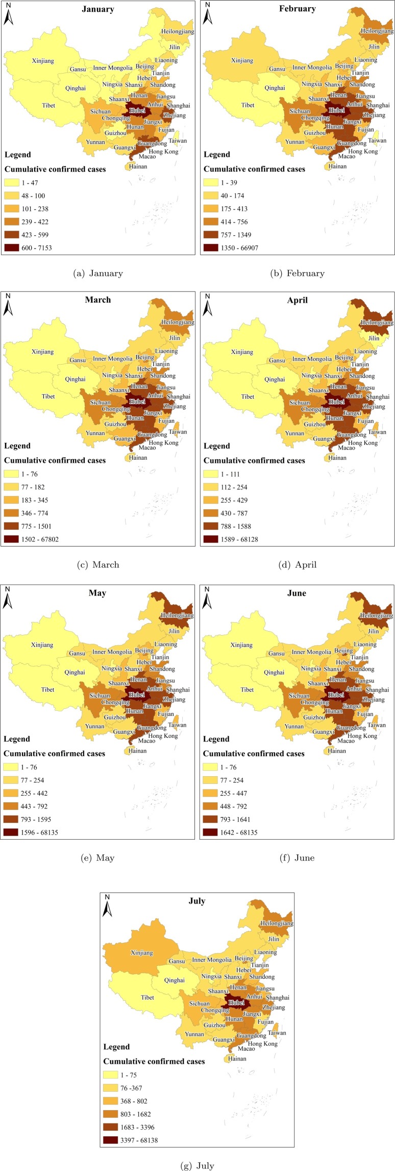
The Natural Breaks method is adopted to conduct the classification based on the number of confirmed cases of each province in mainland China at the end of each month. The results are shown in Fig. 4 .

Fig. 4.

Classification results (provinces in Mainland China).

As depicted in Fig. 4, all the provinces are divided into six levels. With the only exception represented by Wuhan, it is possible to state that the core areas of the epidemic are first mainly located in Hubei Province's direct neighboring provinces (Henan, Anhui, Zhejiang, Jiangxi, and Hunan Province) and one of its indirect neighboring provinces (Guangdong Province). Then, due to the impact of imported cases, the number of confirmed cases in Heilongjiang Province and Beijing increased significantly and became high-risk areas. To quantitatively evaluate and compare the changes in the levels of each province in different months, the variation coefficients of each province are calculated. The results are shown in Table 3 . A smaller coefficient means minor volatility.

Table 3.

Levels and variation coefficients.

The numbers (1–6) correspond to the six levels in Fig. 4.

A smaller level number means fewer confirmed cases.

According to the classification results, most provinces have less volatility in their grades, which is reflected in their small variation coefficients, and even 0. The reason for some provinces with relatively higher variation coefficients, such as Shanxi Province, Ningxia Province, Gansu Province, and Inner Mongolia, mainly due to their confirmed number happen to be on the dividing line between the nth level and the (n  + 1)th level.

4.2.2. Spatial differences at the civic-level

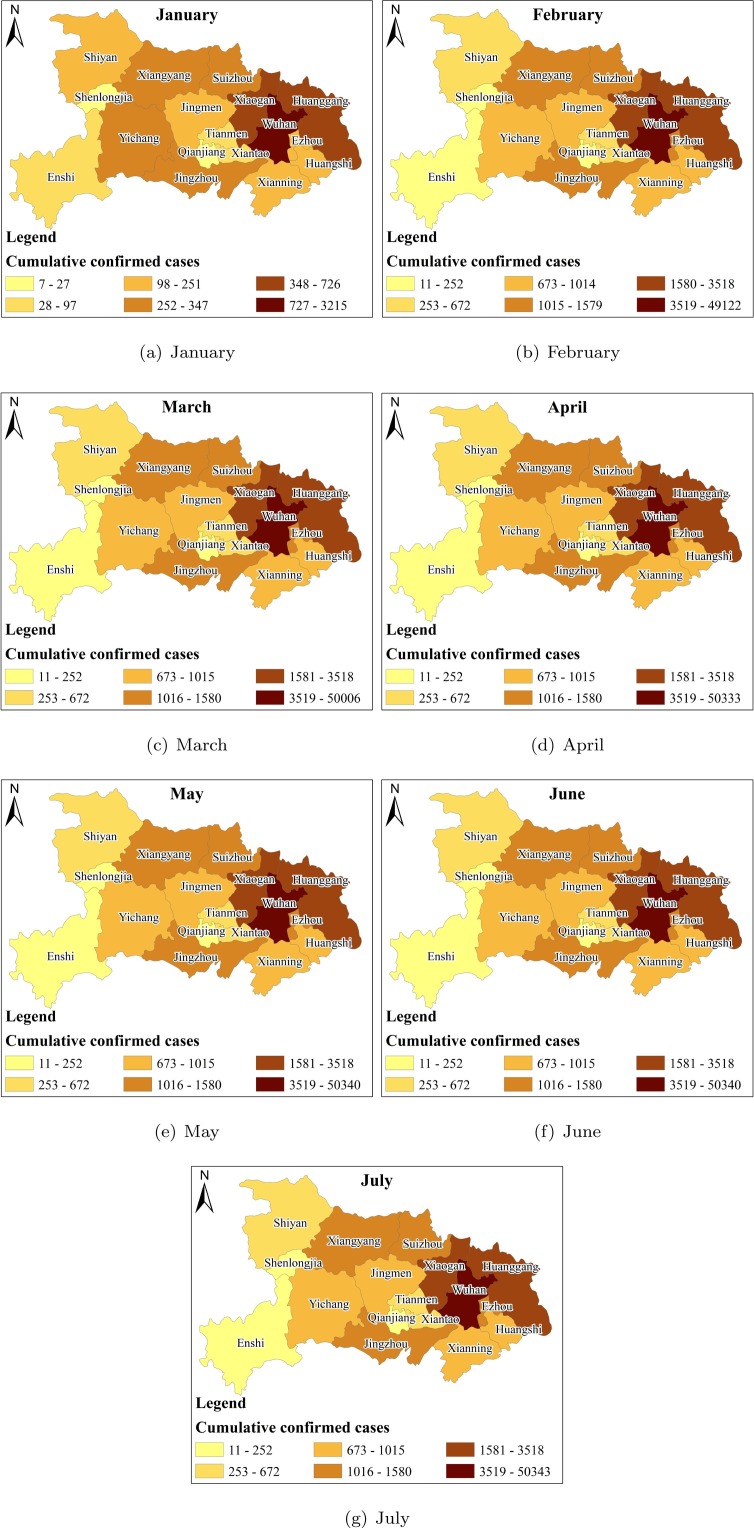
The classification results based on the number of confirmed cases of each city in Hubei Province at the end of each month are shown in Fig. 5 (a)–(g).

Fig. 5.

Classification results (cities in Hubei Province).

Geographically, the high-risk areas of the epidemic in Hubei Province are mainly located in some northern cities with Wuhan city as the center, such as Huanggang, Xiaogan, Ezhou, Suizhou, and Xiangyang, and Jingzhou city in the south.

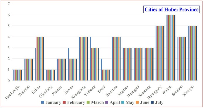
Since the number of cities in Hubei Province is small, the changes in their classification results can be displayed intuitively and clearly in the form of a picture. The classification results are directly presented in Fig. 6 . Something that needs to be explained is that the ordinate values in Fig. 6 correspond to the six levels in Fig. 5. A smaller level number means fewer confirmed cases.

Fig. 6.

Monthly classification results of cities in Hubei Province.

As seen in Fig. 6, the classification results of each city have basically not changed during the study period of this paper. It proves to a certain extent the rationality and effectiveness of the centralized isolation, community isolation, and home isolation measures adopted by local governments at all levels. These measures have effectively curbed the spread of the epidemic across regions.

4.2.3. Possible impact indicators analysis

The following eighteen possible impact indicators (Table 1) are selected for analyzing the correlation between them and the number of confirmed cases in each region as of July 31, 2020. Then, the correlation between the normalized number of confirmed cases in each region and the raw data about each indicator after normalization is analyzed. Besides that, this paper also analyzed the correlation between the ranking results based on the number of confirmed cases and that based on the raw data about each indicator. The normalization method used for the raw data is Min-Max Normalization, and the correlation analysis result is shown in Table 4 .

Table 4.

Correlation analysis result.

Indicator	Raw data (provinces in mainland China)	Ranking of raw data (provinces in mainland China)	Raw data (cities in Hubei Province)	Ranking of raw data (cities in Hubei Province)
• Total population size	0.123	.631**	.611**	.667**
• Number of permanent residents	0.113	.655**	.766**	.684**
• Number of employees at the end of 2019	0.113	.652**	.826**	.588*
• Number of students at the end of 2019	0.060	.594**	.884**	.640**
• Passenger traffic volume	0.186	.639**	0.108	.561*
• Passenger traffic turnover	0.175	.654**	0.375	.566*
• Permanent population density	−0.029	.591**	.822**	.515*
• Gross Domestic Product	0.126	.794**	.948**	.740**
• Production value of primary industry	0.203	.549**	0.314	.664**
• Production value of secondary industry	0.133	.728**	.912**	.716**
• Production value of tertiary industry	0.103	.779**	.974**	.716**
• Per capita consumption expenditure of urban residents	−0.010	0.335	.751**	0.328
• Per capita consumption expenditure of rural residents	0.108	.655**	.516*	0.306
• Number of legal entities	0.071	.735**	.934**	.613**
• Number of medical and health institutions	0.039	.469**	.726**	.561*
• Number of industrial enterprises	0.058	.717**	.775**	.789**
• Number of schools	0.044	.454*	.723**	.556*
• Total number of medical institutions, enterprises and schools	0.058	.721**	.754**	.605*

^*Correlation is significant at the 0.05 level (two-tailed).

^**Correlation is significant at the 0.01 level (two-tailed).

From Table 4 it can be argued that: (1) At the provincial-level, the correlation between the normalized data about the number of confirmed cases in each province and that of the eighteen indicators are very low and even negative. This result seems to be somewhat contrary to people's subconscious. Because people subconsciously believe that the epidemic should be more severe in areas with a larger population base, higher population density, more frequent economic activities, and more numerous public places. (2) At the provincial-level, there is a high correlation between the ranking of the number of confirmed cases and that of most indicator data, especially that of the indicators related to economic activities. (3) In terms of Hubei Province, there is a high correlation between the normalized data of the number of confirmed cases and that of the eighteen indicators and between the ranking based on the number of confirmed cases and that on most indicator data. (4) The analysis results for the cities in Hubei Province are more consistent with people's potential understanding. Generally, the objective factors that people subconsciously think may impact the severity of the epidemic may only be limited to specific regions but not universal.

4.3. Curve-fitting on the daily-change tendency of the number of confirmed cases

Logistic Growth Model (LGM), Polynomial fitting method, and Fully Connected Neural Network (FCNN) are adopted to conduct the curve-fitting. Further, to quantitatively evaluate their fitting effects, the goodness of fit (R ²) is used as an evaluation indicator.

4.3.1. Curve-fitting with LGM

The initial values of the parameters a and b are set to 0.8 and 20, respectively. As long as a  < 1 and b  ≤  n where n is the total number of records, the model will eventually converge. Given the effective quarantine measures adopted in various places after the outbreak of COVID-19, the upper limit of the number of confirmed cases is set to the total population of the local area at the end of 2019. Thus, the initial values of k are set to 59,170,000 and 1,393,444,300 for Hubei Province and mainland China, respectively. Then, the Least Square method is adopted to solve the parameters (k, a, and b) in model fitting. The results are as follows:

[k, a, b]_{Hubei_Province}  = [6.80112920e+04, 2.39021824e−01, 2.53400625e+01], R ²  = 0.998014247506507

[k, a, b]_{Mainland_China}  = [8.40794961e+04, 2.05637106e−01, 2.48323666e+01], R ²  = 0.9945165287399441

Whether seen from the fitting effect (Fig. 7 ) or the values of R ², it can be found that the fitting effect of LGM on the daily-change tendency of the number of confirmed cases in Hubei Province is better than that on mainland China.

Fig. 7.

Curve-fitting with LGM.

4.3.2. Curve-fitting with polynomial

To make this method be comparable with the LGM, the experiment in this section is devoted to obtaining the polynomial with its R ² is approximated to that of the LGM. The polynomials corresponding to the different highest coefficients are fitted, and the R ²'s values in each case are calculated. The calculation results are shown in Table 5 .

Table 5.

R² at different degrees.

Degree	$R_{\mathrm{Hubei}\_\mathrm{Province}}^2$	$R_{\mathrm{Mainland}\_\mathrm{China}}^2$
1	0.400366599788	0.452853587813
2	0.749253285945	0.772317836082
3	0.911246372103	0.927012116056
4	0.939331443350	0.952318498027
5	0.940160055628	0.952334275190
6	0.958652593897	0.964814578369
7	0.979929919807	0.982065975157
8	0.987664329504	0.991004480261
9	0.987777548338	0.991527853218
10	0.989759781030	0.992636504842
11	0.993418679382	0.995346399411
12	0.995350466059	0.997015114885
13	0.995516142766	0.997197513532
14	0.995747335406	0.997295947490
15	0.996567222552	0.997746582029
16	0.997154468451	0.998111106709
17	0.997216150758	0.998166782229
18	0.997301524355	0.998211877454
19	0.997266019958	0.998194104144

Bold values indicate value decreases.

From Table 5 it can be found that the R ²'s value always increases when Degree  ≤ 18, and then decreases slightly. Although the $R_{\mathrm{Mainland}\_\mathrm{China}}^2$'s value of Polynomial(Degree  = 11) is approximate to that obtained by the LGM, their $R_{\mathrm{Hubei}\_\mathrm{Province}}^2$'s values are quite different. After comprehensive consideration of the value of $R_{\mathrm{Mainland}\_\mathrm{China}}^2$ and $R_{\mathrm{Hubei}\_\mathrm{Province}}^2$, the ultimate value of Degree is set to 18. In this situation, the R ²'s values of Polynomial(Degree  = 18) are approximate to that obtained by the LGM. The coefficient vectors of the polynomials at this point are denoted as coff _{Hubei_Province} and coff _{Mainland_China}, respectively. Their values are shown as follow:

coff _{Hubei_Province}  = [−4.42545158e−29, 7.77937554e−26, −6.23444032e−23, 3.01223934e−20, −9.77294380e−18, 2.24263459e−15, −3.72907818e−13, 4.51451769e−11, −3.91520035e−09, 2.30452026e−07, −7.68334612e−06, −5.42396144e−06, 1.44692006e−02, −7.33550444e−01, 1.84152116e+01, −2.47610756e+02, 1.72385463e+03, −5.23546704e+03, 4.72510098e+03]

coff _{Mainland_China}  = [−3.89744755e−29, 6.80077486e−26, −5.40274975e−23, 2.58289771e−20, −8.26982005e−18, 1.86530921e−15, −3.02904962e−13, 3.53982227e−11, −2.89191283e−09, 1.49845886e−07, −2.99393226e−06, −2.00608200e−04, 1.99285238e−02, −8.21990448e−01, 1.88207932e+01, −2.38007353e+02, 1.60968786e+03, −4.84194940e+03, 4.36718838e+03]

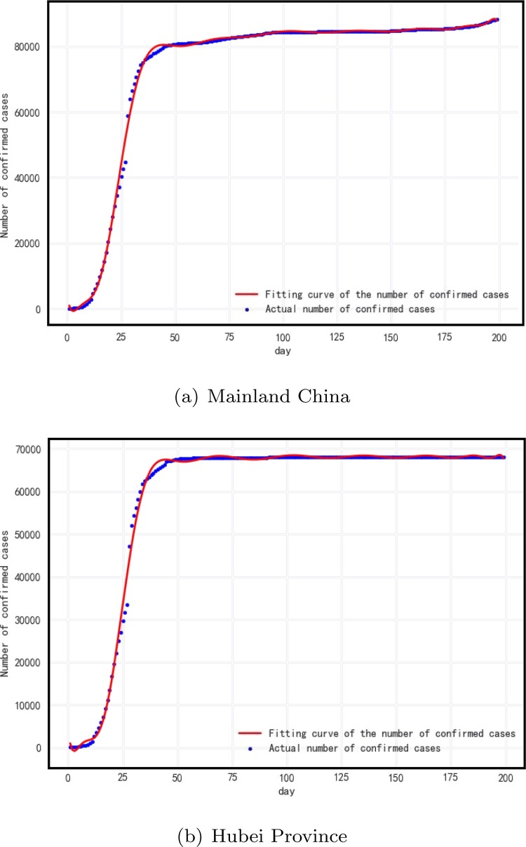
The fitting effects are shown in Fig. 8 .

Fig. 8.

Curve-fitting with polynomial (Degree = 18).

Whether seen from the fitting effect (Fig. 8) or the values of R ² (Table 5) at the same Degree, it can be found that the fitting effect of Polynomial on the daily-change tendency of the number of confirmed cases in mainland China is better than that on Hubei Province.

4.3.3. Curve-fitting with FCNN

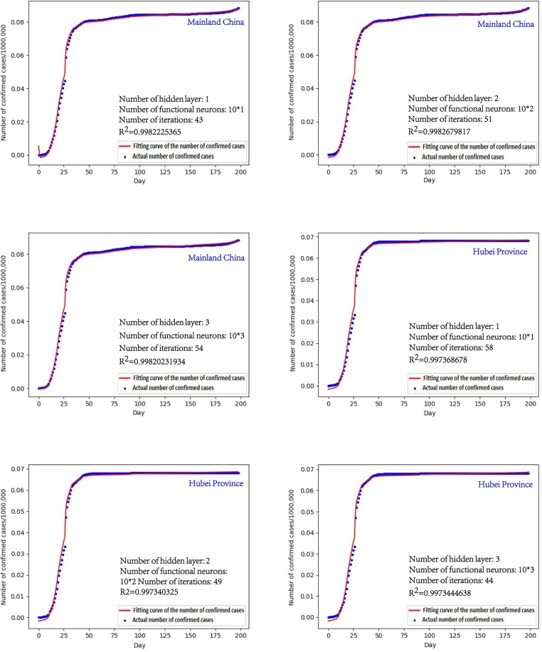
Three fully connected neural networks respectively with a single hidden layer, double hidden layers, and three hidden layers are constructed. Each hidden layer is composed of ten functional neurons. The Sigmoid function is used as the activation function between a previous hidden layer and the next hidden layer and between the last hidden layer and the output layer. Similarly, to make the different methods comparable, the value of R ² obtained by the Polynomial fitting method is used as a benchmark to determine the number of iterations of the neural networks. The fitting effects are shown in Fig. 9 .

Fig. 9.

Curve-fitting with FCNN.

The fitting results can also explain to a certain extent that the neural network can fit any function theoretically.

4.3.4. Comparison of the fitting effects of three fitting methods

The three kinds of methods on the data about mainland China and Hubei Province are run ten times. For each time, their running times and R ²'s values are recorded. Finally, the average running time and R ²’value of each method on the experimental data of this paper are calculated. The results are shown in Table 6, Table 7, Table 8, Table 9 .

Table 6.

Time costs and R²'s values of the LGM and Polynomial(Degree = 18) (Mainland China).

Round	Logistic Growth Model		Polynomial(Degree = 18)
	time cost (s)	R2	time cost (s)	R2
1	0.007000446320	0.994516528740	0.002000093460	0.998211877454
2	0.005000114441	0.994516528740	0.001000404358	0.998211877454
3	0.005000352859	0.994516528740	0.00099992752	0.998211877454
4	0.005000114441	0.994516528740	0.000999927521	0.998211877454
5	0.005000352859	0.994516528740	0.000999927521	0.998211877454
6	0.004000186920	0.994516528740	0.002000331879	0.998211877454
7	0.003999948502	0.994516528740	0.002000093460	0.998211877454
8	0.004000186920	0.994516528740	0.000999927521	0.998211877454
9	0.004000186920	0.994516528740	0.001000165939	0.998211877454
10	0.005000352859	0.994516528740	0.000999927521	0.998211877454
Average	0.004800224304	0.994516528740	0.001300072670	0.998211877454

Table 7.

Time costs and R²'s values of the FCNN with different hidden layers (Mainland China).

Round	One hidden layer			Two hidden layers			Three hidden layers
	time cost (s)	R2	iterative times	time cost (s)	R2	iterative times	time cost (s)	R2	iterative times
1	0.873049736023	0.998115977847	46	2.730156183243	0.998123776566	42	5.782330989838	0.998176211076	35
2	0.520029783249	0.998261336223	31	5.827333211899	0.998109312727	93	7.618435859680	0.998167982277	55
3	1.316075325012	0.998123336764	70	3.434196233749	0.998159477010	54	10.238585710526	0.998151921756	74
4	1.064060926437	0.998132438293	59	2.165123939514	0.998143810067	33	4.346248388290	0.998566628118	30
5	2.139122247696	0.998258420245	89	4.045231342316	0.998155315391	61	8.343477249146	0.998142517572	55
6	1.111063480377	0.998138773732	61	4.061232328415	0.998392913280	56	4.971284627914	0.998194418996	36
7	0.607034921646	0.998246457218	34	2.532144784927	0.998315240227	37	5.767330169678	0.998131084304	40
8	0.796045780182	0.998340484412	49	5.296302795410	0.998196478370	76	5.898337364197	0.998178387774	42
9	0.195010900497	0.998828843522	12	3.125178575516	0.999021452499	50	7.244414329529	0.998173984094	51
10	1.143065214157	0.998292203336	60	1.753100156784	0.997977014455	28	8.095463037491	0.998139852421	55
Average	0.976455831528	0.998273827159	51	3.496999955177	0.998259479059	53	6.830590772629	0.998202298839	47

Table 8.

Time costs and R²'s values of the LGM and Polynomial(Degree = 18) (Hubei Province).

Round	Logistic Growth Model		Polynomial(Degree = 18)
	time cost (s)	R2	time cost (s)	R2
1	0.005000114441	0.998014247507	0.004000186920	0.997301524355
2	0.004000186920	0.998014247507	0.001000165939	0.997301524355
3	0.006000280380	0.998014247507	0.001000165939	0.997301524355
4	0.006000280380	0.998014247507	0.001000165939	0.997301524355
5	0.006000518799	0.998014247507	0.001000165939	0.997301524355
6	0.005000114441	0.998014247507	0.000999927521	0.997301524355
7	0.005000114441	0.998014247507	0.000999927521	0.997301524355
8	0.003000259399	0.998014247507	0.001000165939	0.997301524355
9	0.004000425339	0.998014247507	0.000999927521	0.997301524355
10	0.004000186920	0.998014247507	0.001000165939	0.997301524355
Average	0.004800248146	0.998014247507	0.001300096512	0.997301524355

Table 9.

Time costs and R²'s values of the FCNN with different hidden layers (Hubei Province).

Round	One hidden layer			Two hidden layers			Three hidden layers
	time cost (s)	R2	iterative times	time cost (s)	R2	iterative times	time cost (s)	R2	iterative times
1	1.015058279037	0.997261077554	54	4.885279417038	0.997264302890	62	6.404366493225	0.997843871621	45
2	1.593091249466	0.997329635866	83	2.044116973877	0.997247814956	32	5.221298694611	0.997389485505	32
3	1.648094415665	0.997728075733	88	4.303246021271	0.997494009135	69	4.407252073288	0.997243617456	29
4	0.780044555664	0.997264757155	42	2.623149871826	0.997599630230	42	7.518430233002	0.997296620534	48
5	0.866049528122	0.997286638882	47	1.478084325790	0.997298756493	18	2.729156017303	0.997505670594	18
6	0.888050556183	0.997315886077	46	3.947225570679	0.997601446457	48	8.178467512131	0.997255979564	59
7	0.764043807983	0.997259507986	41	4.955283641815	0.997289058655	76	6.990399599075	0.997251829888	48
8	0.539030790329	0.997326885294	32	2.292131185532	0.997254575125	38	14.435825586319	0.997385497122	104
9	1.111063480377	0.997489166385	62	3.241185426712	0.997222436457	46	6.752386331558	0.997250216439	45
10	0.898051261902	0.997503101089	49	2.978170394897	0.997381075836	41	7.431424856186	0.997251588475	53
Average	1.010257792473	0.997376473202	54	3.274787282944	0.997365310623	47	7.006900739670	0.997367437720	48

Comparing the three methods based on the values of time  _  cost and R ² in Table 5, Table 6, Table 7, Table 8, Table 9, the following conclusions can be drawn:

• (i)A comprehensive comparison of Tables 5, 6, and 8 shows that the LGM is better than the Polynomial models with Degree  < 11 in accuracy.
• (ii)It can be concluded from Tables 6 and 8 that the LGM and the Polynomial(Degree  = 18) exhibit comparable computational performances. The two methods have time costs of the same order of magnitude and very close accuracy. More specifically, the time cost of the LGM (approximately 5 ms) is slightly higher than that of the Polynomial(Degree  = 18) (approximately 1.3 ms). In terms of accuracy, the LGM is somewhat superior to the Polynomial(Degree  = 18) in the curve-fitting for Hubei Province. However, in the curve-fitting for mainland China, the Polynomial(Degree  = 18) is marginally better. If one of the two methods has to be chosen for the fitting work, the Polynomial(Degree  = 18) is recommended in this paper, considering time cost and accuracy synthetically.
• (iii)A comprehensive comparison of Table 6, Table 7, Table 8, Table 9 shows that to achieve a similar accuracy with Polynomial(Degree  = 18), the time cost of FCNN is at least 750 to 780 times that of the Polynomial(Degree  = 18). Furthermore, the time cost of the FCNN increases with the increase of the number of hidden layers.

As mentioned in (ii), the Polynomial(Degree  = 18) is recommended to conduct the fitting work in this paper. When using the Polynomial-fitting method, it is necessary to pay attention to the under-fitting and over-fitting issues. The under-fitting issue is usually caused by too few feature dimensions or a simplistic model. It can be easily solved by adding feature items and increasing the complexity of the model. On the contrary, the over-fitting issue is usually caused by too many feature dimensions, overly complex model assumptions, too many parameters, too little training data, and too much noise. This issue will lead to instability and oscillation in the profile. To solve this issue in the Polynomial-fitting, some solutions can be considered: (1) to add training data sample; (2) to introduce regularization; (3) to use cross-validation; (4) to make a more robust data regression using sigmoidal function and assign different weights to different steady-state points; (5) to evaluate the impact of polynomial fitting as a function of function order; indeed, oscillations are not feasible once a stable condition is reached; (6) to refer to some other model calibration methods, such as (Willis et al., 2021). In terms of the fitting method and the amount of experimental data adopted in this paper, introducing regularization is preferred. The so-called ‘regularization’ introduces L1-norm or L2-norm of the parameter vector into the original loss function. The L1-norm and L2-norm are denoted as $\lambda ||w||$ and $\frac{\lambda }{2}||w|{|}^2$, respectively. Compared with the L1-norm, L2-norm is more popular. The new loss-function with introduced L2-norm can be described as ${\mathrm{loss}}_{\mathrm{new}}(w)={\sum }_{i=1}^n{(y_i-f(x_i))}^2+\frac{\lambda }{2}||w|{|}^2$. The vector $w$ is the coefficients of each term in the polynomial f. Then, the over-fitting issue can be improved by adjusting the value of λ. Lukas (2008) provides an effective way to get an appropriate value for λ.

5. Conclusions

COVID has caused many adverse effects on human production, life, and health, and even threatened human life. It is challenging to predict the trend of the COVID-19 epidemic accurately: (1) People's understanding of this virus is not comprehensive enough, and its variants continue to appear; (2) Although many prevention measures have been proven effective, it is difficult to evaluate the effectiveness of specific epidemic prevention measures quantitatively; (3) It is hard to achieve absolute isolation among individuals and among regions. In the battle against COVID-19, human beings are still in the passive defense stage. However, it should be firmly believed that COVID-19 will be soundly defeated. Since many researchers have been carrying out a lot of works on it from different perspectives. Their hard work and significant research achievements provide us with more and more professional knowledge, effective prevention measures (e.g., Leung et al., 2020), and excellent mathematical analysis or prevention models (e.g., Vianello et al., 2021).

The research results in this paper prove to a certain extent the effectiveness of the epidemic prevention measures adopted by the governments at all levels in mainland China. The measures are worth learning. It should be pointed out that it will be a more scientific and accurate way to collect the data about the relevant indicators in the same temporal interval with that about the number of the confirmed cases in this paper. However, the data about the relevant indicators are not released in real-time on the official websites of corresponding departments in mainland China. Although many of these data are recorded in real-time or regularly, only their owners or public security organizations have the right to access them. As an alternative, this paper can only get them from the statistical yearbooks.

Declaration of Competing Interest

The authors report no declarations of interest.

References

- Al-qaness M.A., Saba A.I., Elsheikh A.H., Elaziz M.A., Ibrahim R.A., Lu S., Hemedan A.A., Shanmugan S., Ewees A.A. Efficient artificial intelligence forecasting models for covid-19 outbreak in Russia and Brazil. Process Saf. Environ. Prot. 2021;149:399–409. doi: 10.1016/j.psep.2020.11.007. [DOI] [PMC free article] [PubMed] [Google Scholar]
- Ang K.C. A simple model for a sars epidemic. Teach. Math. Appl. Int J IMA. 2004;23(4):181–188. doi: 10.1093/teamat/23.4.181. [DOI] [Google Scholar]
- Beiderbeck D., Frevel N., von der Gracht H.A., Schmidt S.L., Schweitzer V.M. The impact of covid-19 on the European football ecosystem?. A delphi-based scenario analysis. Technol. Forecast. Soc. Change. 2021;165:120577. doi: 10.1016/j.techfore.2021.120577. [DOI] [Google Scholar]
- Cao S., Feng P., Shi P. Study on the epidemic development of covid-19 in hubei province by a modified seir model. J. Zhejiang Univ. (Med. Sci.) 2020;49(2):178–184. doi: 10.3785/j.issn.1008-9292.2020.02.05. [DOI] [PMC free article] [PubMed] [Google Scholar]
- Feng Z., Xiao C., Li P., You Z., Yin X., Zheng F. Comparison of spatio-temporal transmission characteristics of covid-19 and its mitigation strategies in China and the US. J. Geogr. Sci. 2020;30:1963–1984. doi: 10.1007/s11442-020-1822-8. [DOI] [Google Scholar]
- 2021. H. C. of Hubei Province. [link]http://wjw.hubei.gov.cn [Google Scholar]
- Hasnain M., Pasha M.F., Ghani I. Combined measures to control the covid-19 pandemic in Wuhan, Hubei, China: a narrative review. J. Biosaf. Biosecur. 2020;2(2):51–57. doi: 10.1016/j.jobb.2020.10.001. [DOI] [PMC free article] [PubMed] [Google Scholar]
- Hu Y., Kong J., Yang L., Wang X. A dynamic growth rate model and its application in global covid-19 epidemic analysis. Acta Math. Appl. Sin. 2020;43(2):452–467. [Google Scholar]
- Hu C., Xiao L., Zhu H., Zhu H., Liu L. Correlation between local air temperature and the covid-19 pandemic in Hubei, China. Front Public Health. 2021;(8):604870. doi: 10.3389/fpubh.2020.604870. [DOI] [PMC free article] [PubMed] [Google Scholar]
- Huang D., Guan P., Zhou B. Fitness of morbidity and discussion of epidemic characteristics of sars based on logistic models. Chin. J. Public Health. 2003;19(6):1–2. doi: 10.3321/j.issn:1001-0580.2003.06.001. [DOI] [Google Scholar]
- JGF The data model concept in statistical mapping. Int. Yearbook Cartogr. 1967;(7):186–190. [Google Scholar]
- Jiang P., Fan Y.V., Klemeš J. Impacts of covid-19 on energy demand and consumption: challenges, lessons and emerging opportunities. Appl. Energy. 2021;285:116441. doi: 10.1016/j.apenergy.2021.116441. [DOI] [PMC free article] [PubMed] [Google Scholar]
- Leung K., Wu J.T., Liu D., Leung G.M. First-wave covid-19 transmissibility and severity in China outside hubei after control measures, and second-wave scenario planning: a modelling impact assessment. Lancet. 2020;395(10233):1382–1393. doi: 10.1016/S0140-6736(20)30746-7. [DOI] [PMC free article] [PubMed] [Google Scholar]
- Lukas M.A. Strong robust generalized cross-validation for choosing the regularization parameter. Inverse Probl. 2008;24(3):034006. doi: 10.1088/0266-5611/24/3/034006. [DOI] [Google Scholar]
- Lv Z., Cheng S. Research on the temporal and spatial characteristics of the covid-19 in hubei province with the use of grystal ball and gis. J. Central Normal Univ. (Nat. Sci.) 2020;54(6):1059–1071. doi: 10.19603/j.cnki.1000-1190.2020.06.020. [DOI] [Google Scholar]
- Manenti F., Galeazzi A., Bisotti F., Prifti K., Dell’Angelo A., Di Pretoro A., Ariatti C. Analogies between sars-cov-2 infection dynamics and batch chemical reactor behavior. Chem. Eng. Sci. 2020;227:115918. doi: 10.1016/j.ces.2020.115918. [DOI] [PMC free article] [PubMed] [Google Scholar]
- Mojjada R.K., Yadav A., Prabhu A., Natarajan Y. Machine learning models for covid-19 future forecasting. Mater. Today Proc. 2020 doi: 10.1016/j.matpr.2020.10.962. [DOI] [PMC free article] [PubMed] [Google Scholar]
- Mun E.-Y., Geng F. An epidemic model for non-first-order transmission kinetics. PLOS ONE. 2021;16(3):e0247512. doi: 10.1371/journal.pone.0247512. [DOI] [PMC free article] [PubMed] [Google Scholar]
- N. H. C. of the People's Republic of China . 2021. Make Every Effort to Prevent and Control Covid-19.http://www.nhc.gov.cn/xcs/yqtb/list_gzbd.shtml [Google Scholar]
- Pascoal P.M., Carvalho J., Raposo C.F., Almeida J., Beato A.F. The impact of covid-19 on sexual health: a preliminary framework based on a qualitative study with clinical sexologists. Sex. Med. 2021;9(1):100299. doi: 10.1016/j.esxm.2020.100299. [DOI] [PMC free article] [PubMed] [Google Scholar]
- Qian X., Qiu S., Zhang G. The impact of covid-19 on housing price: evidence from China. Finance Res. Lett. 2021:101944. doi: 10.1016/j.frl.2021.101944. [DOI] [PMC free article] [PubMed] [Google Scholar]
- Shang W., Chen J., Bi H., Sui Y., Chen Y., Yu H. Impacts of covid-19 pandemic on user behaviors and environmental benefits of bike sharing: a big-data analysis. Appl. Energy. 2021;285:116429. doi: 10.1016/j.apenergy.2020.116429. [DOI] [PMC free article] [PubMed] [Google Scholar]
- Takyi P.O., Bentum-Ennin I. The impact of covid-19 on stock market performance in Africa: a bayesian structural time series approach. J. Econ. Bus. 2020:105968. doi: 10.1016/j.jeconbus.2020.105968. [DOI] [PMC free article] [PubMed] [Google Scholar]
- Tsamakis K., Rizos E., Manolis A.J., Chaidou S., Kympouropoulos S., Spartalis E., Spandidos D.A., Tsiptsios D., Triantafyllis A.S. Covid-19 pandemic and its impact on mental health of healthcare professionals. Exp. Ther. Med. 2020;19(6):3451–3453. doi: 10.3892/etm.2020.8646. [DOI] [PMC free article] [PubMed] [Google Scholar]
- Vianello C., Strozzi F., Mocellin P., Cimetta E., Fabiano B., Manenti F., Pozzi R., Maschio G. A perspective on early detection systems models for covid-19 spreading. Biochem. Biophys. Res. Commun. 2021;538(2021):244–252. doi: 10.1016/j.bbrc.2020.12.010. [DOI] [PMC free article] [PubMed] [Google Scholar]
- Willis M.J., Wright A., Bramfitt V., Díaz V.H.G. Covid-19: mechanistic model calibration subject to active and varying non-pharmaceutical interventions. Chem. Eng. Sci. 2021;231:116330. doi: 10.1016/j.ces.2020.116330. [DOI] [PMC free article] [PubMed] [Google Scholar]
- Xiong J., Lipsitz O., Nasri F., Lui L.M., Gill H., Phan L., Chen-Li D., Iacobucci M., Ho R., Majeed A., McIntyre R.S. Impact of covid-19 pandemic on mental health in the general population: a systematic review. J. Affect. Disord. 2020;277:55–64. doi: 10.1016/j.jad.2020.08.001. [DOI] [PMC free article] [PubMed] [Google Scholar]
- Yang Z., Zeng Z., Wang K., Wong S.-S., Liang W., Zanin M., Liu P., Cao X., Gao Z., Mai Z., Liang J., Liu X., Li S., Li Y., Ye F., Guan W., Yang Y., Li F., Luo S., Xie Y., Liu B., Wang Z., Zhang S., Wang Y., Zhong N., He J. Modified seir and ai prediction of the epidemics trend of covid-19 in China under public health interventions. J. Thorac. Dis. 2020;12(3):165–174. doi: 10.21037/jtd.2020.02.64. [DOI] [PMC free article] [PubMed] [Google Scholar]