CryoDRGN: Reconstruction of heterogeneous cryo-EM structures using neural networks

Abstract

Cryo-EM single-particle analysis has proven powerful in determining the structures of rigid macromolecules. However, many imaged protein complexes exhibit complex conformational and compositional heterogeneity that pose a major challenge to existing 3D reconstruction methods. Here, we present cryoDRGN, an algorithm that leverages the representation power of deep neural networks to directly reconstruct continuous distributions of 3D density maps and map per-particle heterogeneity of single particle cryo-EM datasets. Using cryoDRGN, we uncovered residual heterogeneity in high-resolution datasets of the 80S ribosome and the RAG complex, revealed a new structural state of the assembling 50S ribosome, and visualized large-scale continuous motions of a spliceosome complex. CryoDRGN contains interactive tools to visualize a dataset’s distribution of per-particle variability, generate density maps for exploratory analysis, extract particle subsets for use with other tools, and generate trajectories to visualize molecular motions. CryoDRGN is open-source software freely available at cryodrgn.csail.mit.edu.

Introduction

Proteins and their complexes are dynamic macromolecular machines that carry out the essential biological processes responsible for life. Although the mechanism of these macromolecular machines is often deduced from a static three-dimensional (3D) structure, a more complete understanding could be achieved if one could analyze the full distribution of conformations relevant to function.

Single particle cryo-electron microscopy (cryo-EM) is a rapidly maturing method for high-resolution structure determination of large macromolecular complexes^1,2. Major advances in hardware^3–5 and software^4–9 have streamlined the collection and analysis of cryo-EM datasets such that structures of rigid macromolecules can routinely be solved at near-atomic resolution^10,11. Increasingly, cryo-EM has been applied to study heterogeneous complexes as the experimental procedure is less sensitive to sample heterogeneity than other methods for structure determination^12,13. Additionally, because single particle cryo-EM can capture millions of snapshots of the molecule of interest, each carrying a unique molecule in its own conformational state¹⁴, cryo-EM holds promise in revealing the conformational landscape of dynamic macromolecular complexes. However, reconstructing ensembles of 3D volumes from such snapshots remains a major computational challenge.

Existing tools for heterogeneous reconstruction make often-limiting assumptions on the observed structural heterogeneity. Most commonly, heterogeneity is modeled as though it originates from a small number of independent, discrete states, implemented as “3D classification” or “heterogeneous refinement” in many cryo-EM software packages^15–18. However, these discrete classification approaches require specifying initial models for refinement, and because the number and nature of the underlying structural states is unknown a priori, this approach is error-prone and often results in the omission of potentially relevant structures. More critically, such discrete approaches are ill-suited for reconstructing structures undergoing continuous conformational changes.

Advanced methods for heterogeneous reconstruction seek to more closely model the continuous nature of flexible molecules. Multi-body refinement, available in RELION, models the structure as the sum of user-defined rigid bodies that are allowed to rotate relative to one another, placing structural assumptions on the observed heterogeneity¹⁹. Continuous heterogeneity has also been described using principle component analysis (PCA)-based approaches^20–22, including the recent 3D Variability Analysis (3DVA) algorithm available in cryoSPARC²³. Although the linear subspace model of these approaches can provide a summary of the overall variability within the dataset, the visualized heterogeneity contains artifacts when a molecule’s conformational deformations are poorly approximated by linear interpolations along basis volumes. In the manifold embedding approach proposed in Dashti et al.^24,25, heterogeneous structures are recovered by binning particles along the data manifold followed by traditional homogeneous reconstruction. Additional algorithms for continuous heterogeneous reconstruction have been shown on synthetic datasets^26,27.

Here, we present cryoDRGN (Deep Reconstructing Generative Networks), a method for heterogeneous cryo-EM reconstruction based on deep neural networks. We hypothesized that neural networks, which are known for their ability to model complex, nonlinear functions²⁸, could learn heterogeneous ensembles of cryo-EM density maps. We first show that our neural network representation of structure can model single density maps at high resolution, before demonstrating the full cryoDRGN framework for unsupervised heterogeneous reconstruction.

We find that cryoDRGN is a powerful and general approach for analyzing structural heterogeneity in macromolecular complexes of varying size and expected sources of heterogeneity. We show that the cryoDRGN approach can uncover residual heterogeneity in “homogeneous” datasets of the RAG1-RAG2 complex and the 80S ribosome, model large compositional changes of the assembling 50S ribosome, and continuous conformational changes of the precatalytic spliceosome. Remarkably, cryoDRGN’s unsupervised approach for representation learning can readily identify and filter impurities in the dataset and can identify rare structural states containing as few as ~1,000 particles. CryoDRGN is distributed as an open-source tool that can be easily integrated in existing pipelines and is freely available at cryodrgn.csail.mit.edu.

Results

The cryoDRGN method

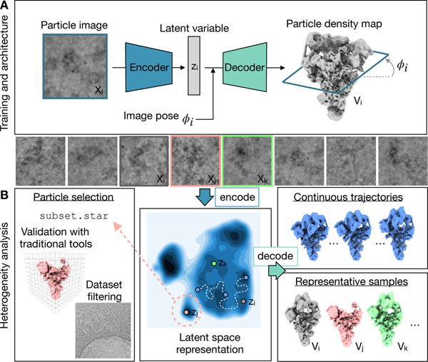
CryoDRGN performs heterogeneous reconstruction by learning a deep generative model of 3D structure from single particle cryo-EM images. The method consists of a specialized image encoder – volume decoder architecture, which learns an encoding of 2D particle images into a continuous vector space described by the latent variable z ∈ ℝⁿ (i.e. the latent space), and the concomitant reconstruction of 3D cryo-EM density maps from this latent space representation (Fig 1A). This choice of model assumes that the heterogeneous structures can be embedded within a continuous, low-dimensional manifold in the latent space, where the dimensionality of the latent space is defined by the user. The model is specified in the Fourier domain in order to relate 2D images as planar slices of the 3D volume²⁹, whose orientation is previously determined from a consensus reconstruction. The neural networks are jointly trained from random initialization using stochastic gradient descent on an objective function that seeks to maximize (a variational upper bound on) the data likelihood as in standard Variational Autoencoders (VAEs)³⁰. Additional architectural and training details of cryoDRGN are provided in the Methods section.

Figure 1. The cryoDRGN method for heterogeneous single particle cryo-EM reconstruction.

A) The cryoDRGN model consists of two neural networks structured in an image encoder-volume decoder architecture with a continuous latent variable representation of heterogeneity. During training, each particle image is encoded into the low-dimensional latent space, and then reconstructed as its corresponding model slice based on the Fourier slice theorem. Image and volume data are depicted in real space for visual clarity.

B) Once a cryoDRGN model has been trained, the full dataset of particle images is encoded into the latent space, which is visualized as a contour map here with darker regions corresponding to higher particle density (center). The decoder, which represents an ensemble of 3D density maps, can directly generate density maps from arbitrary values of the latent variable (right). The particle stack may also be filtered using the latent space representation for validation of specific structures via traditional tools or to remove impurities from the dataset (left). Example images from EMPIAR-10180³⁶.

After training, the output of cryoDRGN analysis includes: 1) per-particle latent encodings, z_i, describing the dataset’s heterogeneity; and 2) a neural network model of 3D density maps that can directly reconstruct a density map given z_i. Specifically, the encoder network encodes particle images into the continuous latent space, which allows for visualization and inspection of the particle distribution (Fig. 1B, center). The trained decoder network can then generate 3D density maps given arbitrary values of the latent variable. For example, representative structures can be generated from regions of latent space with high particle density, and continuous conformational trajectories can be reconstructed by sampling points along a trajectory through latent space (Fig. 1B, right). Notably, any cryoDRGN-generated volume can be orthogonally validated by traditional reconstruction approaches¹⁵ using nearby particles in the latent space (Fig. 1B, left). Lastly, any regions of the latent space that are enriched in impurities or imaging artifacts may be selected, and the encompassed particles filtered from subsequent analysis (Fig. 1B, left).

Neural networks can represent cryo-EM density maps

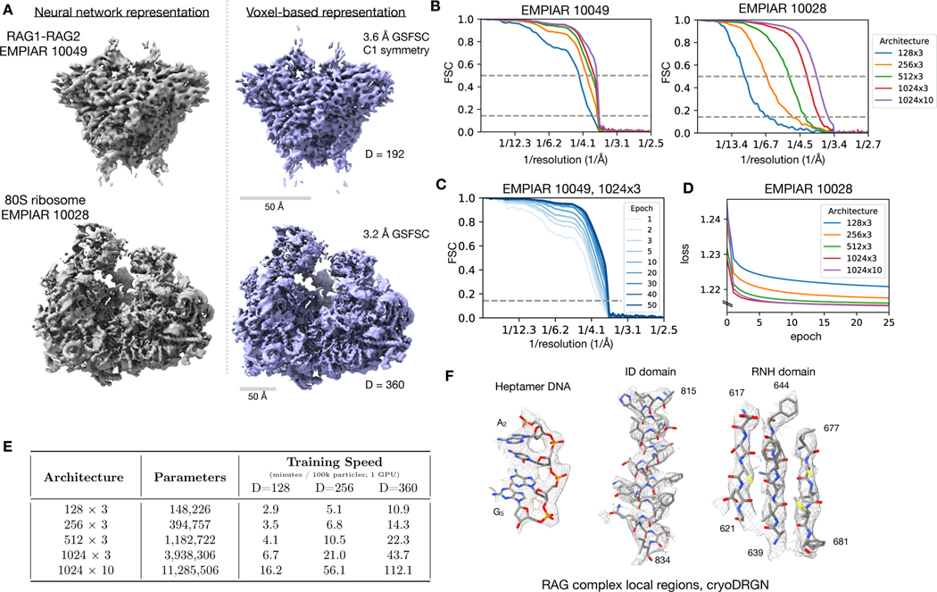
We first evaluated the cryoDRGN volume decoder in representing high resolution cryo-EM density maps. To learn the homogeneous structure of the RAG1-RAG2 signal end complex (RAG – 369 kDa)³¹ and the Plasmodium falciparum 80S ribosome (Pf80S – 4.2 MDa)³², we trained the volume decoder network with no latent variable input, using image poses obtained from C1 homogeneous refinements in cryoSPARC¹⁶ (Methods). Trained on full-resolution images, the cryoDRGN decoder produced structures that correlated with the traditional, voxel-based reconstruction (Fig. 2A) at resolutions up to 3.6 Å for RAG and 3.9 Å for Pf80S at an FSC = 0.5 threshold (Fig. 2B), demonstrating the efficacy of this neural-network based representation of 3D structure.

Figure 2). Neural network representation of cryo-EM density maps.

A) Density maps of the RAG1-RAG2 complex (EMPIAR-10049)³¹ and of the eukaryotic Pf80S ribosome (EMPIAR-10028)³² reconstructed by cryoDRGN’s decoder neural network (left) and a traditional, voxel-based reconstruction in cryoSPARC (right). The cryoDRGN volumes were generated from decoder networks with 3 hidden layers and 1024 nodes per hidden layer (denoted as 1024 × 3) trained for 25 epochs.

B) Fourier shell correlation (FSC) curves between density maps produced by the cryoDRGN decoder of varying architecture and the traditional reconstruction in (A).

C,D) Evolution of the FSC curve in (B) and the training curve over multiple epochs of cryoDRGN model training.

E) Training speed in minutes per 100k images for cryoDRGN decoder networks of different architectures on different image sizes (D, in pixels) on a single Nvidia V100 GPU.

F) Representative regions of the RAG1-RAG2 density map from cryoDRGN superimposed with the published atomic model (PDB: 3JBX).

As neural networks have a fixed capacity for representation that is constrained by their architecture, we next compared decoder architectures of different sizes to evaluate the tradeoff between representation power and training speed. We found that larger architectures, which have more trainable parameters, result in density maps that correlate with the traditionally reconstructed map at higher resolutions (Fig. 2B). The networks are trained through multiple passes through the dataset (i.e. epochs) (Fig. 2C) with lower values of the objective function (Fig. 2D) as training progressed. Notably, while the resolution of the learned structure increased with neural network size, we found that larger models were slower to train (Fig. 2E). These tradeoffs suggest that the architecture and image size should be tuned to suit the desired balance of speed and achievable resolution. Lastly, we found that the cryoDRGN architecture was capable of learning density maps at sufficiently high resolution to visualize structural features such as bulky side-chains that are consistent with our FSC-based resolution estimates (Fig. 2F).

CryoDRGN models both discrete and continuous structural heterogeneity

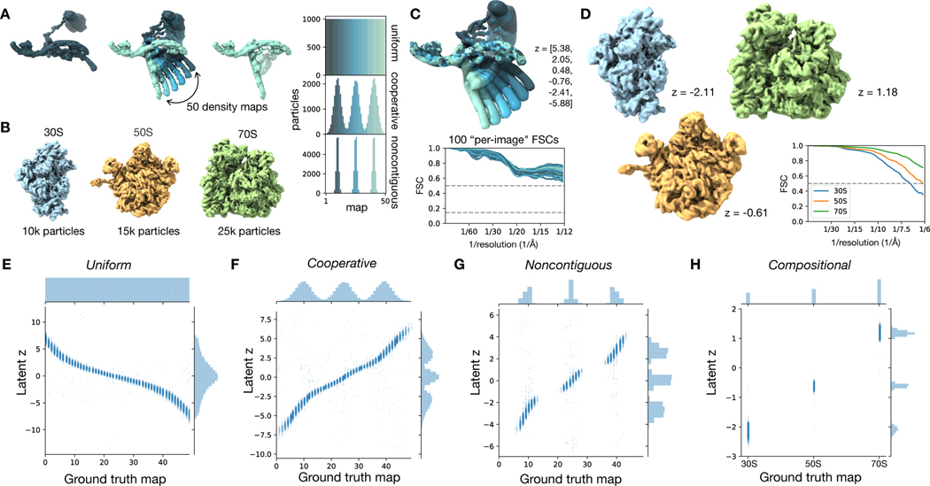
We next sought to evaluate the complete cryoDRGN framework for heterogeneous reconstruction using simulated datasets (Fig 3A,B). Datasets modelling continuous heterogeneity were produced by rotating a single dihedral angle of a hypothetical protein complex to simulate a conformational transition along a 1-dimensional reaction coordinate. Single particle cryo-EM images were then simulated either: uniformly along this reaction coordinate (Uniform); with bias towards particular conformations exemplary of cooperative transitions (Cooperative); or with strong bias leading to unobserved transition states (Noncontiguous). A dataset simulating discrete compositional heterogeneity was produced by mixing particles of the bacterial 30S, 50S, and 70S ribosome (Compositional). We then provided each of these four simulated datasets and their corresponding poses to cryoDRGN and trained a 1-D latent variable model (Methods).

Figure 3). CryoDRGN heterogeneous reconstruction of simulated datasets.

A) Ground truth density maps simulating continuous heterogeneity generated by sampling conformations along a 1-D conformational transition from leftmost to rightmost structure (left). Particles along this conformation transition were sampled uniformly (top), or with a mixture of Gaussians of varying widths (middle, bottom) to simulate various degrees of cooperative transitions between three states.

B) Compositional heterogeneity simulated by mixing particles of the 30S, 50S, and 70S bacterial ribosomal complexes.

C) Density maps reconstructed by cryoDRGN trained on the uniformly sampled dataset in (A). Six structures are sampled from the specified values of the latent variable (top). “Per-image” Fourier Shell Correlation (FSC) curves are shown, where for 100 images equally spaced along the reaction coordinate, we compute the FSC between a map generated by cryoDRGN at the predicted latent encoding for each image and ground truth density map for that image (bottom). See Methods for description of the “Per-image” FSC approach.

D) Density maps reconstructed by cryoDRGN from the Compositional dataset in (B), and their FSC to the corresponding ground truth density map.

E-H) Predicted latent space encoding for each particle image of different simulated datasets versus the ground truth reaction coordinate describing the motion (E,F,G) or the ground truth class assignment (H).

All cryoDRGN reconstructions use a 1-D latent variable model.

We found that cryoDRGN was capable of reconstructing both continuous and discrete heterogeneous ensembles (Fig. 3C–H). On the Uniform conformational heterogeneity dataset, cryoDRGN reconstructed density maps that reproduced the ground truth continuous motion of the complex (Fig. 3C). When trained on the Compositional dataset, cryoDRGN reconstructed density maps of the 30S, 50S, and 70S ribosomes at distinct values of the latent variable (Fig. 3D).

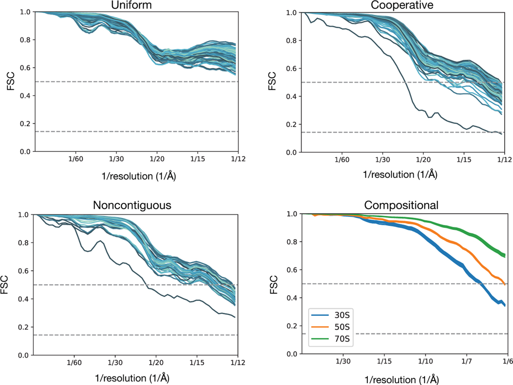
In addition to reconstructing heterogeneous density maps, cryoDRGN produces a latent encoding for each particle that can be compared to the ground truth reaction coordinate (Fig. 3E–H). For the datasets with continuous conformational changes, the latent encoding of each image correlated with position along the reaction coordinate given by the dihedral angle of the underlying model (Spearman r = −0.996, 0.992, and 0.988 for Uniform, Cooperative, and Noncontiguous, respectively) (Fig. 3E). We observed that the qualitative features of the distribution of latent encodings matched the ground truth, with three modes in the latent encoding distribution for the Cooperative dataset (Fig. 3F) and distinct clusters for the Noncontiguous and Compositional datasets (Fig. 3G, H). We note that, in general, the parameterization of a reaction coordinate is non-unique (e.g. when described by the learned latent variable or by dihedral angle, leading to different marginal distributions in Fig. 3E). To quantitatively assess that cryoDRGN has learned the correct distribution of structures, we compute a “per-image” FSC, which compares reconstructed density maps with the ground-truth on images across the reaction coordinate (Methods), and found that the reconstructed structures of all four datasets correlated well with the ground truth distribution (Fig. 3C, Extended Data Fig. 1).

CryoDRGN uncovers residual heterogeneity from “homogeneous” cryo-EM datasets

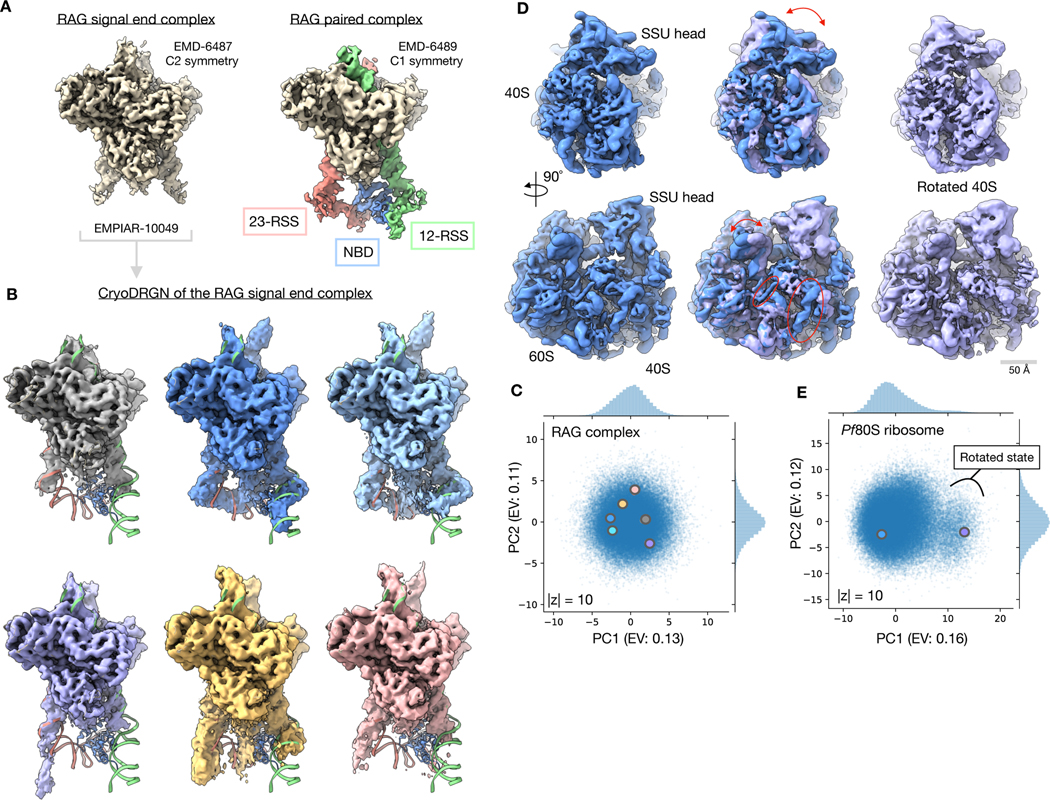
We next evaluated cryoDRGN’s ability to perform heterogeneous reconstruction on real cryo-EM datasets of the RAG complex³¹ and the Pf80S³² ribosome from above. Ru et al. reported RAG complex structures from two distinct datasets – the “signal end complex”, which failed to resolve the distal ends of the 12-RSS and 23-RSS DNA elements or the nonamer binding domain (NBD) of RAG-1; and the “paired complex”, which resolved these elements at sufficient resolution for atomic model building (Fig. 4A). To test whether cryoDRGN could newly uncover heterogeneity of these distal elements in the “signal end complex”, we trained a cryoDRGN 10-D latent variable model on the deposited particle images (EMPIAR-10049)³¹. We found that cryoDRGN revealed significant heterogeneity of the 12-RSS, 23-RSS, and NBD (Fig. 4B). In addition to maps that only resolve the symmetric core (light grey in Fig. 4B), cryoDRGN revealed structures with RSS positioning that aligns with the canonical conformation found in the “paired complex” atomic model³¹ (dark blue), tilting of the RSS strands (light blue), linear 23-RSS DNA (purple), as well as the presence (yellow) and absence (coral) of the NBD. These representative maps were selected out of a large ensemble of generated structures (Methods) from different regions of the latent space (Fig. 4C). A trajectory sampling from the continuous distribution modeled by cryoDRGN is shown in Supplementary Video 1. To validate the presence of these heterogeneous states in the dataset, we performed heterogeneous 3D refinement in cryoSPARC¹⁶ using the cryoDRGN density maps as initial models, which reproduced the heterogeneity of the RSS elements (Extended Data Fig. 2). Subsequent work by Ru et al. suggested that the conformational dynamics and asymmetric positioning of the 12- and 23-RSS by NBD in the pre-cleavage form are fundamental to the structural mechanism underlying the 12–23 rule of V(D)J recombination³³. Our results newly demonstrate that such heterogeneity is also present in the post-cleavage “signal end” RAG complex.

Figure 4. Discovery of residual heterogeneity in “homogeneous” datasets.

A) Published density maps of the 369 kDa RAG1-RAG2 complex. The signal end complex (left) shows the C2 symmetric core and the paired complex (right) resolves additional asymmetric 12- and 23-RSS DNA elements and the RAG-1 nonamer binding domain (NBD) that extend below the core.

B) Representative density maps of the RAG signal end complex (EMPIAR-10049)³¹ reconstructed by cryoDRGN. Density maps resolve variable conformations of the 12- and 23-RSS DNA elements and the nonamer binding domain (NBD) missing from the homogeneous refinement. Docked atomic model (PDB: 3JBW) of the RAG paired complex includes an asymmetric conformation of the RSS and NBD elements outside of the core RAG complex.

C) Latent space representation of particles images from EMPIAR-10049³¹, visualized using PCA with explained variance (EV) noted. Structures from (B) are marked with the corresponding color.

D) Density map of the 4.2 MDa Pf80S ribosome (EMPIAR-10028)³² in an unrotated (blue) and rotated (purple) state reconstructed by cryoDRGN. Arrows indicate rotation of the 40S subunit relative to the 60S subunit (top) and motion of the L1 stalk (bottom). Circles indicate differential occupancy of the C-terminal helix of eL8 and an rRNA helix between the two states.

E) Latent space representation of particle images from EMPIAR-10028³², visualized using PCA with explained variance (EV) noted. Structures from (D) are marked with the corresponding color. A cluster of particles separated along PC1 of (D) that corresponds to the rotated state of the Pf80S ribosome is noted.

Additional density maps from these datasets are shown in Extended Data Figure 2 and Supplemental Videos 1 and 2.

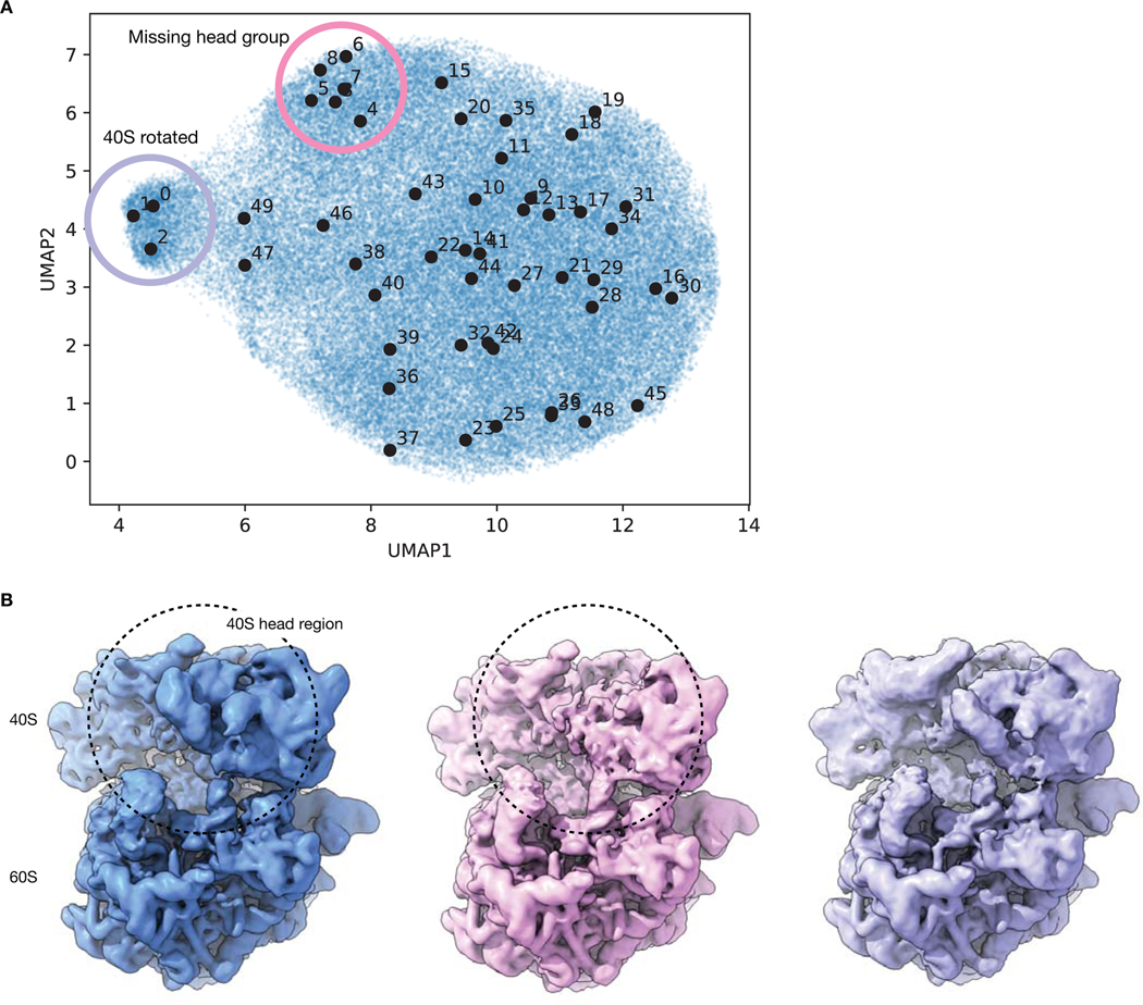
When analyzing a homogeneous reconstruction of the Pf80S ribosome, Wong et al. observed flexibility in the small subunit head region and missing density for peripheral rRNA expansion segment elements³². To explore if this unresolved density resulted from residual heterogeneity, we trained a cryoDRGN 10-D latent variable model on their deposited dataset (EMPIAR-10028)³² and reconstructed an ensemble of density maps that not only contained structures consistent with the homogeneous reconstruction, but also revealed rotation of the 40S small subunit (SSU) (Fig. 4D), heterogeneity within the SSU head (Extended Data Fig. 3), and motion of many peripheral rRNA expansion segments (Supplementary Video 2). By visualizing a representative 40S rotated and unrotated density map, we found that cryoDRGN was able to simultaneously capture the large-scale inter-subunit rotation and coordinated smaller-scale structural rearrangements, including motion of the L1 stalk, disappearance of an rRNA helix, and the disappearance of the inter-subunit bridge formed by the C-terminal helix of eL8, which is consistent with Sun et al.’s characterization of Pf80S dynamics³⁴ (Fig 4D).

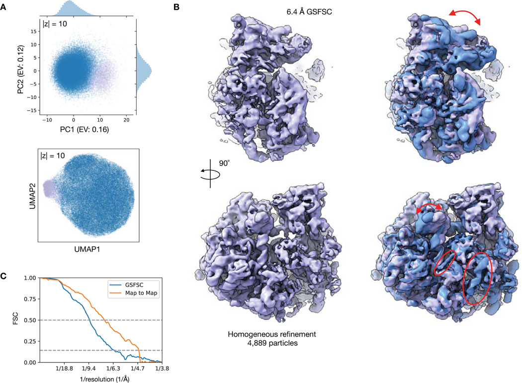
We then visualized the 10-D latent space representation of the Pf80S particles with PCA (Fig. 4E) and with Uniform Manifold Approximate and Projection (UMAP)³⁵ (Extended Data Fig. 4). The 40S rotated density map originated from a region of the particle distribution separated along the first PC of the latent space. To validate the presence of this state, we extracted 4,889 particles constituting the outlying cluster (Methods). Traditional homogeneous reconstruction of these particles in cryoSPARC produced a 6.4 Å reconstruction of the rotated 40S state consistent with the cryoDRGN structure (Extended Data Fig. 4). Additionally, by sampling many density maps from the latent space, we observed that structures with density missing from the SSU head group were located within a subregion of the main cluster of the UMAP visualization (Extended Data Fig. 3). We hypothesize that the 40S rotated state appears as a visually distinct cluster because more mass changes to rotate the entire 40S subunit, as opposed to the missing SSU head group state, which involves changes in a smaller region of the 40S subunit.

CryoDRGN automatically partitions assembly states of the bacterial ribosome

Next, we sought to evaluate cryoDRGN on a highly heterogeneous cryo-EM dataset of the E. coli large ribosomal subunit (LSU) undergoing assembly (EMPIAR-10076)¹². This dataset is known to contain substantial compositional and conformational heterogeneity; In the original analysis, multiple expert-guided rounds of hierarchical 3D classification resulted in 13 discrete structures that were grouped into 4 major assembly states. Here, we aimed to assess if cryoDRGN could automatically reveal these heterogeneous states without user-guided 3D classification.

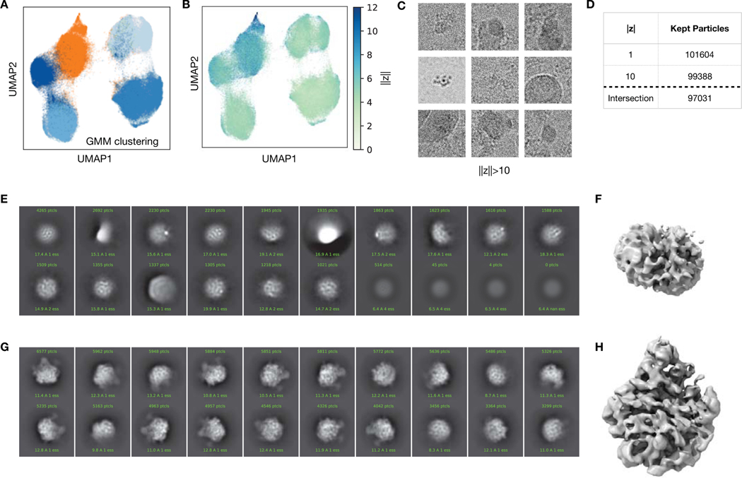
As initial pilot experiments, we first trained 1-D and 10-D latent variable models on downsampled images of the dataset (Methods). The dataset’s latent space representation exhibited distinct peaks in the 1-D case or clusters in the 10-D case when visualized with UMAP³⁵ (Fig. 5A,B) that correspond to the major assembly states when grouped by the published 3D classification labels (Fig. 5C,D). As the particles were obtained by crudely fractionating a lysate in order to capture the full ensemble of cellular assembly intermediates, a substantial fraction of the published particle stack corresponds to 30S or non-ribosomal impurities. These unassigned particles were outliers in the latent representation (Fig 5C, Extended Data Fig. 5), and neither 2D class averages nor a traditional 3D reconstruction of these particles produced structures consistent with assembling LSU ribosomes (Extended Data Fig. 5). As we did not wish to devote representation capacity of the cryoDRGN neural networks in modelling these impurities, we used the latent representation to filter the dataset before further analysis, taking the intersection of the particle stack after filtering based on the 1-D and 10-D latent variable model (Methods).

Figure 5. CryoDRGN heterogeneous reconstruction of the assembly landscape of the bacterial large ribosome subunit.

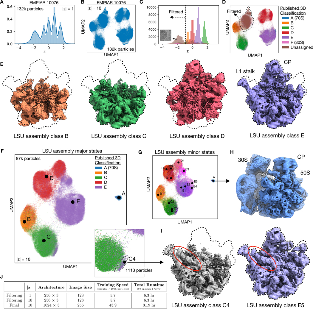
A,B) Latent space representation of particle images of the assembling large ribosomal subunit (LSU) (EMPIAR-10076)¹² as a histogram or UMAP embeddings after training a cryoDRGN 1-D and 10-D latent variable model, respectively.

C,D) Latent space representation of particles colored by major LSU assembly state assigned from 3D classification in Davis et al¹². Impurities in the dataset were assigned and subsequently filtered based on a cutoff of z = −1 in the 1-D case (dotted line), and cluster assignment from a 5-component Gaussian mixture model in the 10-D case. Dotted line in D indicates rough outline of cluster assignment, shown in Extended Data Figure 4.

E) Density maps reconstructed by cryoDRGN of the four major assembly states of the LSU, after training on the filtered dataset. Dotted line indicates outline of the fully mature 50S ribosome.

F,G) Latent space representation of the filtered dataset, colored by major and minor assembly state assigned from 3D classification in Davis et al¹². Points denote cluster centers for the corresponding assembly state. Major assembly state labels correspond to the structures from (E). Inset shows magnified view of the state C cluster, and a population of particles originally mis-classified into state E.

H,I) CryoDRGN reconstruction of additional density maps, showing the 70S ribosome, an impurity during purification, and LSU minor states C4 and E5. Newly identified C4 resembles major state C in maturation, but contains rRNA helix 68, previously present only in mature assembly states E4 and E5.

J) Hyperparameters and runtime of the initial pilot experiments for particle filtering (A-D) and the final cryoDRGN model (E-I) trained on the assembling LSU dataset.

Additional density maps are shown in Extended Data Figure 5 and Supplemental Video 3.

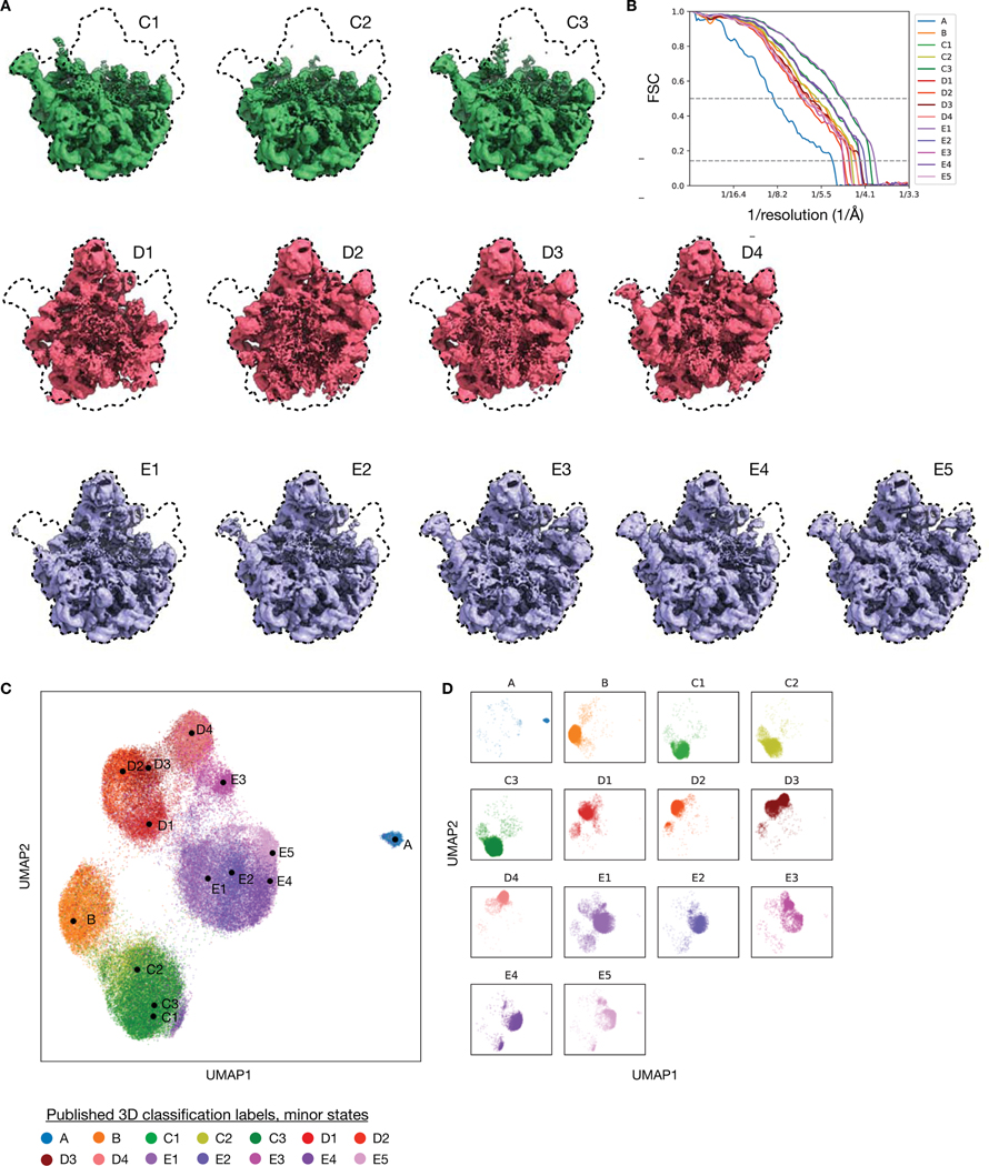
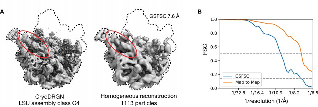
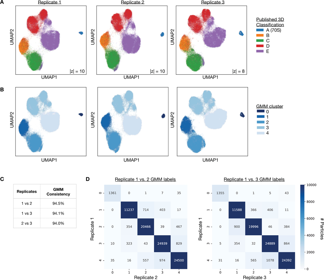
To explore the heterogeneity within the LSU assembly states, we trained a cryoDRGN 10-D latent variable model on the remaining images at higher resolution (Methods). The decoder network reconstructed density maps matching the reported major (Fig. 5E) and minor (Extended Data Fig. 6) assembly states of the LSU. We visualized the encodings of particle images in the 10-D latent space with UMAP and observed clusters corresponding to the major (Fig. 5F) and minor states (Fig. 5G, Extended Data Fig. 6) of LSU assembly after coloring by the published 3D classification. From the latent representation, we also noted a clearly separated cluster of particles assigned to class A, and structures sampled from this region of latent space reconstructed the 70S ribosome, an impurity in the dataset (Fig. 5H). Finally, we identified a small cluster of ~1,100 particles adjacent to the class C cluster whose particles were originally classified into class E (Fig. 5F, inset). The density map reconstructed by the decoder from this region revealed a previously unreported assembly intermediate that we newly define as class C4 (Fig. 5I). Like the other class C structures, class C4 lacked the central protuberance, but possessed clearly resolved density for rRNA helix 68, which was only present in the mature E4 and E5 classes from Davis et al.¹² Traditional homogeneous reconstruction of the particle images constituting this cluster reproduced a similar, albeit lower-resolution structure, which confirmed the existence of this structural state in the original dataset (Extended Data Fig. 7). We found that the cryoDRGN latent representation is highly reproducible across replicates (Extended Data Fig. 8). CryoDRGN experiments and runtimes are summarized in Figure 5J. In addition to illustrating cryoDRGN’s ability to model extremely heterogeneous datasets without user-driver classification, this analysis further demonstrated that cryoDRGN can identify novel and rare (~1% of all particles) structural classes that would likely be overlooked by traditional hierarchical classification.

CryoDRGN reveals dynamic continuous motions in the pre-catalytic spliceosome

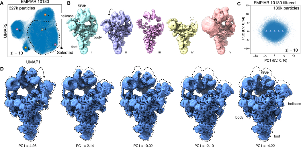
Finally, to assess cryoDRGN’s ability to model large continuous conformational changes, we reanalyzed a dataset of the pre-catalytic spliceosome (EMPIAR-10180)³⁶. Using extensive, expert-guided focused classifications, Plaschka et al. reconstructed a composite map for this complex and suggested that the complex sampled a continuum of conformations with large motions of the SF3b subcomplex³⁶. In our analysis, we first trained a 10-D latent variable model on the downsampled images using image poses derived from a consensus reconstruction (Methods). Multiple clusters were observed in the latent space encodings of the dataset’s particle images (Fig. 6A). In sampling structures from the latent space, the generated density maps revealed expected spliceosome conformations from the largest cluster, poorly resolved structures likely due to imaging artifacts from the leftmost cluster, structures lacking density for the SF3b subcomplex from a third cluster, and extra density of the U2 core, which is thought to be highly dynamic¹³, from the uppermost cluster (Fig. 6B). To focus our analysis on bone-fide pre-catalytic spliceosome particles, we leveraged the latent space representation to eliminate any particles that mapped to the undesired clusters from two replicate runs (Methods).

Figure 6. CryoDRGN heterogeneous reconstruction of the pre-catalytic spliceosome.

A) UMAP visualization of the latent space representation of particle images of pre-catalytic spliceosome (EMPIAR-10180)³⁶ after training a 10-D latent variable model with cryoDRGN.

B) Representative structures generated at points shown in (A) that depict the expected structures of the pre-catalytic spliceosome (i,ii), structures likely corrupted by imaging artifacts (iii), the complex lacking the SF3b subcomplex (iv), and with the U2 core (v). Density maps are shown at identical isosurface levels except for (v) which required a lower value to highlight the U2 core.

C) PCA projection of latent space encodings after training a 10-D latent variable model on the dataset filtered for the selected region in (A).

D) Structures generated by traversing along PC1 of the latent space representation at points shown in (C).

Additional density maps are shown in Extended Data Figure 7 and Supplemental Video 4.

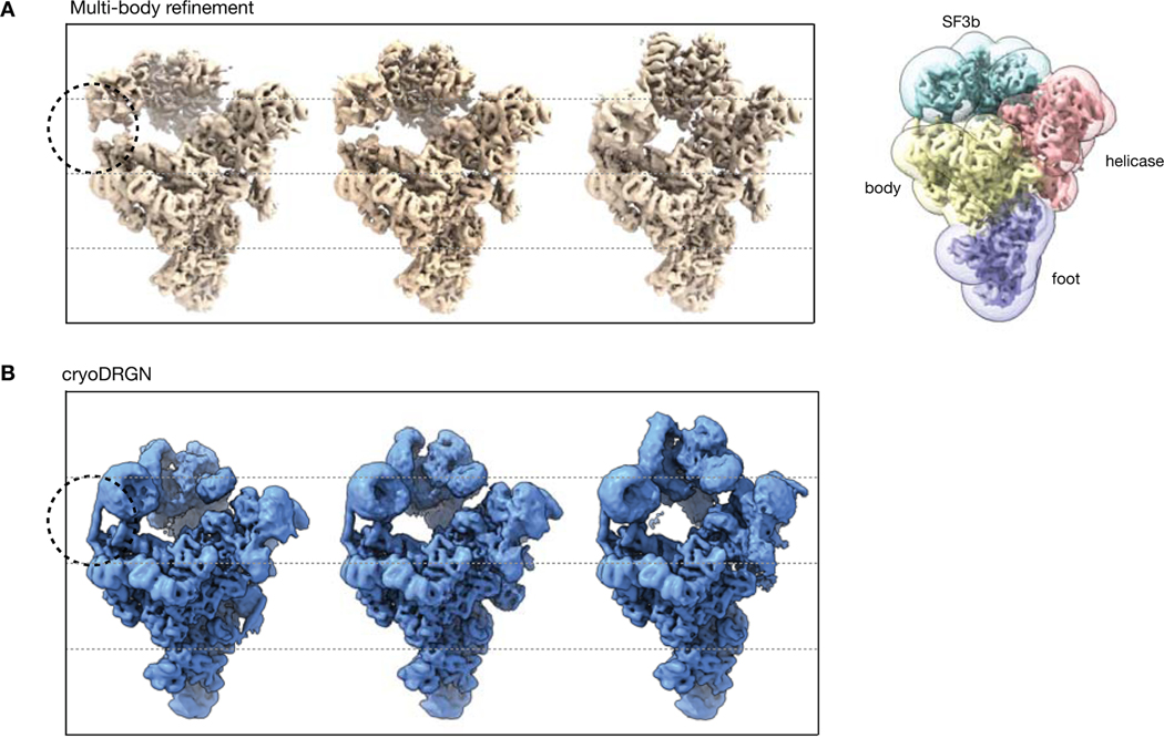
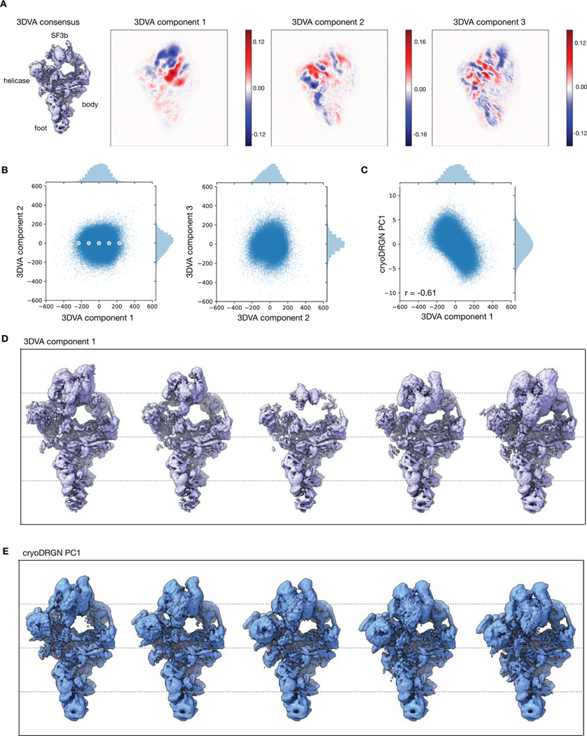
With the filtered particle stack, we trained a 10-D model on higher resolution images and visualized the dataset’s latent encodings in 2-D using PCA (Fig. 6C). The visualized data manifold was unfeatured, consistent with a molecule undergoing non-cooperative conformational changes. By generating structures along the first principal component of the latent space encodings, we reconstructed a trajectory of the SF3b and helicase subcomplexes in motion, smoothly transitioning from an elongated state to one compressed against the body of the spliceosome (Fig. 6D). This large scale-motion is consistent with motions derived from the first principal component of rigid body orientations from multi-body analysis (Extended Data Fig. 9) and in the first principal component of 3DVA’s linear subspace model (Extended Data Fig 10). A similar traversal along the second PC produced a continuous trajectory of the SF3b and helicase subcomplexes moving in opposition (Supplementary Fig. 1, Supplementary Video 4). The anticorrelated motion of the SF3b and helicase subcomplexes in PC2, together with their correlated motion in PC1, suggests that the two domains move independently in the imaged ensemble. Finally, although trajectories along latent space PCs provide a summary of the extent of variability in the structure, cryoDRGN can also generate structures at arbitrary points from the latent space. By traversing along the nearest neighbor graph of the latent encodings and generating structures at the visited nodes, cryoDRGN generated a plausible trajectory of the conformations adopted by the pre-catalytic spliceosome (Supplementary Video 4), highlighting the potential of single particle cryo-EM to uncover the conformational dynamics of molecular machines.

Discussion

This work introduces cryoDRGN, a method using neural networks to reconstruct 3D density maps from heterogeneous single particle cryo-EM datasets. The power of this approach lies in its ability to represent heterogeneous structures without simplifying assumptions on the type of heterogeneity. In principle, cryoDRGN is able to represent any distribution of structures that can be approximated by a deep neural network, a broad class of function approximators for continuous, nonlinear functions²⁸. This flexibility contrasts with existing methods that impose limiting assumptions on the types of structural heterogeneity present in the sample. For example, 3D classification assumes a mixture of discrete structural classes; multibody refinement assumes conformational changes are composed of user-defined rigid-body motions; and 3DVA assumes that heterogeneity is generated from linear combinations of density maps. Although these approaches have proven useful, their model for heterogeneity is often mismatched with the true structural heterogeneity in many systems, and thus can introduce bias into reconstructions. In contrast, we empirically show that the cryoDRGN architecture can model both discrete compositional heterogeneity and continuous conformational changes without the aforementioned structural assumptions. For example, we discovered heterogeneous states of the RAG complex and Pf80S ribosome that were originally averaged out of the homogeneous reconstruction. When analyzing the assembling E. Coli LSU dataset, cryoDRGN learned an ensemble of LSU assembly states without a priori specification of the number of states or initial models as is required for 3D classification. Finally, when analyzing the pre-catalytic spliceosome, we found that the continuous conformational changes reconstructed by cryoDRGN lacked the rigid-body boundary artifacts from multibody refinement’s mask-based approach¹⁹ (Extended Data Fig. 9) or linear interpolation artifacts from 3DVA’s linear subspace model²³ (Extended Data Fig. 10).

Interpretation of the latent space

A key feature of cryoDRGN is its ability to provide a low-dimensional representation of the dataset’s heterogeneity given by each particle’s latent encoding. Subject to optimization, cryoDRGN organizes the latent space such that structurally related particles are in close proximity. In simulated and real datasets, we find that continuous motions are embedded along a continuum in latent space (Fig. 3E–G, 6C) and that compositionally distinct states manifest as clusters (Fig. 3H, 5F). These empirical results demonstrate that visualization of the distribution of latent encodings can be informative in exploring the structural heterogeneity within the imaged ensemble, and even suggest a possible interpretation of the latent space as a pseudo-conformational landscape. However, we note that cryoDRGN’s objective function aims only to reproduce the distribution of structures and does not guarantee that the latent space layout (or its 2D visualization) will produce interpretable features of the underlying energy landscape. Furthermore, structures reconstructed from unoccupied regions of the latent space will not in general correspond to true physical structures, as cryoDRGN optimizes the likelihood of the observed data and these structures are not observed.

Finally, in real datasets, there may exist images that do not originate from the standard single particle image formation model, for example, false positives encountered during particle picking. We demonstrated the utility of the latent space representation in identifying such impurities, ice artifacts, and other out-of-distribution particle images that may be filtered out in subsequent analyses (Fig. 5A–D, 6A).

We emphasize that different datasets have diverse sources of heterogeneity, and thus the interpretation of the cryoDRGN latent space is highly dataset-dependent. We provide interactive analysis tools in the cryoDRGN software for exploring the learned latent space.

Visualizing structural trajectories

In addition to encoding particles in an unsupervised manner, cryoDRGN can reconstruct 3D density maps from user-defined positions in latent space. Because cryoDRGN learns a generative model for structure, an unlimited number of structures can be generated and analyzed, thus enabling visualization of structural trajectories. By leveraging the latent encodings of the particle images, users can directly traverse the data manifold and only sample structures from regions of latent space with significant particle occupancy. Indeed, we applied a well-established graph-traversal algorithm³⁷ to visualize data-supported motions in the RAG complex, the Pf80S ribosome, bL17-independent assembly of the bacterial ribosome, and the pre-catalytic spliceosome (Supplemental Videos 1,2,3,4). We note that while this approach is useful in visualizing potential structural changes linking one state to another, they do not necessarily reveal the kinetically preferred path.

Practical considerations in choosing training hyperparameters

Although this method emphasizes an unsupervised approach to analyzing structural heterogeneity, cryoDRGN does require that the user define the dimensionality of the latent space and the architecture of both the encoder and decoder networks. We find that in practice, training a smaller architecture on downsampled images is effective at distinguishing bona-fide particles from contaminants and imaging artifacts (Fig. 5A–D, Fig. 6A), and we recommend users initially employ such pilot experiments to filter their dataset. Additionally, we find that in our tested datasets, a 10-D latent space provides sufficient representation capacity to effectively model structural heterogeneity, and that this 10-D space can be readily visualized with PCA or UMAP. Notably, we recommend the use of such a 10-D latent space instead of lower dimensional space as we have found that 10-D spaces result in much more rapid overall training, which is consistent with similar observations of related overparameterized neural network architectures³⁸. Finally, users must specify the number of nodes and layers in the neural networks, hyperparameters that limit the complexity of the learned function. Here, we find an inverse relationship between neural network size and the achievable resolution of a given structure (Fig. 2B). Training larger networks on larger images is significantly slower (Fig. 2E), and we recommend that users perform an initial assessment using down-sampled images and relatively small networks before proceeding to high-resolution reconstructions. We note that use of excessively complex models (i.e. large architectures or latent variable dimensions) can lead to overfitting, which may be alleviated by standard neural network regularization techniques such as early stopping or using a simpler model³⁸. We provide recommended training settings in the cryoDRGN software.

Discovering new states using cryoDRGN

CryoDRGN can be used to identify novel clusters of structurally-related particles, which can then be visualized by generating density maps from that region of latent space. Indeed, in analyzing the LSU assembly dataset, we noted a completely new structural state, C4, that was completely missed in traditional hierarchical classification. C4 provides structural evidence that a functionally critical intersubunit helix (h68) can dock in a native conformation in the absence of the central protuberance (Fig. 5I). Notably, we could validate the existence of this state by performing traditional homogeneous refinement using ~1,000 particles from this cluster in the cryoDRGN latent space (Extended Data Fig. 7). Although we were able to readily identify this state from a distinct cluster present in the UMAP visualization (Fig. 5G), in general, the definition of distinct “states” may not be as readily apparent (e.g. the “missing SSU head” state in Extended Data Fig. 3), and we view the unsupervised identification of states from the cryoDRGN structural ensemble as an exciting area to pursue.

In future work, we envision using cryoDRGN to reveal the number of discrete classes, their constituent particles, and to produce initial 3D models that could be used as inputs for a traditional 3D reconstruction. Given the mature state of such tools^39,40, this data-driven classification approach followed by traditional homogeneous reconstruction, particle polishing, and higher order image aberration correction, has the potential to produce high-resolution structures of the full spectrum of discrete structural states.

De novo pose estimation

As implemented, cryoDRGN uses pose estimates resulting from a traditional consensus 3D reconstruction. In analyzing four publicly available datasets, we found that such consensus pose estimates were sufficiently accurate to generate meaningful latent space encodings and to produce interpretable density maps of distinct structures. It is clear, however, that this approach will fail if the degree of structural heterogeneity in the dataset results in inaccurate pose estimates. For example, a mixture of structurally unrelated complexes will align poorly to a consensus structure, and thus produce poor pose estimates. Notably, our framework is differentiable with respect to pose variables, which, in principle, should allow for on-the-fly pose-refinement or de novo pose estimation. Future work will explore the efficacy of incorporating such features to enable fully unsupervised reconstruction of heterogeneous distributions of protein structure from cryo-EM images.

Online Methods

The cryoDRGN method

Coordinate-based networks to represent 3D structure

The cryoDRGN method performs heterogeneous cryo-EM reconstruction by learning a neural network representation of 3D structure. In particular, we use a positionally-encoded multilayer perceptron (MLP) to approximate the function V: ℝ³⁺ⁿ → ℝ, which models structures as generated from an n-dimensional continuous latent space. We refer to this architecture as a coordinate-based neural network^41,42 as we explicitly model the volume as a function of Cartesian coordinates.

Without loss of generality, we model volumes on the domain [−0.5,0.5]³. Instead of directly supplying the 3D Cartesian coordinates, k, to the deep coordinate network, coordinates are featurized with a fixed positional encoding function⁴³ consisting of sinusoids whose wavelengths follow a geometric progression from 1 up to the Nyquist limit:

$$p{e}^{(2i)}\left(k_j\right)=\sin \left(k_{j}D\pi {\left(\frac{2}{D}\right)}^{\frac{i}{\left(\frac{D}{2}-1\right)}}\right),i=0,\dots ,\frac{D}{2}-1;k_j\in \mathit{k}$$

$$p{e}^{(2i+1)}\left(k_j\right)=\cos \left(k_{j}D\pi {\left(\frac{2}{D}\right)}^{\frac{i}{\left(\frac{D}{2}-1\right)}}\right),i=0,\dots ,\frac{D}{2}-1;k_j\in \mathit{k}$$

where D is set to the image size¹ used in training. Empirically, we found that excluding the highest frequencies of the positional encoding led to better performance when training on noisy data, and we provide an option to modify the positional encoding function by increasing all wavelengths by a factor of 2π.

Training system

This neural representation of 3D structure is learned via an image-encoder/volume-decoder architecture based on the variational autoencoder (VAE)^30,44. We follow the standard image formation model in single particle cryo-EM where observed images are generated from projections of a volume at a random unknown orientation, R ∈ SO(3). We use an additive Gaussian white noise model. Volume heterogeneity is generated from a continuous latent space, modeled by the latent variable z, where the dimensionality of z is a hyperparameter of the model.

Given an image X, the variational encoder, q_ξ(z|X), produces a mean and variance, μ_z|X and Σ_z|X, statistics that parameterize a Gaussian distribution with diagonal covariance, as the variational approximation to the true posterior p(z|X). The prior on the latent variable is a standard normal distribution $\mathcal{N}$(0, I). The positionally-encoded MLP is used as the probabilistic decoder, p_θ(V| k, z), and models structures in frequency space. Given Cartesian coordinate k ∈ ℝ³ and latent variable z, the probabilistic decoder predicts a Gaussian distribution over V(k, z). The encoder and decoder are parameterized with fully connected neural networks with parameters ξ and θ, respectively.

Since 2D projection images can be related to volumes as 2D central slices in Fourier space²⁹, oriented 3D coordinates for a given image can be obtained by rotating a D × D lattice spanning [−0.5,0.5]² originally on the x-y plane by R, the orientation of the volume during imaging. Then, given a sample out of q_ξ(z|X) and the oriented coordinates, an image can be reconstructed pixel-by-pixel through the decoder. The reconstructed image is then translated by the image’s in-plane shift and multiplied by the CTF before it is compared to the input image. The negative log likelihood of a given image under our model is computed as the mean square error between the reconstructed image and the input image. Following the standard VAE framework, the optimization objective is a variational lower bound of the model evidence:

$$\mathcal{L}(X;\xi ,\theta )=E_{q_{\xi }(\mathit{z}\mid X)}[\log p(X\mid \mathit{z})]-\beta KL\left(q_{\xi }(\mathit{z}\mid X)\parallel p(\mathit{z})\right)$$

where the first term is the reconstruction error estimated with one Monte Carlo sample, the second term is a regularization term on the latent representation, and β is an additional hyperparameter, which we set by default to 1/|z|. By training on many 2D slices with sufficiently diverse orientations, the 3D volume can be learned through feedback from the 2D views. For further details, we refer the reader to a preliminary version of the method described in the proceedings of the International Conference for Learning Representations⁴¹. The results presented here employ the training regime described in Zhong et al. using previously determined poses from a consensus reconstruction⁴¹.

Datasets

Simulated compositionally heterogeneous dataset generation

To generate the compositionally heterogeneous dataset, the 30S, 50S and 70S subunits of the E. coli ribosome were extracted from PDB 4YBB in PyMOL⁴⁵. A density map of each subunit was generated from the atomic model using the molmap⁴⁶ command in Chimera⁴⁷ at a grid spacing of 1.5 Å/pix and a resolution of 4.5 Å. The resulting volume was padded to a box size of D=256, where D is the width in pixels along one dimension. Simulated particle images were generated with a custom Python script available in the cryoDRGN software by rotating the density map with a random rotation sampled uniformly from SO(3), projecting along the z-axis, and shifting the image with an in-plane translation sampled uniformly from [−20,20]² pixels. Images were then downsampled to D=128 by Fourier clipping using a custom Python script, corresponding to a Nyquist limit of 6 Å. Projection images were multiplied with the CTF in Fourier space, where the CTF was computed from defocus values randomly sampled from those given in EMPIAR-10028³², no astigmatism, an accelerating voltage of 300 kV, a spherical aberration of 2 mm, and an amplitude contrast ratio of 0.1. An envelope function with a B-factor of 100 Ų was applied. Noise was added with a signal to noise ratio (SNR) of 0.1 where the noise-free signal images were defined as the entire D × D image. After performing this procedure for each subunit, 10k, 15k, and 25k simulated particles of the 30S, 50S, and 70S ribosome, respectively, were combined.

Simulated conformationally heterogeneous dataset generation

To simulate continuous conformational heterogeneity, 50 density maps were generated along a one-dimensional reaction coordinate defined by rotating a dihedral angle in an atomic model of a hypothetical protein complex. Each model was generated at 0.03 radian increments of the bond rotation, leading to a total range of 1.5 radians. Density maps were generated using the molmap⁴⁶ command in Chimera⁴⁷ at a grid spacing of 6 Å/pix and resolution of 12 Å, and padded to a box size of D=128. For the Uniform dataset, 1000 projection images were generated for each density map at random orientations and in-plane translations sampled from [−10,10]² pixels. For the nonuniform datasets, particles were generated along the reaction according to a 3-component Gaussian mixture model with means at the 10^th, 25^th, and 40^th density map and standard deviation of 0.09 and 0.03 radians for the Cooperative and Noncontiguous datasets, respectively. Sampled reaction coordinate values were binned to convert into a particle distribution among the 50 generated density maps, and clipped at values of the reaction coordinate beyond the 50 maps. A total of 50k particles were generated for each dataset. CTF and noise at an SNR=0.1 were added to all datasets using the same procedure described above with CTF defocus values randomly sampled from EMPIAR-10028³².

Real cryo-EM datasets

Picked particles and the star file containing CTF parameters were downloaded from the Electron Microscopy Public Image Archive (EMPIAR)⁴⁸ for datasets EMPIAR-10049, EMPIAR-10028, EMPIAR-10076, and EMPIAR-10180. Particle images were downsized to the image size used in training by clipping in Fourier space with a custom Python script available in the cryoDRGN software.

Consensus reconstructions

Homogeneous 3D reconstruction of the Pf80S ribosome (EMPIAR-10028) was performed in cryoSPARC v2.4¹⁶ using the ab-initio reconstruction job followed by the homogeneous refinement job with default parameters. The final reconstruction reported a GSFSC_0.143⁴⁹ resolution of 3.1 Å with a tight mask and 4.1 Å unmasked.

Homogeneous 3D reconstruction of the bL17-depleted ribosome assembly intermediates (EMPIAR-10076) was performed as above, leading to a final structure with a GSFSC_0.143 resolution of 3.2 Å with a tight mask and 4.8 Å unmasked.

Homogeneous 3D reconstruction of the RAG complex (EMPIAR-10049) was performed as a “Homogeneous Refinement (NEW!)” job in cryoSPARC v2.15 with all default settings, including C1 symmetry. The asymmetric PC map of the RAG complex was used as an initial model (EMDB 6489), low pass filtered by 30 Å. The final structure had GSFSC_0.143 resolution of 3.6 Å with a tight mask and 4.6 Å unmasked.

Poses from a consensus reconstruction of the pre-catalytic spliceosome were obtained from the star file deposited in EMPIAR-10180.

CryoDRGN homogeneous reconstruction

CryoDRGN decoder networks with no input latent variable were trained for 50 epochs on full-resolution images of the RAG complex (D=192, 1.23 Å/pix) and the Pf80S ribosome (D=360, 1.34 Å/pix). The tested architectures were MLPs with ReLU activations, where the network size was either 3 hidden layers of width 128 (denoted 128 × 3), 256 × 3, 512 × 3, 1024 × 3, or 1024 × 10. Image poses were set to poses obtained from a consensus reconstruction in cryoSPARC, described above¹⁶. Networks were trained on minibatches of 8 images using the Adam optimizer with a learning rate of 0.0001. Once training completed, the decoder network was evaluated on the 3D coordinates of a D × D × D voxel array spanning [−0.5,0.5]³, where D is the image size in pixels along one dimension. For visualization in Figure 2, the RAG complex density maps were sharpened by −54 Ų and −127.4 Ų for the cryoDRGN and cryoSPARC map, respectively, based on Guinier analysis⁴⁹ performed in a custom Python script; both the cryoSPARC and cryoDRGN density maps of the Pf80S ribosome were sharpened using the published B-factor of −80.1 Ų.

Map-to-map FSC

Fourier shell correlation curves were computed between the cryoSPARC density maps and cryoDRGN density maps using a custom Python script available in the cryoDRGN software. Real space masks were defined by first thresholding the cryoDRGN volume at half of the 99.99th percentile density value. The mask was then dilated by 25 Å from the original boundary, and a soft cosine edge was used to taper the mask to 0 at 15 Å from the dilated boundary.

CryoDRGN heterogeneous reconstruction

Model training

A summary of the datasets, hyperparameters, and runtimes for all cryoDRGN heterogeneous reconstruction experiments is given in Supplementary Table 1. CryoDRGN encoder-decoder networks were trained from their randomly initialized values for each single particle cryo-EM dataset. Image poses used for training were either the ground truth poses for simulated datasets or poses obtained from a consensus reconstruction as described above. All networks were trained on minibatches of 8 images using the Adam optimizer with a learning rate of 0.0001. After training, the dataset images were evaluated through the encoder to obtain the latent encoding for each image. We define the latent encoding as the maximum a posteriori value of q_ξ(z|X) predicted by the encoder.

Latent space visualization

For latent spaces with dimension greater than 2, the distribution of latent encodings were visualized with standard dimensionality reduction techniques such as PCA and UMAP³⁵. PCA projections of latent space particle distributions were computed using the implementation provided by scikit-learn⁵⁰. Two-dimensional UMAP³⁵ embeddings were computed using version 0.4.1 of the Python implementation (https://github.com/lmcinnes/umap) with the default settings of k=15 for the k-nearest neighbors graph and a minimum distance parameter of 0.1. Automated tools to analyze and visualize the latent space given the outputs of model training are provided in the cryoDRGN software.

Density map generation

Density maps were generated for a given value of the latent variable z by evaluating the trained decoder on z and the 3D coordinates of a D × D × D voxel array spanning [−0.5,0.5]³. For higher dimensional latent spaces (|z| > 1), to generate representative samples from different regions of the latent space, we perform k-means clustering of the dataset’s latent encodings to partition the latent space into k regions. A representative density map for each region is generated at the “on-data” cluster center; We define the latent encoding closest in Euclidean distance to the k-means cluster center as the “on-data” cluster center. Automated tools to generate k representative density maps following this procedure are provided in the cryoDRGN software.

Heterogeneous reconstruction of simulated datasets

For each simulated heterogeneous dataset, a 1-D latent variable model was trained for 100 epochs. The encoder architecture was 256 × 3 and the decoder architecture was 512 × 5. The image poses used for training were the ground truth image poses. After training on the Uniform simulated dataset, structures shown in Figure 3C were generated at the 5th, 23rd, 41st, 59th, 77th, and 95^th percentile values of the latent encodings, and sharpened by a B-factor of −100 Ų. After training on the Compositional simulated dataset, structures shown in Figure 3D were generated at the k-means cluster centers after performing k-means clustering with k=3 on the latent encodings and sharpened by a B-factor of −100 Ų. Spearman correlation was computed using the implementation provided in the scipy version 1.5.2 Python package (https://www.scipy.org).

Per-image FSC

For simulated datasets where the ground-truth distribution of structures is known, “per-image” FSC curves can be computed between cryoDRGN-reconstructed density maps and the ground-truth density maps to quantitatively evaluate the reconstructed ensemble. To compute a per-image FSC, an FSC curve is computed between the density map generated by the cryoDRGN decoder at the value of the latent variable predicted for a given particle image and the ground-truth density map used to generate the image. 100 images randomly sampled according to the ground truth distribution of structures were used in the assessment of each of the simulated datasets. No real-space mask was used in computing the FSC.

Heterogeneous reconstruction of the RAG complex (EMPIAR-10049)

A 10-D latent variable model was trained on full-resolution particle images from EMPIAR-10049 (D=192, 1.23 Å/pix) and their consensus reconstruction poses for 25 epochs. The encoder and decoder architectures were 1024 × 3.

Density map generation:

After training, k-means clustering with k=100 was performed on the predicted latent encodings for the dataset, and volumes were generated at the “on-data” cluster centers using the decoder network. Six structurally diverse representative structures were manually selected for visualization in Figure 4A.

Traditional heterogeneous refinement:

To validate the heterogeneous RSS and NBD conformations observed in cryoDRGN, we use the 6 selected density maps, low pass filtered by 20 Å, as initial models to a heterogeneous refinement job in cryoSPARC v2.15.

Heterogeneous reconstruction of the 80S ribosome (EMPIAR-10028)

Pilot experiments:

A 10-D latent variable model was trained on downsampled images (D=128, 3.78 Å/pix) from EMPIAR-10028 and their consensus reconstruction poses for 50 epochs. The encoder and decoder architectures were 256 × 3.

Particle filtering:

After training, k-means clustering with k=20 was performed on the predicted latent encodings for the dataset. One cluster contained 860 particles that were outliers when viewing the projected encodings along the first and second principal component. This observation was reproducible, and the particles belonging to the outlier cluster from either of two replicates (960 particles in total) were removed from the dataset.

High-resolution training:

After particle filtering, a 10-D latent variable model was trained on a random 90% the remaining 104,280 images (D=256, 1.88 Å/pix) for 25 epochs. The encoder and decoder architectures were 1024 × 3.

Density map generation:

After training, k-means clustering with k=50 was performed on the predicted latent encodings for the dataset, and volumes were generated at the “on-data” cluster centers using the decoder network. A representative structure of the rotated state and the unrotated state were manually selected for visualization in Figure 4B. A representative structure of the missing head group state was manually selected for visualization in Extended Data Figure 3. The numbered k-means cluster centers shown in Extended Data Figure 3A, originally arbitrarily ordered, were reordered based on hierarchical clustering of the latent encodings with Euclidean distance metric and average linkage.

Validation with traditional reconstruction:

To validate the 40S rotated state, we selected 4,889 particles as the cluster from k-means clustering with k=20 that was separated along PC1 (Extended Data Fig. 4). These particles were then input to a homogeneous refinement job in cryoSPARC v2.15. The cryoDRGN density map, low pass filtered by 30 Å, was used as the initial model.

Heterogeneous reconstruction of the assembling 50S ribosome (EMPIAR-10076)

Pilot experiments:

A 1-D and a 10-D latent variable model were trained on downsampled images (D=128, 3.3 Å/pix) from EMPIAR-10076 with poses from a consensus reconstruction for 50 epochs. The encoder and decoder architectures were 256 × 3.

Particle filtering:

From the 1-D experiment, particles with z ≤ −1 were removed from subsequent analysis. From the 10-D experiment, a 5-component, full-covariance Gaussian mixture model (GMM) was fit to the latent encodings using scikit-learn⁵⁰, and particles from the outlier cluster were removed. The outlier cluster was identified by visualizing the magnitude of the latent encodings (Extended Data Fig. 4). The intersection of both filtered particles stacks was used for subsequent analysis. 2D classification of the kept and removed particles was performed in cryoSPARC v2.4¹⁶ using all default options except for the number of 2D classes, which was set to 20. Ab-initio reconstruction of the kept and removed particles was performed in cryoSPARC v2.4¹⁶ using all default options.

High-resolution training:

A 10-D latent variable model was trained on a random 90% of the remaining 97,031 images (D=256, 1.7 Å/pix) for 50 epochs. The encoder and decoder architectures were 1024 × 3. Two additional replicates were run, one with the exact settings from a different random initialization and a second with latent variable dimension |z| = 8.

Density map generation:

After training, the dataset’s latent encodings were viewed in 2D with UMAP³⁵. Density maps corresponding to the major and minor assembly states were generated at the “on-data” mean latent encoding for each class, i.e. ${\widehat{\mathit{z}}}_M=\frac{1}{|M|}{\displaystyle {\sum }_{i\in M}{\mathit{z}}_i}$, where M is the set of particles assigned to a given class in the published 3D classification.

Map-to-map FSC:

The map-to-map FSC was computed between the cryoDRGN and published density map for each minor class. Density maps were aligned in Chimera and a loose real-space mask (obtained as described above) was applied before computing an FSC curve.

Reproducibility analysis:

For each replicate, a 5-component, full-covariance GMM was fit to the UMAP embeddings using scikit-learn⁵⁰. UMAP axes were negated to facilitate visual comparison. Label assignments were permuted to ensure consistent assignments between replicates. Clustering consistency was computed as the percentage of particles with identical GMM labels.

New assembly state C4:

Particles corresponding to the new assembly state were manually selected from the UMAP embeddings with an interactive lasso tool in a custom visualization script available in the cryoDRGN software, whose outline is shown in the Figure 5F inset. The mean latent encoding of the resulting 1,113 selected particles was used to generate the structure representative for this new assembly state.

Validation of C4 with traditional refinement:

The particles associated with class C4 were then input to a homogeneous refinement job in cryoSPARC v2.15. The cryoDRGN density map, low pass filtered to 30 Å, was used as the initial model.

Heterogeneous reconstruction of the pre-catalytic spliceosome (EMPIAR-10180)

Pilot experiments:

A 10-D latent variable model was trained on downsampled images (D=128, 4.25 Å/pix) from EMPIAR-10180 for 50 epochs. The encoder and decoder architectures were 256×3. Poses were obtained from the consensus reconstruction values given in the consensus_data.star deposited to EMPIAR-10180.

Particle filtering:

The UMAP embeddings showed multiple clusters where the largest cluster corresponded to fully formed pre-catalytic spliceosomes. Particles corresponding to other clusters were removed from subsequent analyses by first performing k-means clustering with k=20 on the latent encodings, and removing k-means clusters whose structure did not resemble the fully formed pre-catalytic spliceosome (11 out of 20 k-means clusters in one replicate, and 10 out of 20 in a second replicate).

High-resolution training:

A 10-D latent variable model was trained on a random 90% of the remaining 155,247 images (D=256, 2.1 Å/pix) for 50 epochs. The encoder and decoder architectures were 1024 × 3.

Density map generation:

After training, the dataset’s latent encoding was viewed in 2-D with UMAP and PCA. Density maps in Figure 6D were generated at the latent encoding values along the PC1 axis at five equally spaced points between the 5^th and 95^th percentile of PC1 values. Density maps in Supplementary Figure 1 were generated at the latent encoding values along the PC2 axis at five equally spaced points between the 5^th and 95^th percentile of PC2 values. Density map generation along PC axes is implemented in a custom script in the cryoDRGN software.

Latent space graph traversal for generating trajectories

Trajectories were generated by first creating a nearest-neighbors graph from the latent encodings of the images, where a neighbor was defined if the Euclidean distance was below a threshold computed from the statistics of all pairwise distances. We choose a value for each dataset such that the average number of neighbors across all nodes is 5. Edges were then pruned such that a given node does not have more than 10 neighbors. Then, Djikstra’s algorithm³⁷ was used to find the shortest path along the graph connecting a series of anchor points, and density maps were generated at the z value of the visited nodes. Anchor points were either defined manually or set to be the “on-data” cluster centers after performing k-means clustering of the latent encodings.

For the graph traversal of the RAG complex in Supplemental Video 1, we use the latent encodings of the 6 density maps shown in Figure 4A as the anchor points. For the graph traversal of the Pf80S ribosome in Supplemental Video 2, we use 10 randomly chosen latent encodings as the anchor points out of the k-means cluster centers with k=20 that are shown prior to the graph traversal. For the graph traversal of the assembling ribosome in Supplemental Video 3, we use the latent encodings of the minor assembly states following the three assembly pathways given in Figure 7 of Davis et al¹². For the graph traversal of the pre-catalytic spliceosome in Supplemental Video 4, we use the latent encodings of the k-means cluster centers with k=20 as the anchor points. All density map figures and trajectories were prepared with ChimeraX⁵¹ and are viewed at identical isosurface levels for a given model unless otherwise specified. CryoDRGN’s graph traversal algorithm is provided in the cryoDRGN software.

3DVA

3D Variability Analysis²³ was performed in cryoSPARC v2.15 on the 139,722 particles and their consensus poses comprising the filtered EMPIAR-10180 dataset used in cryoDRGN analysis. Three variability modes were solved with all default options and the low-pass filter resolution set to 7 Å. 3DVA per-particle latent encodings were extracted from the cryoSPARC metadata file. Spearman correlation was computed using the implementation provided in the scipy version 1.5.2 Python package (https://www.scipy.org). To visualize the component 1 trajectory in Extended Data Figure 10, the consensus density map was combined with the component 1 eigen-volume at 5 equally spaced points between the 1^st and 99^th percentile value of the 3DVA component 1 latent encoding distribution.

Data Availability Statement

Trained cryoDRGN models and generated volumes are deposited to Zenodo at doi:10.5281/zenodo.4355284. Inputs files for training (excluding particle stacks) are deposited to Zenodo at doi:10.5281/zenodo.4412072 and are also available at www.github.com/zhonge/cryodrgn_empiar. We used the following publicly available datasets:

• EMPIAR-10049: Cryo-EM structures of a synaptic RAG1-RAG2 complex

• EMPIAR-10028: Cryo-EM structure of a Plasmodium falciparum 80S ribosome bound to the anti-protozoan drug emetine

• EMPIAR-10076: Modular assembly of the large bacterial ribosome

• EMPIAR-10180: Structure of a pre-catalytic spliceosome

The simulated datasets of conformational and compositional heterogeneous are deposited to Zenodo at doi:10.5281/zenodo.4355284.

Code Availability Statement

CryoDRGN software and analysis scripts are implemented in custom software deposited to Zenodo at doi:10.5281/zenodo.4412058 and are also available at www.github.com/zhonge/cryodrgn.

Extended Data

Extended Data Figure 1. Per-image FSC curves between ground-truth maps and density maps from cryoDRGN trained on simulated heterogeneous datasets.

For each dataset, we compute 100 “per-image FSC curves” between generated and ground-truth density maps (Methods). Images are sampled at equally spaced percentiles along the reaction coordinate for the Uniform, Cooperative, and Noncontiguous datasets. For the Compositional dataset, the per-image FSC for 20, 30, and 50 randomly sampled images of the 30S, 50S, and 70S ribosome, respectively, are shown. No mask is used in computing the FSC.

Extended Data Figure 2. RAG complex density maps reconstructed by cryoDRGN and by heterogeneous refinement in cryoSPARC.

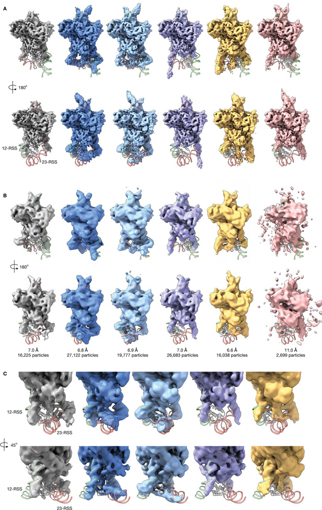
A) Front (top) and back (bottom) view of the six cryoDRGN density maps of the RAG complex from Figure 4B.

B) Density maps from 3D classification in cryoSPARC using the cryoDRGN density maps in (A) as initial models. Gold-standard FSC resolution and number of particles used in reconstruction are noted.

C) Two side views of the density maps from 3D classification in (B), focusing on the RSS and NBD.

Extended Data Figure 3. Missing head group of the Pf80S ribosome.

A) UMAP visualization of latent space encodings of EMPIAR-10028 particles with 50 sampled points shown in black. Sampled points are ordered according to distances in latent space (Methods). Visual inspection of the 50 volumes generated at the depicted points reveals 3 volumes with the 40S in a rotated state (purple) and 6 volumes with portions of the 40S head region missing (pink).

B) Density map of the 80S ribosome with the missing head group reconstructed by cryoDRGN (pink) compared with the density maps from Figure 4C showing the canonical (blue) and 40S-rotated (purple) forms of the 80S ribosome. The density maps are generated from points 32, 4, and 1 in panel A from left to right.

Extended Data Figure 4. Validation of Pf80S rotated state with cryoSPARC.

A) PCA and UMAP visualization of the cryoDRGN latent space representation of Pf80S particle images with 4,889 particles separated along PC1, selected with k-means clustering, colored in purple (Methods).

B) Density map from cryoSPARC homogeneous refinement (purple) using the 4,889 particles selected in (A). The density map is also shown superimposed with the cryoDRGN unrotated state (blue) and annotated as in Figure 4C.

C) Gold standard FSC (GSFSC) curve between independent half-maps of the cryoSPARC refinement of the Pf80S rotated state and map-to-map FSC between the cryoDRGN and cryoSPARC density map of the Pf80S rotated state. Dotted lines indicate 0.5 and 0.143 cutoffs.

Extended Data Figure 5. Filtering of particles from the assembling ribosome dataset.

A) UMAP visualization of the 10-D latent encodings from cryoDRGN as in Figure 5B, colored by cluster after fitting a 5-component Gaussian mixture model. The cluster that was removed from subsequent analysis is colored orange.

B) UMAP visualization of (A), colored by the magnitude of the latent encodings, ||z||.

C) Nine randomly sampled particle images from EMPIAR-10076 with latent encoding magnitude ||z|| > 10 as predicted from cryoDRGN training in (A,B). Each image is 419.2 Å along each side.

D) Table summarizing dataset filtering.

E,F) 2D classification and ab initio reconstruction of the 34,868 removed particles.

G,H) 2D classification and ab initio reconstruction of the 97,031 kept particles.

Extended Data Figure 6. Minor LSU assembly states reconstructed by cryoDRGN.

A) Density maps of the LSU minor assembly states reconstructed by cryoDRGN. Each cryoDRGN structure is generated at mean of the latent encoding of particles with the corresponding class assignment from Davis et al.¹²

B) Map-to-map FSC curves between the generated cryoDRGN density maps and the published density map from Davis et al.¹². Published resolutions for assembly states B-E ranged between ~4–5 Å. Dotted lines indicate 0.5 and 0.143 cutoffs.

C,D) Reproduction of the cryoDRGN latent space shown in Figure 5G, colored by minor assembly state (C), or viewed in separate panels (D).

Extended Data Figure 7. Validation of LSU class C4 with cryoSPARC.

A) Density map from cryoSPARC homogeneous refinement of the 1,113 particles selected from the cryoDRGN latent representation that constitute class C4 (right), compared with the density map generated by cryoDRGN (left) from Figure 5I. rRNA helix 68 is circled in red.

B) Gold standard FSC (GSFSC) curve between independent half-maps of the cryoSPARC reconstruction and map-to-map FSC between the cryoDRGN and cryoSPARC maps shown in (A). Dotted lines indicate 0.5 and 0.143 cutoffs.

Extended Data Figure 8. Reproducibility of cryoDRGN’s latent space representation of the assembling ribosome.

A) UMAP visualization of the latent encodings from replicate runs of cryoDRGN trained on the filtered particles of EMPIAR-10076. Particle embeddings are colored by major assembly state assigned from 3D classification in Davis et al¹².

B) UMAP visualization of (A), colored by cluster after fitting a 5-component Gaussian mixture model on the UMAP embeddings.

C, D) Consistency of the GMM labeling between replicates reported as the percentage of particles with identical labels (C) and the confusion matrix of GMM cluster assignments (D).

Extended Data Figure 9. Comparison of multi-body refinement and cryoDRGN of the pre-catalytic spliceosome.

A) Visualization of a rigid-body trajectory from multibody refinement of the pre-catalytic spliceosome. Snapshots are extracted from the trajectory along PC1 of rigid-body orientations, showing a large-scale motion of the SF3b subcomplex. The masks that define the rigid-body decomposition of the complex are shown on the right. The circle highlights a helix that breaks at the boundary between bodies where the rigid-body assumption no longer holds. Adapted from Video 3 of Nakane et al.¹⁹ and density maps and masks deposited in EMPIAR-10180.

B) Alternate view of cryoDRGN’s PC1 traversal in Figure 6. CryoDRGN learns the same overall motion of the SF3b subcomplex, however its neural network representation lacks the helix-breaking artifact.

Extended Data Figure 10. Comparison of cryoSPARC’s 3D variability analysis and cryoDRGN.

A) Density map of the consensus reconstruction and 2D projections of the top three 3DVA variability components (i.e. eigen-volumes) that form a linear basis describing structural heterogeneity of the pre-catalytic spliceosome.

B) 3DVA latent encodings of particles from the filtered EMPIAR-10180 dataset.

C) Comparison of 3DVA component 1 latent encodings and PC1 of the cryoDRGN 10-D latent encodings from Figure 6C. Correlation indicates Spearman correlation.

D) 3DVA component 1 trajectory at the depicted points in (B).

E) Alternate view of the density maps from the cryoDRGN PC1 trajectory in Figure 6D.

References

- 1.Nogales E. The development of cryo-EM into a mainstream structural biology technique. Nat. Methods 13, 24–27 (2015). [DOI] [PMC free article] [PubMed] [Google Scholar]
- 2.Cheng Y. Single-particle cryo-EM-How did it get here and where will it go. Science. 361, 876–880 (2018). [DOI] [PMC free article] [PubMed] [Google Scholar]
- 3.Bammes BE, Rochat RH, Jakana J, Chen D-H & Chiu W. Direct electron detection yields cryo-EM reconstructions at resolutions beyond 3/4 Nyquist frequency. J. Struct. Biol 177, 589–601 (2012). [DOI] [PMC free article] [PubMed] [Google Scholar]
- 4.Suloway C. et al. Automated molecular microscopy: The new Leginon system. J. Struct. Biol 151, 41–60 (2005). [DOI] [PubMed] [Google Scholar]
- 5.Li X. et al. Electron counting and beam-induced motion correction enable near-atomic-resolution single-particle cryo-EM. Nat. Methods 10, 584–590 (2013). [DOI] [PMC free article] [PubMed] [Google Scholar]
- 6.Zhang K. Gctf: Real-time CTF determination and correction. J. Struct. Biol 193, 1–12 (2016). [DOI] [PMC free article] [PubMed] [Google Scholar]
- 7.Brubaker MA, Punjani A. & Fleet DJ Building Proteins in a Day: Efficient 3D Molecular Reconstruction. Proc. IEEE Comput. Soc. Conf. Comput. Vis. Pattern Recognit, 3099–3108 (2015). [Google Scholar]
- 8.Scheres SHW A Bayesian view on cryo-EM structure determination. J. Mol. Biol 415, 406–418 (2012). [DOI] [PMC free article] [PubMed] [Google Scholar]
- 9.Bepler T. et al. Positive-unlabeled convolutional neural networks for particle picking in cryo-electron micrographs. Nat. Methods 16, 1153–1160 (2019). [DOI] [PMC free article] [PubMed] [Google Scholar]
- 10.Ahmed T, Yin Z. & Bhushan S. Cryo-EM structure of the large subunit of the spinach chloroplast ribosome. Sci. Rep 6, 1–13 (2016). [DOI] [PMC free article] [PubMed] [Google Scholar]
- 11.Wrapp D. et al. Cryo-EM structure of the 2019-nCoV spike in the prefusion conformation. Science. 367, 1260–1263 (2020). [DOI] [PMC free article] [PubMed] [Google Scholar]
- 12.Davis JH et al. Modular Assembly of the Bacterial Large Ribosomal Subunit. Cell 167, 1610−−1622.e15 (2016). [DOI] [PMC free article] [PubMed] [Google Scholar]
- 13.Haselbach D. et al. Structure and Conformational Dynamics of the Human Spliceosomal Bact Complex. Cell 172, 454−−464.e11 (2018). [DOI] [PubMed] [Google Scholar]
- 14.Sigworth FJ Principles of cryo-EM single-particle image processing. Microscopy (Oxf.) 65, 57–67 (2016). [DOI] [PMC free article] [PubMed] [Google Scholar]
- 15.Scheres SHW RELION: implementation of a Bayesian approach to cryo-EM structure determination. J. Struct. Biol 180, 519–530 (2012). [DOI] [PMC free article] [PubMed] [Google Scholar]
- 16.Punjani A, Rubinstein JL, Fleet DJ & Brubaker MA cryoSPARC: algorithms for rapid unsupervised cryo-EM structure determination. Nat. Methods 14, 290–296 (2017). [DOI] [PubMed] [Google Scholar]
- 17.Lyumkis D, Brilot AF, Theobald DL & Grigorieff N. Likelihood-based classification of cryo-EM images using FREALIGN. J. Struct. Biol 183, 377–388 (2013). [DOI] [PMC free article] [PubMed] [Google Scholar]
- 18.Grant T, Rohou A. & Grigorieff N. cisTEM, user-friendly software for single-particle image processing. Elife 7, e14874 (2018). [DOI] [PMC free article] [PubMed] [Google Scholar]
- 19.Nakane T, Kimanius D, Lindahl E. & Scheres SH Characterisation of molecular motions in cryo-EM single-particle data by multi-body refinement in RELION. Elife 7, e36861 (2018). [DOI] [PMC free article] [PubMed] [Google Scholar]
- 20.Liu W. & Frank J. Estimation of variance distribution in three-dimensional reconstruction I Theory. J. Opt. Soc. Am. A (1995) doi: 10.1364/josaa.12.002615. [DOI] [PubMed] [Google Scholar]
- 21.Penczek PA, Kimmel M. & Spahn CMT Identifying conformational states of macromolecules by eigen-analysis of resampled cryo-EM images. Structure 19, 1582–1590 (2011). [DOI] [PMC free article] [PubMed] [Google Scholar]
- 22.Tagare HD, Kucukelbir A, Sigworth FJ, Wang H. & Rao M. Directly reconstructing principal components of heterogeneous particles from cryo-EM images. J. Struct. Biol 191, 245–262 (2015). [DOI] [PMC free article] [PubMed] [Google Scholar]
- 23.Punjani A. & Fleet DJ 3D Variability Analysis: Directly resolving continuous flexibility and discrete heterogeneity from single particle cryo-EM images. bioRxiv 11, 2020.04.08.032466 (2020). [DOI] [PubMed] [Google Scholar]
- 24.Dashti A. et al. Trajectories of the ribosome as a Brownian nanomachine. Proc. Natl. Acad. Sci. U. S. A 111, 17492–17497 (2014). [DOI] [PMC free article] [PubMed] [Google Scholar]
- 25.Frank J. & Ourmazd A. Continuous changes in structure mapped by manifold embedding of single-particle data in cryo-EM. Methods 100, 61–67 (2016). [DOI] [PMC free article] [PubMed] [Google Scholar]
- 26.Moscovich A, Halevi A, Andén J. & Singer A. Cryo-EM reconstruction of continuous heterogeneity by Laplacian spectral volumes. Inverse Probl. (2020) doi: 10.1088/1361-6420/ab4f55. [DOI] [PMC free article] [PubMed] [Google Scholar]
- 27.Lederman RR & Singer A. Continuously heterogeneous hyper-objects in cryo-EM and 3-D movies of many temporal dimensions. arXiv 1704.02899 (2017). [Google Scholar]
- 28.Hornik K, Stinchcombe MB & White H. Multilayer feedforward networks are universal approximators. Neural Networks 2, 359–366 (1989). [Google Scholar]
- 29.Bracewell RN Strip Integration in Radio Astronomy. Aust. J. Phys 9, 198–217 (1956). [Google Scholar]
- 30.Kingma DP & Welling M. Auto-encoding variational bayes. in International Conference on Learning Representations, ICLR; (2014). [Google Scholar]
- 31.Ru H. et al. Molecular Mechanism of V(D)J Recombination from Synaptic RAG1-RAG2 Complex Structures. Cell 163, 1138–1152 (2015). [DOI] [PMC free article] [PubMed] [Google Scholar]
- 32.Wong W. et al. Cryo-EM structure of the Plasmodium falciparum 80S ribosome bound to the anti-protozoan drug emetine. Elife 3, e01963 (2014). [DOI] [PMC free article] [PubMed] [Google Scholar]
- 33.Ru H, Zhang P. & Wu H. Structural gymnastics of RAG-mediated DNA cleavage in V(D)J recombination. Current Opinion in Structural Biology (2018) doi: 10.1016/j.sbi.2018.11.001. [DOI] [PMC free article] [PubMed] [Google Scholar]
- 34.Sun M. et al. Dynamical features of the Plasmodium falciparum ribosome during translation. Nucleic Acids Res. (2015) doi: 10.1093/nar/gkv991. [DOI] [PMC free article] [PubMed] [Google Scholar]
- 35.McInnes L, Healy J. & Melville J. UMAP: Uniform Manifold Approximation and Projection for Dimension Reduction. arXiv 1802.03426 (2018). [Google Scholar]
- 36.Plaschka C, Lin P-C & Nagai K. Structure of a pre-catalytic spliceosome. Nature 546, 617–621 (2017). [DOI] [PMC free article] [PubMed] [Google Scholar]
- 37.Cormen TH, Leiserson CE, Rivest RL & Stein C. Introduction to Algorithms. in 595–601 (MIT Press and McGraw-Hill; ). [Google Scholar]
- 38.Zhang C, Bengio S, Hardt M, Recht B. & Vinyals O. Understanding deep learning requires rethinking generalization. Int. Conf. Learn. Represent. ICLR (2017). [Google Scholar]
- 39.Zivanov J, Nakane T. & Scheres SHW Estimation of high-order aberrations and anisotropic magnification from cryo-EM data sets in RELION-3.1. IUCrJ 7, 253–267 (2020). [DOI] [PMC free article] [PubMed] [Google Scholar]
- 40.Punjani A, Zhang H. & Fleet DJ Non-uniform refinement: Adaptive regularization improves single particle cryo-EM reconstruction. bioRxiv 179, 2019.12.15.877092 (2019). [DOI] [PubMed] [Google Scholar]
Methods-only References
- 41.Zhong ED, Bepler T, Davis JH & Berger B. Reconstructing continuous distributions of 3 D protein structure from cryo-EM images in International Conference of Learning Representations, ICLR (2020). [Google Scholar]
- 42.Bepler T, Zhong E, Kelley K, Brignole E. & Berger B. Explicitly disentangling image content from translation and rotation with spatial-VAE. in Advances in Neural Information Processing Systems (2019). [Google Scholar]
- 43.Vaswani A. et al. Attention is all you need. in Advances in Neural Information Processing Systems (2017). [Google Scholar]
- 44.Rezende DJ, Mohamed S. & Wierstra D. Stochastic backpropagation and approximate inference in deep generative models. in International Conference on Machine Learning, ICML (2014). [Google Scholar]
- 45.The PyMOL Molecular Graphics System, Version 2.3, Schrodinger, LLC. [Google Scholar]
- 46.Tang G. et al. EMAN2: an extensible image processing suite for electron microscopy. J. Struct. Biol 157, 38–46 (2007). [DOI] [PubMed] [Google Scholar]
- 47.Pettersen EF et al. UCSF Chimera - A visualization system for exploratory research and analysis. J. Comput. Chem 25, 1605–1612 (2004). [DOI] [PubMed] [Google Scholar]
- 48.Iudin A, Korir PK, Salavert-Torres J, Kleywegt GJ & Patwardhan A. EMPIAR: a public archive for raw electron microscopy image data. Nat. Methods 13, 387–388 (2016). [DOI] [PubMed] [Google Scholar]
- 49.Rosenthal PB & Henderson R. Optimal determination of particle orientation, absolute hand, and contrast loss in single-particle electron cryomicroscopy. J. Mol. Biol 333, 721–745 (2003). [DOI] [PubMed] [Google Scholar]
- 50.Pedregosa F. et al. Scikit-learn: Machine Learning in Python. J. Mach. Learn. Res 12, 2825–2830 (2011). [Google Scholar]
- 51.Goddard TD et al. UCSF ChimeraX: Meeting modern challenges in visualization and analysis. Protein Sci. 27, 14–25 (2018). [DOI] [PMC free article] [PubMed] [Google Scholar]
Associated Data
This section collects any data citations, data availability statements, or supplementary materials included in this article.
Supplementary Materials