Restricted Mean Survival Time as a Function of Restriction Time

Summary:

Restricted mean survival time (RMST) is a clinically interpretable and meaningful survival metric that has gained popularity in recent years. Several methods are available for regression modeling of RMST, most based on pseudo-observations or what is essentially an inverse-weighted complete-case analysis. No existing RMST regression method allows for the covariate effects to be expressed as functions over time. This is a considerable limitation, in light of the many hazard regression methods that do accommodate such effects. To address this void in the literature, we propose RMST methods that permit estimating time-varying effects. In particular, we propose an inference framework for directly modeling RMST as a continuous function of L. Large-sample properties are derived. Simulation studies are performed to evaluate the performance of the methods in finite sample sizes. The proposed framework is applied to kidney transplant data obtained from the Scientific Registry of Transplant Recipients (SRTR).

1. Introduction

For time to event data with right censoring, the proportional hazards model (Cox, 1972) has long been the default for conducting analysis requiring covariate adjustment. The principal summary measure that results from Cox regression is the hazard ratio (HR), which is routinely used to quantify between-group differences. This line of analysis relies on proportional hazards (PH), which is the assumption that the ratio of the two hazard functions are constant over time. Although the approach is convenient to implement, the PH assumption is frequently violated, leading to difficulties with interpretation (Struthers and Kalbfleisch, 1986; Wei and Schaubel, 2008).

A number of authors have advocated for using summary statistics beyond the hazard ratio in both clinical trials and observational data analyses, especially when the proportional hazards assumption has been called into doubt (Royston and Parmar, 2011; Schaubel and Wei, 2011; Royston and Parmar, 2013; Uno et al., 2014; Uno et al., 2015). In particular, the restricted mean survival time (RMST) has been suggested. Defined as the mean survival time up to a fixed time, L, in a given population, the RMST can simply be thought of as a L-year life expectancy. Mathematically, it is written as the area under the survival curve up to time L. First proposed in Irwin (1949), RMST was initially meant as a substitute for the overall mean, for settings where the presence of censoring prevented the estimation of the latter. More recently, it has come to be known as an interesting measure in its own right. Simulation studies have compared RMST treatment effect estimation and statistical power with HR-based tests both under proportional hazards and non-proportional hazards scenarios. Royston and Parmar (2013), Tian et al. (2017), and Huang and Kuan (2018) found that under PH scenarios, RMST-based and log-rank tests perform similarly (with a slight advantage for the log-rank test), while RMST performs better in non-PH scenarios. Hence, RMST is a clinically relevant and interpretable measure that does not depend on the PH assumption and requires little sacrifice in statistical power even when the PH assumption holds.

Most existing methods estimate RMST indirectly by integrating under an estimate of the survival curve. Irwin (1949) used the actuarial estimator for the survival probability and approximated the area under the curve using numerical quadrature methods. More recent methods that extend those of Irwin (1949) by incorporating covariates tend to proceed initially through hazard regression. Karrison (1987) introduced covariate adjustment for the RMST using a piece-wise exponential hazard model, assuming covariates affect the hazard in a multiplicative manner just as in the Cox model, subsequently obtaining the piecewise cumulative hazard, survival probability curve, and the restricted mean. Zucker (1998) followed a similar protocol, using a stratified Cox model instead. Even more recent approaches still require 4-5 sequential steps to obtain the restricted mean: estimate the regression parameter (e.g., through a Cox model); estimate the cumulative baseline hazard; transforming the subject-specific cumulative hazard, then integrate it to obtain the restricted mean (Chen and Tsiatis, 2001; Zhang and Schaubel, 2011). This process is cumbersome and computationally expensive in large data sets, especially to obtain asymptotic standard errors. Furthermore, through the use of Cox model, this process also relies on the proportional hazards assumption, which, if untrue, can also lead to bias, inefficient estimation, and a challenging interpretation.

Hence, several authors have suggested to directly model the RMST itself. Andersen et al. (2004) and Andersen and Pohar Perme (2010) used imputation based on pseudo-observations to model the RMST directly using generalized linear models. Tian et al. (2014) employed a different but similarly direct approach by constructing estimating equations for RMST based on Inverse Probability of Censoring Weighting (Robins and Rotnitzky, 1992; Robins, 1993; Robins and Finkelstein, 2000), similar to the approach of Zhao et al. for quality adjusted life (Zhao and Tsiatis, 1997; Zhao and Tsiatis, 1999). Wang and Schaubel (2018) employed a similar modeling strategy, but further extended the method to accommodate dependent censoring.

To the best of our knowledge, no existing regression methods have been proposed for modeling RMST as a continuous function of the restriction time, L. Zhao et al. 2016 make a strong case for by looking at the entire RMST curve, in order to obtain a complete temporal picture, much like the survival function. We extend this concept to the regression setting, which has two important analytic implications. First, through our proposed approach, one can obtain RMST predictions for various restriction times through a single model. Second and much more importantly, models fitted though our proposed methods yield time-varying covariate effects. The second property is essential for RMST regression to be on more equal footing with hazard regression, since the latter is currently the strong default analysis when time-varying covariate effects are an objective.

The remainder of this report is organized as follows. In Section 2, we describe the proposed methods, formulating the notation, data structure, and listing out the assumptions. In Section 3, we present the derived asymptotic properties. In Section 4, we present results from simulation studies to evaluate the accuracy of the proposed methods. In Section 5, we apply the method to the Scientific Registry of Transplant Recipients (SRTR) kidney transplant data, illustrating the use of our method. We conclude this report in Section 6 with a discussion. Asymptotic derivations are provided in the supporting information.

2. Proposed Methods

Let D_i be the survival time for subject i, where i = 1, …, n. Let C_i be the censoring time, assumed to be independent of D_i conditional on the baseline covariates. The observation time for subject i is X_i = D_i ∧ C_i, where a ∧ b = min{a, b}. The at-risk indicator is denoted by R_i(t) = I(X_i ⩾ t), and the event and censoring indicators are ${\Delta }_i^D=I\left(D_i⩽C_i\right)$ and ${\Delta }_i^C=I\left(C_i<D_i\right)$, respectively. We denote covariates predicting D_i and C_i by ${\mathit{Z}}_i^D$ and ${\mathit{Z}}_i^C$, respectively. Stacking these covariates and removing redundancy, we obtain Z_i. Our observed data are then given by $\left\{X_i,{\Delta }_i^D,{\Delta }_i^C,{\mathit{Z}}_i:i=1,\dots ,n\right\}$.

Let τ = max{X_i : i = 1, …, n} be the end of follow-up time, and L_max be a pre-specified maximal value of L after which estimation becomes potentially unstable and of little interest. Naturally, it is required that τ ⩾ L_max. Let L be a vector of length K where L = (L₁, L₂, …, L_K)′ values sorted in ascending order. For a particular element of L, say L_k, the restricted observation time is Y_ik = X_i ∧ L_k, and the corresponding observed-event indicator is Δ_ik = I(D_i ∧ L_k ⩽ C_i). Note that Δ_ik is analogous to a complete-case indicator, taking the value 1 if subject i either dies before (C_i ∧ L_k) or lives (and remains uncensored) past L_k.

In general, for any arbitrary value of L, we are interested in the average survival time up to L, modeled through an individual’s covariates:

$${\mu }_i\left(L\right):=E\left\{D_i\wedge L|{\mathit{Z}}_i^D\right\}.$$

As in Wang and Schaubel (2018), we assume the same direct relationship between the RMST and the baseline covariates. However, in addition, we assume that the covariate effects vary as a function of L in the following equation:

$$g\left[{\mu }_i\left(L\right)\right]\equiv g\left[E\left\{D_i\wedge L|{\mathit{Z}}_i^D\right\}\right]={{\mathit{\beta }}^{\prime }}_D\left(L\right){\mathit{Z}}_i^D,$$ (1)

where g is a strictly monotone link function with a continuous derivative within an open neighborhood ${\mathcal{B}}_D\left(L\right)$ of β_D(L). Some conventional examples of g(x) could be the identity link, log link, or logistic link. Without any adjustments, (1) is an infinite dimensional problem and would generally be inconvenient to estimate. Instead, we address the problem by assuming that β_D(L), a vector of continuous and monotonic functions, is able to be parametrically modeled as a function of L. For example, denote this parametric model of L as β_D(L) = α₀L₀(L) + … + α_mL_m(L), where L₀(L), L₁(L), …, L_m(L) are functions of L, i.e. parametric or spline functions. Let Z_i = (1, Z_i1, …, Z_ip)′ and L(L) = (L₀(L), L₁(L), …, L_m(L))′. Then we can re-express the covariate vector as follows:

$${\tilde{\mathit{Z}}}_i^D\left(L\right)={\mathit{Z}}_i\otimes \mathit{L}\left(L\right)$$

where ⊗ denotes the Kronecker product. Correspondingly, let α₀ = (α₀₀, …, α_0m)′, …, α_p = (α_p0, …, α_pm)′, such that the new parameter vector can be written as

$${\tilde{\mathit{\beta }}}_D=\left[\begin{array}{c}{\mathit{\alpha }}_0\\ {\mathit{\alpha }}_1\\ ⋮\\ {\mathit{\alpha }}_p\end{array}\right].$$

Hence, we can rewrite model (1) as:

$$g\left[{\mu }_i\left(L\right)\right]\equiv g\left[E\left\{D_i\wedge L|{\mathit{Z}}_i^D\right\}\right]={{\mathit{\beta }}^{\prime }}_D\left(L\right){\mathit{Z}}_i^D={\widetilde{{\mathit{\beta }}^{\prime }}}_D{\tilde{\mathit{Z}}}_i^D\left(L\right).$$ (2)

This parametrization in effect reduces an infinite dimensional problem to a finite dimensional one, thereby making it more convenient to estimate the regression parameter. The specific parametrization of α_k(L) requires careful consideration and should be supported by graphical evidence. For relationships that do not seem to be simply linear, the authors recommend fitting a spline as an initial choice. The knots of the spline should be pre-selected and evenly span across the represented data to ensure a comprehensive fit. Further exploration of this issue is given in Section 6.

Based on (2), in the absence of censoring, we can derive the following estimating equation:

$$\frac{1}{n}\sum _{i=1}^n\sum _{k=1}^K{\tilde{\mathit{Z}}}_i^D\left(L_k\right)\left[Y_{ik}-g^{-1}\left\{{\tilde{\mathit{\beta }}}^{\prime }{\tilde{\mathit{Z}}}_i^D\left(L_k\right)\right\}\right]=\mathbf{0}.$$ (3)

In effect, this is a stacked version of the estimating equation presented in Wang and Schaubel (2018), where each new iteration of the data (for each value of L_k) is stacked to make a complete vector of responses. Each individual is now represented in the data set K times through its relationship with individual L_ks. The complete response vector is then used to fit a model that incorporates each L_k as part of the covariate information. We then estimate the assumed model through generalized estimating equations (GEE). To retain flexibility and robustness, we utilize a working independence correlation structure for each individual.

As in most survival data, we are unlikely to observe D_i for all patients due to censoring. In this report, we will focus on independent censoring and make the standard assumption that C_i ⊥ D_i|Z_i. We further assume that the hazard for censoring time C_i follows a proportional hazards model (Cox, 1972),

$${\lambda }_i^C\left(t\right)={\lambda }_0^C\left(t\right)\exp \left({{\mathit{\beta }}^{\prime }}_C{\mathit{Z}}_i^C\right).$$ (4)

Then, each subject-specific cumulative hazards is given by ${\Lambda }_i^C\left(t\right)={\int }_0^t{\lambda }_i^C\left(u\right)du$ for i = 1, …, n. In the presence of censoring, $E\left({\tilde{\mathit{Z}}}_i^D\left(L_k\right)\left[Y_{ik}-g^{-1}\left\{{\tilde{\mathit{\beta }}}^{\prime }{\tilde{\mathit{Z}}}_i^D\left(L_k\right)\right\}\right]\right)\ne \mathit{0}$, but we can show that the IPCW weighted expectation $E\left({\tilde{\mathit{Z}}}_i^D\left(L_k\right){\Delta }_{ik}{W}_i^C\left(Y_{ik}\right)\left[Y_{ik}-g^{-1}\left\{{\tilde{\mathit{\beta }}}^{\prime }{\tilde{\mathit{Z}}}_i^D\left(L_k\right)\right\}\right]\right)$ has mean 0, where $W_i^C\left(t\right)=\exp \left\{{\Lambda }_i^C\left(t\right)\right\}$.

We then present the following estimating equation, proven in the supporting information to be unbiased for ${{\tilde{\mathit{\beta }}}^{\prime }}_D$ :

$${\mathbf{\Phi }}^{\ast }\left(\tilde{\mathit{\beta }}\right):=\frac{1}{n}\sum _{i=1}^n\sum _{k=1}^k{\tilde{\mathit{Z}}}_i^D\left(L_k\right){\Delta }_{ik}{W}_i^C\left(Y_{ik}\right)\left[Y_{ik}-g^{-1}\left\{{\tilde{\mathit{\beta }}}^{\prime }{\tilde{\mathit{Z}}}_i^D\left(L_k\right)\right\}\right]=0.$$ (5)

Because the cumulative censoring hazard is usually not known in real data settings, the following empirical estimating equation substitutes for ${\Lambda }_i^C\left(t\right)$ using the standard partial likelihood (Cox, 1975) and Breslow-Aalen (Breslow, 1972) estimator,

$$\mathbf{\Phi }\left(\tilde{\mathit{\beta }}\right):=\frac{1}{n}\sum _{i=1}^n\sum _{k=1}^K{\tilde{\mathit{Z}}}_i^D\left(L_k\right){\Delta }_{ik}{\widehat{W}}_i^C\left(Y_{ik}\right)\left[Y_{ik}-g^{-1}\left\{{\tilde{\mathit{\beta }}}^{\prime }{\tilde{\mathit{Z}}}_i^D\left(L_k\right)\right\}\right]=0.$$ (6)

The solution to (6) is shown to provide for consistent estimation of ${\tilde{\mathit{\beta }}}_D$; asymptotic properties are discussed in Section 3.

3. Asymptotic Properties

We specify the following regularity conditions (a)-(g):

1. $\left\{X_i,{\Delta }_i^D,{\Delta }_i^C,{\mathit{Z}}_i\right\}$, i = 1, 2, …, n are independently and identically distributed.

2. P{R_i(t) = 1} > 0 for t ∈ (0, τ), i = 1, …, n

3. |Z_ik| < M_Z < ∞ for i = 1, …, n, where Z_ik is the k^th component of Z_i

4. ${\Lambda }_i^C\left(\tau \right)<\infty$ and ${\Lambda }_i^C\left(t\right)$ is absolutely continuous for t ∈ (0, τ].

5. There exist neighborhoods ${\mathcal{B}}_C$ of β_C such that for k = 0, 1, 2,

   $$\underset{t\in \left(0,\tau \right],\mathit{\beta }\in {\mathit{\beta }}_C}{\sup }\Vert \frac{1}{n}\sum _{i=1}^n\exp \left({\mathit{\beta }}^{\prime }{\mathit{Z}}_i^C\right)R_i\left(t\right){\mathit{Z}}_i^{C\otimes k}-{\mathit{r}}_C^{\left(k\right)}\left(t;\mathit{\beta }\right)\Vert \stackrel{p}{\to }0,$$

   where v^⊗0 = 1, v^⊗1 = v, v^⊗2 = v′v, and

   $${\mathit{r}}_C^{\left(k\right)}\left(t;\mathit{\beta }\right)=E\left[\exp \left({\mathit{\beta }}^{\prime }{\mathit{Z}}_i^C\right)R_i\left(t\right){\mathit{Z}}_i^{C\otimes k}\right].$$

6. Define h(x) = ∂g⁻¹(x)/∂x, where h exists and is continuous in an open neighborhood ${\mathcal{B}}_D\left(L\right)$ of ${\tilde{\mathit{\beta }}}_D\left(L\right)$.

7. Matrices $\mathit{A}\left({\tilde{\beta }}_D\right)$, Ω_C(β_C) are both positive definite, and are defined below:

   $$\mathit{A}\left({\tilde{\mathit{\beta }}}_D\right)=E\left[\sum _{k=1}^K{\tilde{\mathit{Z}}}_i^D{\left(L_k\right)}^{\otimes 2}h\left\{{\widetilde{{\mathit{\beta }}^{\prime }}}_D{\tilde{\mathit{Z}}}_i^D\left(L_k\right)\right\}\right]$$

   $${\mathbf{\Omega }}_C\left({\mathit{\beta }}_C\right)=E\left[{\int }_0^{\tau }\left\{\frac{{\mathit{r}}_C^{\left(2\right)}\left(t;{\mathit{\beta }}_C\right)}{r_C^{\left(0\right)}\left(t;{\mathit{\beta }}_C\right)}-{\tilde{\mathit{z}}}_C{\left(t;{\mathit{\beta }}_C\right)}^{\otimes 2}\right\}d{N}_i^C\left(t\right)\right],$$

   where

   $${\tilde{\mathit{z}}}_C\left(t;\mathit{\beta }\right)=\frac{{\mathit{r}}_C^{\left(1\right)}\left(t;\mathit{\beta }\right)}{r_C^{\left(0\right)}\left(t;\mathit{\beta }\right)}.$$

Condition (a) could be relaxed, but additional technical developments would be needed to compensate. Condition (b) is required for identifiability. Conditions (c) - (f) are required for the convergence of stochastic integrals in several proofs. In (g), matrices $\mathit{A}\left({\tilde{\mathit{\beta }}}_D\right)$, Ω_C(β_C) are at least non-negative definite and will be positive-definite provided the covariate vectors are specified sensibly.

The main asymptotic results are presented below, in Theorems (1) and (2), with proofs presented in the supporting information.

Theorem 1: Under regularity conditions (a)-(g), as n → ∞, $\sqrt{n}\mathbf{\Phi }\left({\tilde{\mathit{\beta }}}_D\right)$ converges in distribution to a $\mathit{Normal}\left(\mathbf{0},\mathit{B}\left({\tilde{\mathit{\beta }}}_D\right)\right)$, where ${\mathit{B}}_i\left(\tilde{\mathit{\beta }}\right)={\sum }_{k=1}^K\left\{{\mathit{ϵ}}_{ik}\left(\tilde{\mathit{\beta }}\right)+{\mathbf{\Omega }}_C{\left({\mathit{\beta }}_C\right)}^{-1}{\mathit{U}}_i^C\left({\mathit{\beta }}_C\right){\mathit{K}}_C\left(\tilde{\mathit{\beta }}\right)\right\}$ and $\mathit{B}\left(\tilde{\mathit{\beta }}\right)\equiv E\left\{{\mathit{B}}_i{\left(\tilde{\mathit{\beta }}\right)}^{\otimes 2}\right\}$, where we define:

$${\mathit{ϵ}}_{ik}\left({\tilde{\mathit{\beta }}}_D\right)={\tilde{\mathit{Z}}}_i^D\left(L_k\right){\Delta }_{ik}{W}_i^C\left(Y_{ik}\right)\left[Y_{ik}-g^{-1}\left\{{\widetilde{{\mathit{\beta }}^{\prime }}}_D{\tilde{\mathit{Z}}}_i^D\left(L_k\right)\right\}\right]$$

$${\mathit{U}}_i^C\left({\mathit{\beta }}_C\right)={\int }_0^{\tau }\left\{{\mathit{Z}}_i^C-{\tilde{\mathit{z}}}_C\left(u;{\mathit{\beta }}_C\right)\right\}d{M}_i^C\left(u\right)$$

$${\mathit{D}}_i^C\left(t\right)={\int }_0^t\left\{{\mathit{Z}}_i^C-{\tilde{\mathit{z}}}_C\left(u;{\mathit{\beta }}_C\right)\right\}d{\Lambda }_i^C\left(u\right)$$

$${\mathit{K}}_C\left(\tilde{\mathit{\beta }}\right)\equiv E\left[{\mathit{ϵ}}_{ik}\left(\tilde{\mathit{\beta }}\right){\mathit{D}}_i^C{\left(Y_{ik}\right)}^{\prime }\right].$$

Proof of Theorem 1 uses results presented in Zhang and Schaubel (2011). Mainly, we borrow techniques for expressing the asymptotic empirical weight in terms of the true weight for independent censoring times. Theorem 1 sets the stage for the next theorem.

Theorem 2: Under regularity conditions (a)-(g), as n → ∞, ${\widehat{\mathit{\beta }}}_D$ converges in probability to ${\tilde{\mathit{\beta }}}_D$, and $\sqrt{n}\left({\widehat{\mathit{\beta }}}_D-{\tilde{\mathit{\beta }}}_D\right)$ converges in distribution to $\mathit{Normal}\left(0,\mathit{A}{\left({\tilde{\mathit{\beta }}}_D\right)}^{-1}\mathit{B}\left({\tilde{\mathit{\beta }}}_D\right)\mathit{A}{\left({\tilde{\mathit{\beta }}}_D\right)}^{-1}\right)$.

The proof of consistency follows from the use of the Inverse Function Theorem (Foutz, 1977). The asymptotic normality and variance follows from the combination of Theorem 1 and a sequence of Taylor expansions.

We propose a variance estimator that is computationally more convenient than that derived in Theorem 2. Specifically, the weight function is treated as known, such the middle matrix involves only ϵ_ik(β), which implies the following variance estimator,

$$\widehat{V}\left({\widehat{\mathit{\beta }}}_D\right)=\widehat{\mathit{A}}{\left({\tilde{\mathit{\beta }}}_D\right)}^{-1}{\widehat{\mathit{B}}}^{*}\left({\tilde{\mathit{\beta }}}_D\right)\widehat{\mathit{A}}{\left({\tilde{\mathit{\beta }}}_D\right)}^{-1},$$ (7)

where ${\widehat{\mathit{B}}}^{*}\left(\mathit{\beta }\right)=\widehat{E}\left\{{\left({\sum }_{k=1}^K{\mathit{ϵ}}_{ik}\left(\mathit{\beta }\right)\right)}^{\otimes 2}\right\}$. Treating the IPCW weights as fixed has a long history, dating back at least to the works of Robins et al. (2000). Moreover, Wang and Schaubel (2018) demonstrated through simulation that there was no practical difference between standard errors that treated the weights as fixed versus random. The asymptotic standard error (ASE) estimator given in (7) will be used in Sections 4 and 5. Computationally, (7) can be quickly computed with built-in commands in standard software (e.g., R, SAS), using any function that can handle weighted GEE data structures.

4. Simulation Study

For each subject, i = 1, …, n, we first generated a baseline covariate with two elements, Z_i = (Z_i1, Z_i2)′, with each element generated from a Unif(−1,1) distribution. The death time, D_i, was then generated from an exponential distribution with

$$E\left[D_i|{\mathit{Z}}_i\right]=g^{-1}\left({\alpha }_0+{\alpha }_1{Z}_{i1}+{\alpha }_2{Z}_{i2}\right).$$ (8)

Parameter settings were chosen to cover a wide variety of realistic scenarios. For g(x) = x, we set α = [4, 2.5, −2.5]′ for the ‘strong’ covariate effect scenario, and set α = [4, 0.75, −0.75]′ to represent weaker covariate effects. Note that Cox regression under the ‘strong’ scenario yields hazard ratios of HR₁ ≈ 0.45 and HR₁ ≈ 2.15 for Z_i1 and Z_i2, respectively; the ‘weak’ covariate setting lines up with HR₁ ≈ 0.80 and HR₂ ≈ 1.20. For g(x) = log(x), we set α = [1.25, log(2), −log(2)]′ and α = [1.25, log(1.25), −log(1.25)]′ for the strong and weak covariate effect scenarios, respectively. For the log link, the strong setting yields hazard ratios HR₁ ≈ 0.5 and HR₂ ≈ 2.0, while the weak setting corresponds to HR₁ ≈ 0.80 and HR₂ ≈ 1.25. Although we did not directly generate the restricted mean survival time D_i ∧ L, we can induce its relationship with the two covariates through Monte Carlo methods (with population size 10 million for each configuration).

With respect to censoring, we examined scenarios with a low (15% censored), moderate (30%) and high (45%) proportion censored. Independent censoring time, C_i, was generated from the following hazard,

$${\lambda }_i^C\left(t\right)={\lambda }_0^C\exp \left({\beta }_{C1}{Z}_{i1}+{\beta }_{C2}{Z}_{i2}\right).$$

For all settings, β_C1 = log(1.5) and β_C2 = −log(1.5). We varied ${\lambda }_0^C$ in order to generate the desired percent censored; censoring parameters are given in the table captions.

We present the results for sample size n = 1000, under low, moderate and high censoring scenarios. For each setting, 500 iterates were generated. In Tables 1 and 2, we present results for the strong covariate setting for the linear and log links, respectively. For illustrative purposes, we will select L = {5, 7.5, 10}. Tables 1 and 2 contain the true values, bias, empirical standard deviation (ESD), the asymptotic standard error (ASE), and empirical coverage probabilities (CP) corresponding to the asymptotic 95% confidence intervals.

Table 1.

Simulation results: linear link, strong covariate effect. Data were generated using β_D = [4, 2.5, −2.5]. True β_D are given by [2.621, 1.006, −1.006] for L = 5, [3.140, 1.440, −1.440] for L = 7.5, and [3.453, 1.753, −1.756] for L = 10. For low censoring (15%), ${\lambda }_0^C=0.025$, β_C = [−log(1.5), log(1.5)]. For moderate censoring (30%), ${\lambda }_0^C=0.1$, β_C = [−log(1.5), log(1.5)]. For high censoring (45%), ${\lambda }_0^C=0.225$, β_C = [−log(1.5), log(1.5)].

L	Censor %	Parameter	BIAS	ESD	ASE	CP
5	15	β 0	−0.001	0.053	0.055	0.960
		β 1	−0.004	0.098	0.095	0.944
		β 2	−0.009	0.100	0.095	0.940
	30	β 0	−0.003	0.056	0.062	0.976
		β 1	0.004	0.101	0.106	0.958
		β 2	0.003	0.107	0.106	0.942
	45	β 0	−0.002	0.064	0.079	0.982
		β 1	−0.004	0.121	0.131	0.964
		β 2	−0.001	0.123	0.132	0.956
7.5	15	β 0	−0.005	0.073	0.078	0.964
		β 1	−0.011	0.138	0.136	0.944
		β 2	−0.008	0.141	0.136	0.958
	30	β 0	−0.009	0.081	0.094	0.974
		β 1	−0.003	0.145	0.160	0.964
		β 2	0.009	0.160	0.160	0.944
	45	β 0	−0.009	0.099	0.133	0.988
		β 1	−0.017	0.194	0.220	0.974
		β 2	0.003	0.195	0.220	0.968
10	15	β 0	−0.005	0.089	0.097	0.968
		β 1	−0.009	0.170	0.171	0.950
		β 2	−0.009	0.173	0.170	0.964
	30	β 0	−0.011	0.104	0.124	0.970
		β 1	−0.005	0.197	0.213	0.978
		β 2	0.008	0.210	0.211	0.954
	45	β 0	−0.016	0.132	0.197	0.992
		β 1	−0.037	0.290	0.323	0.982
		β 2	−0.011	0.287	0.323	0.964

Table 2.

Simulation results: log link, strong covariate effect. Data were generated using β_D = [1.25, log(2), −log(2)]. True β_D are given by [0.923, 0.359, −0.359] for L = 5, [1.074, 0.451, −0.451] for L = 7.5, and [1.148, 0.515, −0.515] for L = 10. For low censoring (15%), ${\lambda }_0^C=0.025$, β_C = [−log(1.5), log(1.5)]. For moderate censoring (30%), ${\lambda }_0^C=0.1$, β_C = [−log(1.5), log(1.5)]. For high censoring (45%), ${\lambda }_0^C=0.225$, β_C = [−log(1.5), log(1.5)].

L	Censor %	Parameter	BIAS	ESD	ASE	CP
5	15	β 0	−0.001	0.022	0.023	0.946
		β 1	0.001	0.035	0.036	0.956
		β 2	−0.004	0.034	0.036	0.964
	30	β 0	−0.001	0.023	0.026	0.974
		β 1	0.001	0.041	0.041	0.956
		β 2	0.001	0.037	0.041	0.974
	45	β 0	−0.001	0.028	0.034	0.986
		β 1	0.001	0.047	0.053	0.978
		β 2	−0.001	0.050	0.054	0.958
7.5	15	β 0	−0.003	0.026	0.027	0.952
		β 1	0.000	0.041	0.043	0.948
		β 2	−0.004	0.041	0.043	0.954
	30	β 0	−0.002	0.028	0.033	0.970
		β 1	0.002	0.049	0.051	0.974
		β 2	0.005	0.046	0.051	0.968
	45	β 0	−0.005	0.039	0.048	0.980
		β 1	0.004	0.066	0.073	0.960
		β 2	0.002	0.072	0.074	0.960
10	15	β 0	−0.003	0.029	0.029	0.956
		β 1	−0.000	0.045	0.048	0.962
		β 2	−0.005	0.047	0.048	0.948
	30	β 0	−0.001	0.031	0.039	0.976
		β 1	0.003	0.058	0.061	0.966
		β 2	0.007	0.056	0.061	0.956
	45	β 0	−0.008	0.052	0.062	0.966
		β 1	0.006	0.089	0.093	0.956
		β 2	0.001	0.096	0.095	0.952

The general conclusion from Tables 1 and 2 is that, in moderate samples, the proposed estimator is approximately unbiased. Furthermore, the ESDs matched the ASEs very closely, supporting the accuracy of the derivations, and that treating the inverse probability censoring weights as known is adequate for maintaining estimation accuracy of the standard errors. The empirical coverage probabilities are similarly very close to the nominal level.

Figure 1 displays plots comparing $\widehat{\mathit{\beta }}(L)$ with β(L) from the 30% censoring scenario shown in Table 1. The proposed estimator is quite accurate across all L values plotted, as evidenced by the fact that ‘estimated’ and ‘true’ lines are practically indistinguishable.

Figure 1.

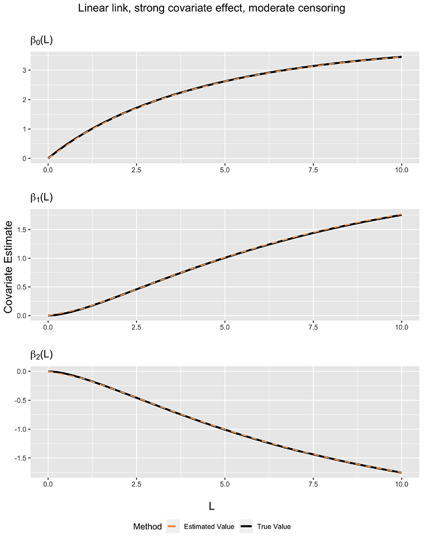
Comparison between true covariate values and estimated covariate values as a function of L for linear link. Data were generated using β_D = [4, 2.5, −2.5]. Censoring was generated at 30%, with ${\lambda }_0^C=0.1$, β_C = [−log(1.5), log(1.5)].

Additional simulation results are provided in the supporting information. In particular, we show results for weak covariate effects in Web Tables 1–2. Results are very similar those afore-described for Tables 1–2. We show results for smaller sample sizes (n = 500 and n = 250) in Web Tables 3–4. Results are acceptable, although residual bias is greater than that shown in Tables 1–2, and CP is a bit lower, as one would expect. In Web Tables 5–6, we compare the efficiency of the proposed methods with that of Wang and Schaubel (2018); efficiency is shown to be approximately equal for the two approaches. Finally, we evaluated the impact of increasing the number of k values (i.e., the number of stacked data sets) in Web Tables 7–8. It appears that slight gains in efficiency can be achieved by increasing K.

5. Analysis of Kidney Transplantation Data

We applied our proposed method to estimating time to graft failure in kidney-transplantation recipients. The data were obtained from the Scientific Registry of Transplant Recipients (SRTR). The SRTR data system includes data on all donors, wait-listed candidates and transplant recipients in the U.S., as submitted by members of the Organ Procurement and Transplantation Network (OPTN), and has been described elsewhere. The Health Resources and Services Administration (HRSA), U.S. Department of Health and Human Services provides oversight to the activities of the OPTN and SRTR contractors.

The study population includes end stage renal disease patients who received a kidney transplant between January 01, 2000 and December 31, 2014. For this analysis, we included only those who received deceased donor kidneys, excluded all recipients younger than 18 years of age and those who have received a previous kidney transplants. Graft failure, our main event of interest, is defined as the minimum of death, transplant failure (return to dialysis), and re-transplantation. This is consistent with the majority of previous kidney transplant literature (Zhong et al., 2019). Each patient was followed from the date of transplant to the earliest of graft failure or censoring date, or the end of observation period of December 31, 2014. Independent censoring occurred through a loss of follow-up or administrative censoring. For this analysis, a total of n = 127, 082 patients were included in the study population. A total of 45, 516 (35.8%) patients experienced graft failure. Of these, 48.6% of them died, 50.6% experienced transplant failure, and 0.8% had a re-transplant.

To illustrate our method, we chose a set of five baseline recipient covariates: age, gender, height, weight, and log of the kidney donor recipient index (log-KDRI) (Rao et al., 2009). Age, height, weight, and log-KDRI are continuous, while gender is binary. We selected our L = [1, 2, 3, …, 10]′ years. In this case, the L_max is set to be 10 years. The data were replicated and assorted into an expanded dataset, with Y_ik = Y_i ∧ L_k, k = 1, 2, …, 10. The same L was also used to fit the model, using individual L′_ks as knots in the parametric spline. Although we opted to use the same vector both to create the expanded data set as well as to fit the parametric spline model, the two could be chosen separately if desired.

In Figure 2, we plot time-varying effects for some of the more prominent covariates. Due to our having shifted continuous covariates, the intercept (top left panel) pertains to a 40-year old male who is 170cm tall, weighs 80kg, receives a kidney transplant from a deceased donor with KDRI=1, which is approximately the 25th percentile of donor quality, per Zhong et al. (2019).

Figure 2.

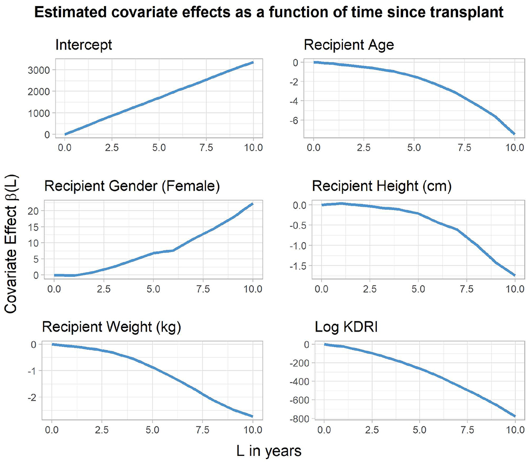
Analysis of SRTR data: Estimated covariate effects as a function of time since transplant.

We chose here to use the linear link for ease of interpretability, but other link functions could also be used if desired. To find ${\widehat{\beta }}_{Z_k}\left(L\right)$ for a particular covariate Z_k using this spline parametrization, we follow the following formula:

$${\widehat{\beta }}_{Z_k}\left(L\right)={\widehat{\alpha }}_{k0}L+{\widehat{\alpha }}_{k1}{\left(L-1\right)}_{+}+{\widehat{\alpha }}_{k2}{\left(L-2\right)}_{+}+{\widehat{\alpha }}_{k3}{\left(L-3\right)}_{+}+{\widehat{\alpha }}_{k4}{\left(L-4\right)}_{+}+{\widehat{\alpha }}_{k5}{\left(L-5\right)}_{+}+{\widehat{\alpha }}_{k6}{\left(L-6\right)}_{+}+{\widehat{\alpha }}_{k7}{\left(L-7\right)}_{+}+{\widehat{\alpha }}_{k8}{\left(L-8\right)}_{+}+{\widehat{\alpha }}_{k9}{\left(L-9\right)}_{+},$$

where a₊ = max{a, 0}.

Similarly, we can obtain $\widehat{V}\left\{{\widehat{\beta }}_{Z_k}\left(L\right)\right\}$ by requesting the standard robust variance-covariance matrix from GEE software/functions. Since the spline terms are constant (zero variance), one can simply obtain the variance using relevant elements in the variance-covariance matrix and summing through the sum of variance formula.

In Figure 3 we present RMST predictions for various covariate patterns. Covariate sets 1 and 3 represent lower-risk patients, while 2 and 4 correspond to patients that are higher-risk. Contrasts between the predicted RMST values across patients generally become more pronounced as L increases. Note that, due to the use of spline terms, this pattern is not forced by the model. Covariate sets, represented by different colors, appears in color in the electronic version of this article, and any mention of color refers to that version.

Figure 3.

Predicted RMST projections by covariate pattern and time. Covariate Set 1 refers to a 65 year old female who received an organ with KDRI of 0.75. Covariate Set 2 is a 45 year old female who received an organ with KDRI of 1.35. Covariate Set 3 refers to a 30 year old male who received an organ with KDRI of 0.75. Covariate Set 4 refers to a 40 year old male who received an organ with KDRI of 1.5. All recipients were assumed to be 170cm in height and 80kg in weight. This figure appears in color in the electronic version of this article, and any mention of color refers to that version.

6. Discussion

In this report, we developed a method for modeling restricted mean survival time as a function of the restriction time. Unlike existing methods, the proposed methods allow covariate effects to depend on restriction time. The methods also permit the analyst to obtain RMST predictions for several time horizons through a single model. Our method requires specifying a maximum ‘reasonable’ restriction time, L_max, after which RMST is then modeled as a parametric function of L on (0, L_max]. Our method amounts to developing a “super-model”, through stacking data sets defined by L_k values which map out a grid over (0, L_max]. Through our methods, one can create a flexible and temporal picture of covariate effects as a function of L. The proposed variance estimator is convenient to implement and was shown to work well in moderate samples. Furthermore, computational feasibility in larger data sets is implied by our method having easily been able to handle national organ transplant registry data.

The proposed methods allow the covariate effects to depend on time, which is a major advantage over Wang and Schaubel (2018). The flexibility to use time-varying effects is well-accepted and frequently utilized in the context of hazard regression. Moreover, the work of Zhao et al. (2016) underscores the importance of viewing RMST as a function of restriction time in comparing groups nonparametrically. The major advantage of our work over Zhao et al. is that our proposed methods utilize regression, while Zhao et al. (2016) uses nonparametric comparisons. Zhao et al. (2018) would generally not be applicable to observational studies requiring simultaneous estimation of many predictors and/or when some predictors are continuous; e.g., the transplant registry study we analyzed in Section 5.

The proposed methods require IPCW, which is generally known to be subject to instability. It should be noted that small remaining-uncensored probabilities are less of an issue in RMST modeling, provided that a sensible value of L (or, in our case, L_max) is chosen. It is not necessary to compute the weight function too far into the tail of the observation time distribution, hence avoiding scenarios where there are very few subjects remaining at-risk (which leads to large and unstable weights). We illustrate this phenomenon in Web Figure 1, which shows box plots of the IPCW weight function versus L for the SRTR data analyzed in Section 5. The plot reveals that variability in the weight function increases as L increases, as does the maximum weight. However, unrealistically large weights are not observed, as the maximum weight observed is 27 at L = 10, and the vast majority of weights at L = 10 were less than three, which is very reasonable for a dataset with sample size of 127,082. In the event that unduly large weights did occur, one could cap the weight function.

In addition to choosing L_max, the two other main decisions involved in our method are the vector components of L used to create the expanded data-set, and the precise parametric model (including specification of knots, if appropriate) used to fit the expanded data-set. In our experience, for the first question, it is generally important to create a well spread out grid that includes copies of the data both smaller and larger than L’s of interest. For the second question, we propose that investigators fit separate models at a grid of L values to preliminarily determine the functional form of covariate effects and use that as a guide to determine the specific parametrization. For example, in the SRTR data set, it was clear after this step that a simple linear model would be deficient. On both of these topics, further research would help elucidate the pros and cons of particular approaches.

Finally, to illustrate our method, we applied it to kidney transplantation data to study post-transplant outcomes. To our knowledge, this is the first paper to provide a temporal model of RMST in the kidney transplantation setting.

References

- Andersen PK, Hansen MG, and Klein JP (2004). Regression analysis of restricted mean survival time based on pseudo-observations. Lifetime data analysis, 10, 335–350. [DOI] [PubMed] [Google Scholar]
- Andersen PK and Pohar Perme M (2010). Pseudo-observations in survival analysis. Statistical methods in medical research, 19, 71–99. [DOI] [PubMed] [Google Scholar]
- Breslow NE (1972). Contribution to discussion of papeer by dr cox. J. Roy. Statist. Assoc., B, 34, 216–217. [Google Scholar]
- Chen P-Y and Tsiatis AA (2001). Causal inference on the difference of the restricted mean lifetime between two groups. Biometrics, 57, 1030–1038. [DOI] [PubMed] [Google Scholar]
- Cox DR (1972). Regression models and life-tables. Journal of the Royal Statistical Society. Series B (Methodological), 34, 187–220. [Google Scholar]
- Cox DR (1975). Partial likelihood. Biometrika, 62, 269–276. [Google Scholar]
- Foutz RV (1977). On the unique consistent solution to the likelihood equations. Journal of the American Statistical Association, 72, 147–148. [Google Scholar]
- Huang B and Kuan P-F (2018). Comparison of the restricted mean survival time with the hazard ratio in superiority trials with a time-to-event end point. Pharmaceutical statistics, 17, 202–213. [DOI] [PubMed] [Google Scholar]
- Irwin J (1949). The standard error of an estimate of expectation of life, with special reference to expectation of tumourless life in experiments with mice. The Journal of hygiene, 47, 188. [DOI] [PMC free article] [PubMed] [Google Scholar]
- Karrison T (1987). Restricted mean life with adjustment for covariates. Journal of the American Statistical Association, 82, 1169–1176. [Google Scholar]
- Rao PS, Schaubel DE, Guidinger MK, Andreoni KA, Wolfe RA, Merion RM, Port FK, and Sung RS (2009). A comprehensive risk quantification score for deceased donor kidneys: the kidney donor risk index. Transplantation, 88, 231–236. [DOI] [PubMed] [Google Scholar]
- Robins J and Rotnitzky A (1992). Recovery of information and adjustment for dependent censoring using surrogate markers. In Jewell N, Dietz K, and Farewell V, editors, AIDS Epidemiology, pages 297–331. Birkhäuser Boston. [Google Scholar]
- Robins JM (1993). Information recovery and bias adjustment in proportional hazards regression analysis of randomized trials using surrogate markers,. In Proceedings of the Biopharmaceutical Section, American Statistical Association, volume 24, page 3. San Francisco CA. [Google Scholar]
- Robins JM and Finkelstein DM (2000). Correcting for noncompliance and dependent censoring in an aids clinical trial with inverse probability of censoring weighted (ipcw) log-rank tests. Biometrics, pages 779–788. [DOI] [PubMed] [Google Scholar]
- Royston P and Parmar MK (2011). The use of restricted mean survival time to estimate the treatment effect in randomized clinical trials when the proportional hazards assumption is in doubt. Statistics in medicine, 30, 2409–2421. [DOI] [PubMed] [Google Scholar]
- Royston P and Parmar MK (2013). Restricted mean survival time: an alternative to the hazard ratio for the design and analysis of randomized trials with a time-to-event outcome. BMC medical research methodology, 13, 152. [DOI] [PMC free article] [PubMed] [Google Scholar]
- Schaubel DE and Wei G (2011). Double inverse-weighted estimation of cumulative treatment effects under nonproportional hazards and dependent censoring. Biometrics, 67, 29–38. [DOI] [PMC free article] [PubMed] [Google Scholar]
- Struthers CA and Kalbfleisch JD (1986). Misspecified proportional hazard models. Biometrika, 73, 363–369. [Google Scholar]
- Tian L, Fu H, Ruberg SJ, Uno H, and Wei L-J (2017). Efficiency of two sample tests via the restricted mean survival time for analyzing event time observations. Biometrics, [DOI] [PMC free article] [PubMed] [Google Scholar]
- Tian L, Zhao L, and Wei L (2014). Predicting the restricted mean event time with the subject’s baseline covariates in survival analysis. Biostatistics, 15, 222–233. [DOI] [PMC free article] [PubMed] [Google Scholar]
- Uno H, Claggett B, Tian L, Inoue E, Gallo P, Miyata T, Schrag D, Takeuchi M, Uyama Y, Zhao L, et al. (2014). Moving beyond the hazard ratio in quantifying the between-group difference in survival analysis. Journal of clinical Oncology, 32, 2380. [DOI] [PMC free article] [PubMed] [Google Scholar]
- Uno H, Wittes J, Fu H, Solomon SD, Claggett B, Tian L, Cai T, Pfeffer MA, Evans SR, and Wei L-J (2015). Alternatives to hazard ratios for comparing the efficacy or safety of therapies in noninferiority studies. Annals of internal medicine, 163, 127–134. [DOI] [PMC free article] [PubMed] [Google Scholar]
- Wang X and Schaubel DE (2018). Modeling restricted mean survival time under general censoring mechanisms. Lifetime data analysis, 24, 176–199. [DOI] [PMC free article] [PubMed] [Google Scholar]
- Wei G and Schaubel DE (2008). Estimating cumulative treatment effects in the presence of nonproportional hazards. Biometrics, 64, 724–732. [DOI] [PubMed] [Google Scholar]
- Zhang M and Schaubel DE (2011). Estimating differences in restricted mean lifetime using observational data subject to dependent censoring. Biometrics, 67, 740–749. [DOI] [PMC free article] [PubMed] [Google Scholar]
- Zhao H and Tsiatis AA (1997). A consistent estimator for the distribution of quality adjusted survival time. Biometrika, 84, 339–348. [Google Scholar]
- Zhao H and Tsiatis AA (1999). Efficient estimation of the distribution of quality-adjusted survival time. Biometrics, 55, 1101–1107. [DOI] [PubMed] [Google Scholar]
- Zhao L, Claggett B, Tian L, Uno H, Pfeffer MA, Solomon SD, Trippa L, and Wei L (2016). On the restricted mean survival time curve in survival analysis. Biometrics, 72, 215–221. [DOI] [PMC free article] [PubMed] [Google Scholar]
- Zhong Y, Schaubel DE, Kalbfleisch JD, Ashby VB, Rao P, and Sung RS (2019). Reevaluation of the kidney donor risk index. Transplantation, 103, 1714–1721. [DOI] [PMC free article] [PubMed] [Google Scholar]
- Zucker DM (1998). Restricted mean life with covariates: modification and extension of a useful survival analysis method. Journal of the American Statistical Association, 93, 702–709. [Google Scholar]
Associated Data
This section collects any data citations, data availability statements, or supplementary materials included in this article.