Abstract
Rising medical costs are an emerging challenge in policy decisions and resource allocation planning. When cumulative medical cost is the outcome, right-censoring induces informative missingness due to heterogeneity in cost accumulation rates across subjects. Inverse-weighting approaches have been developed to address the challenge of informative cost trajectories in mean cost estimation, though these approaches generally ignore post-baseline treatment changes. In post-hysterectomy endometrial cancer patients, data from a linked database of Medicare records and the Surveillance, Epidemiology, and End Results program of the National Cancer Institute reveal substantial within-subject variation in treatment over time. In such a setting, the utility of existing intent-to-treat approaches is generally limited. Estimates of population mean cost under a hypothetical time-varying treatment regime can better assist with resource allocation when planning for a treatment policy change; such estimates must inherently take time-dependent treatment and confounding into account. In this paper, we develop a nested g-computation approach to cost analysis to address this challenge, while accounting for censoring. We develop a procedure to evaluate sensitivity to departures from baseline treatment ignorability. We further conduct a variety of simulations and apply our nested g-computation procedure to two-year costs from endometrial cancer patients.
1. INTRODUCTION
Cancers of the endometrium comprise approximately 92% of cancers of the uterine body or corpus; it was estimated that nearly sixty-thousand new cases of endometrial cancer would be diagnosed in the U.S. in 2018 and over ten-thousand died from cancers of the uterine body (American Cancer Society, 2018). Current policy changes enacted by the U.S. government through the Medicare Access and CHIP Reauthorization Act (2015) and the Quality Payment Program (2017) have stimulated payers and health care providers alike to develop new reimbursement plans based not merely on the provision of service, but on potential successes and failures incurred by the patients and providers. While the overarching principle is to provide the best care possible for less cost, the act of determining overall cost for the past and the future remains the immediate goal. Given the recent rise in medical costs, studies to estimate mean medical costs in endometrial cancer patients are of value for budgeting and planning purposes (Papanicolas et al., 2018; Dieleman et al., 2017). In the ideal case, such studies would include data on lifetime post-intervention medical costs; this is generally impractical, so prior studies in other disease areas have identified cumulative cost until either death or some fixed bound on time—whichever comes first—as a suitable outcome measure, thus creating three categories of participants: (1) those who die prior to the fixed upper bound on time and hence have complete cost outcomes observed, (2) those for whom their censoring time occurs after the upper bound and hence have complete cost data, and (3) those for whom their censoring time occurs prior to the upper bound and hence have incomplete cost data (Herridge et al., 2011; Liao et al., 2006).
Incomplete follow-up data poses subtle challenges in analyzing cost outcomes. When a subject’s survival time is censored, so too is her cumulative cost outcome. Well understood approaches such as the Kaplan-Meier method and the Cox proportional hazards model, despite their utility when seeking to account for right-censoring in time-to-event data, are not appropriate when the outcome of interest is cumulative cost. Due to the heterogeneous nature of cost accumulation across individuals, the cumulative cost at the time of censoring is generally not independent of the theoretical total cost over the fixed time interval of interest, even if the censoring time is itself completely independent of the time to death or study completion (illustrated in Figure 1). We refer to this challenge as one of informative cost trajectories. Because of this challenge, analyzing medical cost as if a time-to-event measure is therefore a fundamentally flawed strategy.
Figure 1:
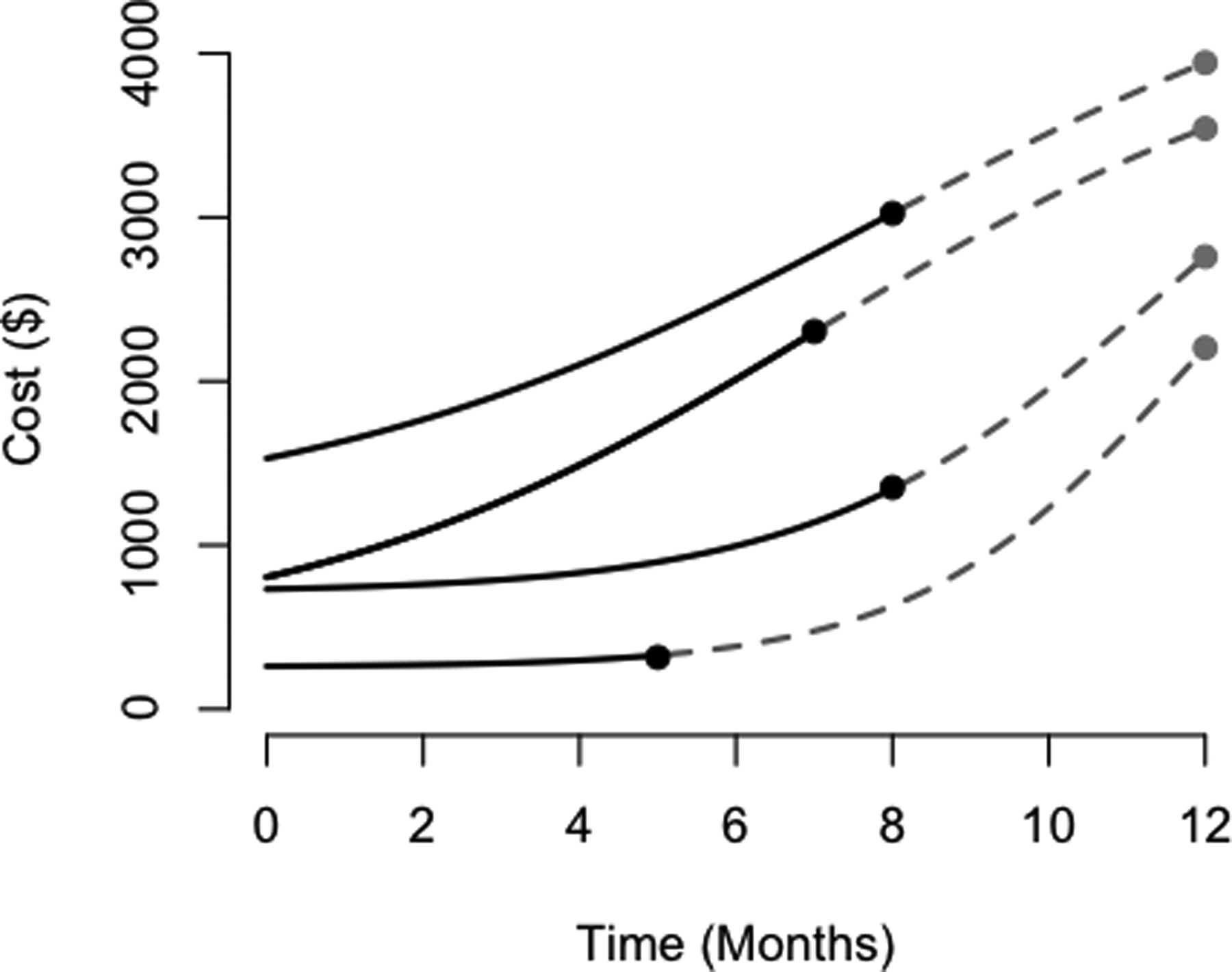
Here, we illustrate informative cost trajectories; in particular, cumulative costs at time of censoring are correlated with theoretical cumulative cost over one year, despite the censoring times being generated independently of the cost outcome (for each of these trajectories, the time range of interest is a constant twelve months for all patients, and hence the time of censoring is uncorrelated with the total time of interest). Observed portions of cost trajectories are plotted over time as solid black curves for censored individuals until their time of censoring. The hypothetical remainder of their trajectories are plotted as dashed gray curves until the time of study completion. The curves in this figure do not cross for ease of demonstration, though they may cross in practice.
Recognizing this challenge, Lin et al. (1997) proposed an estimator for mean costs, expressed as a sum of products of the Kaplan-Meier estimator for death/survival and suitable estimators for mean costs within defined time intervals. Bang and Tsiatis (2000) altered this estimator such that desirable asymptotic properties could be achieved under weaker assumptions, whereby mean costs are estimated within discrete intervals using inverse probability-of-censoring weights based on the Kaplan-Meier estimator. This method was then broadened by Lin (2000, 2003) to compare costs across levels of a predictor of interest, such as treatment. Johnson and Tsiatis further consider the setting of variable (and potentially informatively censored) treatment duration (2004; 2005). Li et al. (2016) proposed the inclusion of inverse probability-of-treatment weights (IPTW) as one of several ways to address measured confounding, and further improved upon existing methods by adopting a super learner algorithm to accommodate complex cost distributions. Other common statistical challenges encountered when modeling cost outcomes include handling zero-costs, right-skewness, and censoring; these can be addressed using a variety of regression and likelihood approaches.
Previously developed approaches only consider treatment at a single time and are therefore intent-to-treat in nature. Current considerations in endometrial cancer motivate the formal development of approaches to account for within-subject variation in treatment. Endometrial cancers are ordinarily treated initally with surgery (e.g., hysterectomy); depending upon other factors, adjuvant radiation or chemotherapy may be a component of treatment in the months following surgery (American Cancer Society, 2016). Emerging insights into a patient’s care over time (e.g., comorbidity measures) will bring forth modifications to her treatment plan in a fashion that is in keeping with concurrent best practices. Since a patient’s cumulative medical cost is influenced by treatment previously received, changes in treatment obscure our ability to easily estimate the monetary resources that would need to be allocated to endometrial cancer patients. Namely, consideration of baseline treatment is insufficient for this purpose.
Based on the linked database of Medicare records and the Surveillance, Epidemiology, and End Results program of the National Cancer Institute (henceforth referred to as the SEER-Medicare data), treatment modifications are fairly common over the first two years post-hysterectomy (Figure 2). Existing approaches to estimate mean cumulative cost using these data estimate mean costs conditional on baseline treatment status and would, in effect, disregard post-baseline treatment modifications. Since, for instance, only 10% of women in the SEER-Medicare data receiving chemotherapy within the first two years following surgery actually receive it within the first month, the practical relevance of such an estimand remains dubious. Instead, it would be of broader clinical interest to estimate a parameter that better aligns with a proposed policy change (i.e., the population mean cost post-surgery in the hypothetical setting where all patients receive a particular treatment). In the wake of an emerging policy change, such an estimate would be of great assistance for resource allocation, whereas an ad hoc modifications to approaches considering only baseline treatment status would most likely not. For instance, to retroactively consider a patient who is treated at any time as if she were treated at baseline could result in substantial bias. Existing approaches further presume censoring times are non-informative of death times conditional on observed baseline covariates, rather than time-updated covariates. Such strict assumptions regarding the censoring mechanism can pose further serious limitations to the interpretability of results.
Figure 2:
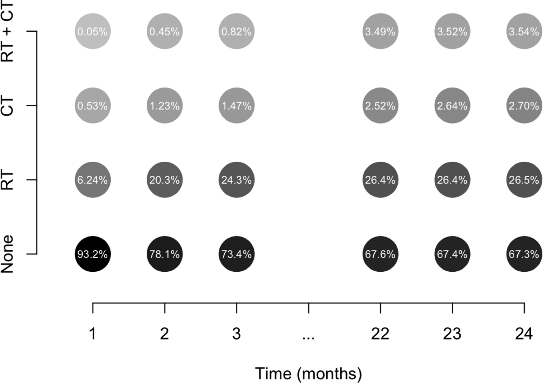
Illustration of treatment changes in SEER-Medicare data of women with confirmed endometrial cancer. In these data, once someone is treated, she is considered a treated patient for the remainder of the time on study. During each month, a subgroup of untreated individuals go on to receive chemotherapy (CT) and/or radiation (RT). Other subgroups of individuals having previously received one treatment go on to receive the other (RT + CT). Darker shading is used to denote higher relative frequency within a particular month.
This manuscript focuses on the development of methodology to elucidate mean costs under longitudinal (non-dynamic) treatment regimes in the real-world setting of time-dependent treatment and confounding. In the development of these methods, we also seek to accommodate the challenges of time-updating risks of censoring and death. We base this work on the g-formula and g-computation, a framework used to estimate marginal means under entire time-dependent treatment regimes. (Robins, 1986; Neugebauer et al., 2006; Snowden et al., 2011). The parametric g-formula has been increasingly employed in various clinical areas in recent years to address time-dependent treatment and confounding (Cole et al., 2013; Taubman et al., 2009; Young et al., 2011; Westreich et al., 2012). Previously, we introduced the idea of g-computation to illustrate the difference between intention-to-treat and as-treated causal effects in cost settings (Spieker et al., 2018). In this paper, we develop what we refer to as the “nested g-formula” to handle outcomes like cumulative cost that are sums of repeated measures that themselves serve as time-dependent confounders of longitudinal treatment. As will be made apparent in the sections that follow, it will be necessary to modify the g-formula to admit reasonable assumptions regarding censoring and death. In addition, we develop a sensitivity analysis for departures from the ignorability assumption; carry out simulation studies to assess the performance of the method; and we carry out a thorough data analysis of the endometrial cancer data set.
The remainder of this paper is organized as follows. In Section 2, we motivate the challenges associated with estimating population-mean costs with time-dependent treatment and confounding when there is censoring and death. In Section 3, we present our nested g-computation approach to address these challenges in the analysis of cost data with repeated outcome measures. We also develop a procedure to evaluate sensitivity of results to departures from the assumption of treatment assignment ignorability at baseline. In Section 4, we empirically compare the nested g-formula to existing approaches and evaluate the sensitivity of our model to departures from primary main assumptions, focusing on misspecification of the cost model. In Section 5, we apply the developed methods to cost outcomes on women with endometrial cancer from the SEER-Medicare data set. We focus in this section on sensitivity to departures from major assumptions. We conclude with a discussion of findings, including study limitations and potential future directions.
2. REAL-WORLD CHALLENGES IN LONGITUDINAL COST DATA
In this manuscript, the primary target of inference involves marginal, population-mean costs under hypothetical user-specified time-varying treatment regimes. We first lay out the notation of the manuscript; we then explain the real-world barriers to estimating the target parameter in longitudinal studies of cumulative cost with censoring.
Let i = 1, … , N index study subjects, and let j = 1, … , J index equally spaced intervals over the time range of interest [0, τ]: 0 ≡ τ0 < ⋯ < τJ ≡ τ. Let Aj and Lj denote treatment status (e.g., radiation therapy) and confounders (e.g., comorbidity index and cancer stage) at the start of interval j, respectively, and let Yj denote cost in interval j. In turn, let denote cumulative cost over [0, τ]. We use overbar notation to denote variable history (e.g., and . Analogously, we let Aj = (Aj, … , AJ), for instance. We adopt the potential outcomes notation of Rubin (1978), extended by Robins (1986) to permit time-varying treatment and confounders. Let denote the set of all possible treatment regimes, and the potential cost under treatment . Likewise, let denote the potential confounder under treatment . The target of inference, , can be described as the mean cost over [0, τ] under the hypothetical setting in which the treatment were set to the value ; identification requires a nonzero probability that the censoring time exceeds time τ, as noted by Lin (2000).
In practice, intermediate costs are influenced by prior treatment status, and in turn influence future treatment choices. That cumulative costs are only partially observed for censored patients is therefore a meaningful barrier to the goal of estimating the population mean of interest, especially (but not only) if the censoring mechanism is related to observed variables. Figure 3 presents a directed acyclic graph (DAG) in order to illustrate the nature of time-dependent treatment and confounding with cumulative cost over three time intervals as the outcome, with the challenge of censoring in mind.
Figure 3:
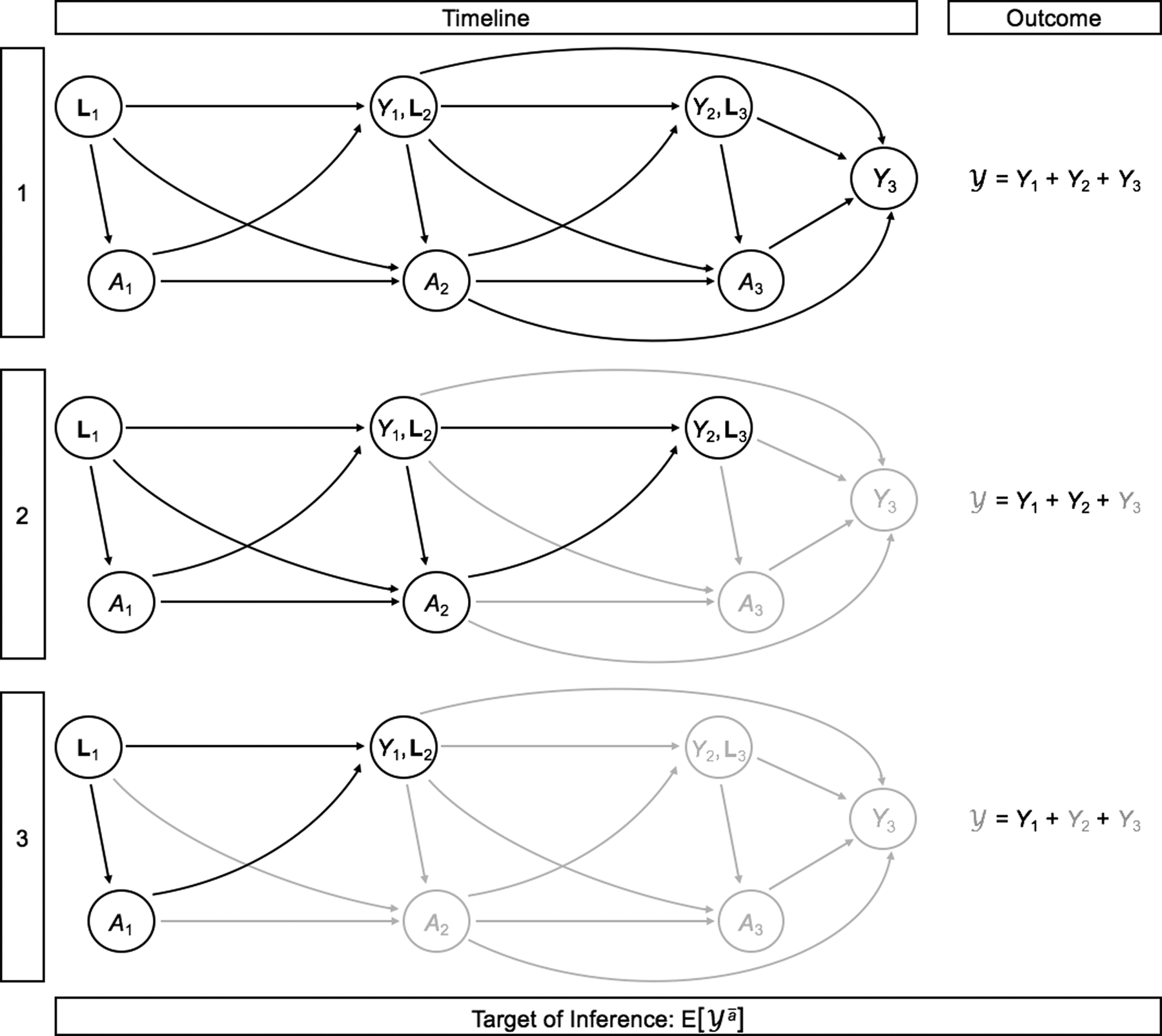
Illustration of censoring in longitudinal studies of cumulative cost with time-dependent treatment and confounding. For simplicity, we illustrate this in the setting of J = 3 time points. Observed variables are shown in black; after censoring, unobserved variables are shown in gray. The outcome is only completely observed for patient 1, but not for patients 2 and 3 as they are censored after their second and first observations, respectively.
G-computation was developed by Robins (1986) to address time-dependent treatment and confounding when estimating marginal means. Therefore, the g-computation framework seems well suited for the problem of estimating mean costs. Issues surrounding censoring of sums of intermediate outcomes demand the formulation of more explicit assumptions and will involve some procedural departures from Robins’ original approach. Additionally, in certain disease settings (such as cancers), death may occur prior to time τ in a fashion that is not completely random, further complicating estimation of . When a patient dies prior to censoring, her cumulative cost outcome is observed, though we need to be careful in defining, interpreting, and estimating this target parameter. By setting treatment to , we do not suggest that we are interested in the mean cost in the hypothetical setting under which all patients are alive over [0, τ] to receive treatment in its entirety. Rather, we seek to target the mean cost in the hypothetical scenario in which all patients receive treatment for as long as they actually would survive under that treatment. This distinction will become extremely important in formulating assumptions (Section 3).
3. THE NESTED G-FORMULA FOR COST
Daniel et al. (2013) provide a tutorial on g-computation and how it relates to alternative causal approaches. We refer the reader to this work for an introduction to the g-formula and its assumptions. As noted in Section 2, we must formulate additional assumptions specific to cost. We formalize the necessary identifying assumptions for in Section 3.1, and introduce the nested g-formula together with an associated Monte-Carlo integration technique for estimation in Section 3.2. In Section 3.3, we then formalize an approach to evaluate the sensitivity of estimation to departures from the assumption of no unmeasured confounding at baseline (i.e., ignorability of baseline treatment assignment).
3.1. Notation and assumptions
Let Cj denote censoring status at the start of interval j, and Dj death during interval j. We assume that for j′ > j (that is, no cost is accumulated after death). Further let denote the observed interval of death or study completion, whichever comes first; will denote its potential value under treatment assignment . We make the following identification assumptions:
No interference: (the potential cost history is not influenced by the treatment assignment of others).
Sequential consistency: (observed cost, confounder, and death history are equal to their respective potential values under a treatment regime that assigns each participant their observed treatment history).
Positivity: (each potential treatment regime has nonzero probability of occurrence irrespective of covariate history).
Sequentially ignorable treatment: (no unmeasured confounding; also known as “exchangeability”).
Sequentially ignorable censoring: (censoring is conditionally independent of the potential costs).
Conditionally non-informative censoring: (censoring is conditionally independent of death).
The latter two assumptions are similar to ignorable treatment, and are a key component of identifying the target of inference, , on the basis of observed data.
3.2. The nested g-formula
The original g-formula, appropriate for a single outcome measured at the end of the study, is an expression for a marginal mean formulated by sequentially invoking the tower property of expectation in reverse temporal order. Importantly, since a cumulative cost outcome, , can be represented as the sum of interval costs (see Section 2), a similar construction can be invoked in this setting within each single interval; that is, can be represented by treating analogously to the prior confounders, Lj. Hence, we let Wj = (Yj−1, Lj) for ease of notation, and let any variable with a subscript of zero be, by convention, zero. By convention, suppose that for j′ > j. Under the identifying assumptions, we can derive a suitable expression for the mean potential cost in interval j:
| (1) |
| (2) |
By linearity of expectation, , where the expression for is given above. We refer to this as the nested g-formula, and the process of its estimation as nested g-computation (the target parameter can be realized as sequential iteration of the g-formula, whereby in each iteration the previous outcomes and death are treated as confounders).
Ignorability of treatment assignment allows us to plug treatment regime into this expression; treatment assignment is not modeled at any stage. The sequentially ignorable censoring assumption allows us to handle censoring analogously by plugging in Cj = 0 ∀j. Therefore, uncensored individuals contribute to estimation of the target parameter for as many observations as they are not censored. To clarify, death is an absorbing state that stops the accrual of data and accumulation of further cost. Hence, plugging in Dj = 0 would target the mean cost under treatment in the hypothetical setting where everyone in the population survives through the interval [0, τ]; this is not the approach we take. In our motivating example of endometrial cancer, it is of greater real-world relevance to consider the marginal mean cost under treatment in the hypothetical setting where the population is indeed uncensored through the interval [0, τ], but the individuals of that population survive for as long as they would under the treatment . In order to target the latter parameter, we marginalize over the distribution of death at each time, accommodating systematic variation in the risk thereof.
If all variables are discrete and there are sufficient data in each category, an estimate can be obtained nonparametrically; however, such a setting is ordinarily not realistic. One will often make parametric assumptions about the distribution of Yj, Lj, and Dj. Markov-type assumptions are common in the parametric g-formula to limit computational burden. Monte-Carlo integration can be used to evaluate the integral at hand, whereby data are repeatedly simulated under estimated models, plugging in treatment . Under assumptions (1)-(6), the random draws estimate the marginal distribution of potential cost outcomes, . Given a sufficiently large number of random draws, those simulated potential outcomes can be averaged, thereby numerically solving the high-dimensional integral of the nested g-formula. No general closed-form analytic expression exists for the variance of ; the nonparametric bootstrap instead can be employed to estimate standard errors, construct confidence intervals, and conduct inference (Davison and Hinkley, 1997).
Algorithm 1 below describes how to perform nested g-computation for estimation of using a model-based approach under a Markov property such that Yj and Lj are influenced only by previously measured variables occurring in the concurrent or previous time interval. By convention, assume that no individuals are censored at the start of the first interval (C1 = 0), and let R denote the (sufficiently large) number of g-computation iterations:

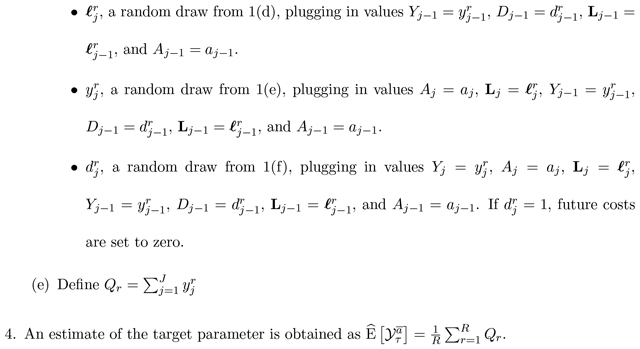
The nonparametric bootstrap can be employed by creating B full-sized data-sets of N individuals (re-sampled from the original data, with replacement), and repeating Steps (1)–(4) on the B full-sized data sets. From the B resulting estimates, standard errors can be computed and confidence intervals formed.
3.3. A sensitivity analysis procedure for violations to baseline ignorability
We now focus on challenges associated with the assumption of treatment assignment ignorability. This can be realized as the union of two assumptions: (1) , and (2) , for j ≥ 2. In observational data, the former of these assumptions, henceforth referred to as ignorability of baseline treatment assignment, should be examined closely as many pre-baseline factors available to the individuals choosing an initial treatment are unavailable in the data. Should any of these factors serve as a cause of higher cost, the assumption of baseline treatment assignment ignorability is violated. We therefore propose a procedure to evaluate sensitivity to departures from ignorability of baseline treatment, but when the remainder of assumptions are satisfied, including post-baseline ignorability of treatment assignment.
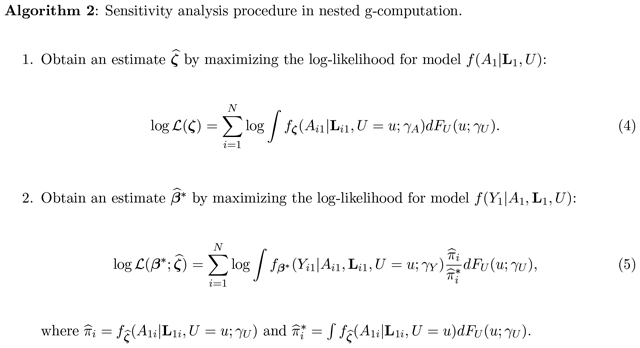
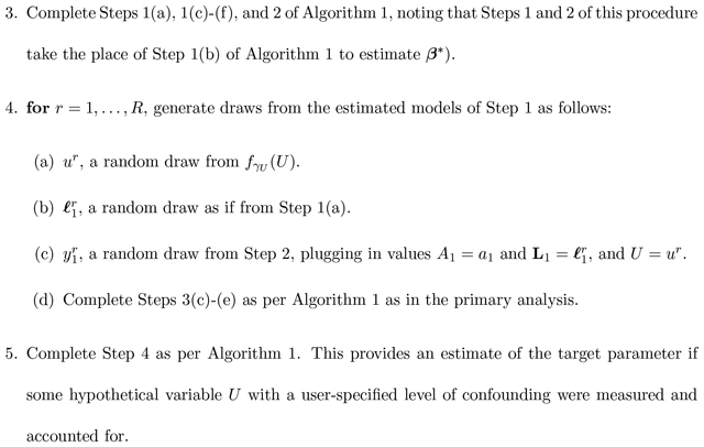
Suppose there is some univariate unmeasured U for which baseline ignorability of treatment assignment holds when considered together with L1 (in other words, suppose that ). It would be of interest to obtain an estimate of as it would be under proposed levels of confounding strength had U actually been measured and accounted for. Suppose we invoke a first-order Markov assumption under which each variable can only be directly influenced by variables in the concurrent and prior interval. In a primary analysis under which all assumptions are assumed satisfied, nested g-computation involves the modeling stage (fitting a series of baseline models for L1, Y1, D1, and follow-up models for Lj, Yj, and Dj), and the Monte-Carlo integration stage (simulating data from those models sequentially with set to ).
If we imagine some unmeasured U of a particular level of confounding strength, we would want to generate draws of Y1 from a model conditional not just on L1 and A1, but also on U in the Monte-Carlo integration stage. To do this, we would need to simulate from an estimated model that conditions not only on L1 and A1, but also on U. Because the parameters of these two models are potentially distinct, we will index them by β* and β, respectively. We will refer to the respective likelihoods as the conditional and marginal likelihoods (keeping in mind that the terms refer specifically to whether we are conditioning on U or not; both models condition on A1 and L1). For simplicity, we focus our attention on scenarios in which U ⫫ L1, though we do not assume that U ⫫ L1|A1 as per Lin et al (1998). Under a proposed distribution for U, we may derive a likelihood for the conditional parameter β* solely in terms of observed data, and of course, any and all user-specified sensitivity parameters γ:
| (3) |
If U is binary, the integral can be evaluated easily as a sum. In such a case, the complete sensitivity parameter vector γ comprises three classes of sensitivity parameters (SPs), described as follows: γU = P(U = 1) (the prevalence of U in the population), γA (the effect of U on A1, conditional on L1), and γY (the effect of U on Y1, conditional on L1 and A1). Here, ζ is a nuisance parameter that need not be estimated simultaneously with . To conduct an analysis to evaluate sensitivity to departures from ignorability of baseline treatment, one must obtain an estimate of β* from the marginal likelihood of (3). Then, the Monte-Carlo integration procedure would involve simulating from the conditional models at baseline (together with any sensitivity parameters), and then proceeding normally for follow-up intervals.
Algorithm 2 describes the sensitivity analysis procedure to evaluate the impact of departures from baseline ignorability. Let γU denote the sensitivity parameter(s) that describe FU(u). Let γA denote the user-specified sensitivity parameter(s) describing the impact of U on A1. Let γY denote the user-specified sensitivity parameter(s) describing the impact of U on Y1.
4. SIMULATION STUDY
We conduct a set of simulation studies in order to assess the finite-sample performance of the nested g-formula under a binary time-varying treatment. In all simulations, we set N = 2,000 subjects and J = 6 observations; we use Ng = 50,000 iterations for the Monte-Carlo integration procedure and B = 500 bootstrap replicates. Moreover, we invoke a first-order Markov assumption for simplicity, such that each variable can only be influenced by variables in the concurrent interval and the interval prior. We further use a single normally distributed time-varying confounder (e.g., a transformed propensity score, as per Lu (2005)). We seek to understand performance under varied levels of censoring, varied treatment generating mechanisms, and different cost-outcome mechanisms (both under correct specification and misspecification).
In all simulations, we consider two treatment generation scenarios (TGS). In the first TGS, we consider treatment as generated randomly at each interval and in a fashion dependent upon prior variables, and we consider the following two comparator regimes: never treated and always treated . In the second TGS, we consider treatment to be absorbing, such that once a patient is treated, he or she is considered treated for the remainder of the study; we consider three comparator treatment regimes: never treated , commencing treatment halfway through the study (, and always treated . All study subjects are presumed uncensored at the study’s start. The censoring rate at each follow-up time depends upon previous covariates. We consider, in each case, a low censoring rate (approximately 5% censored by the end of the sixth and final time point), and a moderate censoring rate (approximately 23%).
We conduct four sets of simulations: one under correct cost model specification and three under some form of misspecification. In the first two sets, cost outcomes follow a zero-inflated homoscedastic log-normal distribution. We fit a correctly specified cost model in the first set; in the second set, we instead fit a zero-inflated Gamma model to the data. In the third set of simulations, data are generated under a zero-inflated heteroscedastic log-normal model in which the cost variance at each time depends upon the concurrent confounder and treatment status; the cost data are incorrectly modeled as if homoscedastic. In the fourth set of simulations, we generate cost outcomes from a mixture of zero-inflated log-normal models, with a 0.02 probability of a very high intercept. Further specific details about the parameters of the simulation studies are provided in Online Appendix A.
Table 1 presents results from the first set of simulations, under correct specification. The estimates obtained from our nested g-computation show little bias, and standard errors closely match the empirical repeat-sample standard errors. Table 2 presents results from the second set of simulations, under which the costs are generated from a zero-inflated log-normal process and the (misspecified) zero-inflated Gamma cost model is used in the nested g-formula. Under these simulation parameters, the levels of bias are comparably low under this form of misspecification, and the bootstrap standard errors demonstrate robustness to this form of misspecification.
Table 1:
Simulation results (Set 1): Correctly specified zero-inflated log-normal cost model. Depicted are the true means in each scenario (in hundreds of dollars), the average estimate across simulations, the empirical standard error across Monte-Carlo replications, and the average estimated bootstrap standard error.
| TGS | Regime | True Mean | Low Censoring | Moderate Censoring | ||||
|---|---|---|---|---|---|---|---|---|
| Est. | SE | Est. | SE | |||||
| 1 | 10.1 | 10.2 | 0.167 | 0.168 | 10.2 | 0.200 | 0.204 | |
| 1 | 12.3 | 12.4 | 0.172 | 0.173 | 12.4 | 0.219 | 0.223 | |
| 2 | 10.1 | 10.2 | 0.139 | 0.150 | 10.2 | 0.160 | 0.175 | |
| 2 | 11.0 | 11.0 | 0.119 | 0.121 | 11.0 | 0.138 | 0.145 | |
| 2 | 12.3 | 12.4 | 0.237 | 0.241 | 12.4 | 0.283 | 0.284 | |
Table 2:
Simulation results (Set 2): Incorrectly specified zero-inflated Gamma cost model (the true data generating mechanism is zero-inflated log-normal). Depicted are the true means in each scenario (in hundreds of dollars), the average estimate across simulations, the empirical standard error across Monte-Carlo replications, and the average estimated bootstrap standard error.
| TGS | Regime | True Mean | Low Censoring | Moderate Censoring | ||||
|---|---|---|---|---|---|---|---|---|
| Est. | SE | Est. | SE | |||||
| 1 | 10.1 | 10.2 | 0.183 | 0.173 | 10.2 | 0.222 | 0.210 | |
| 1 | 12.3 | 12.4 | 0.178 | 0.179 | 12.4 | 0.240 | 0.231 | |
| 2 | 10.1 | 10.2 | 0.209 | 0.213 | 10.2 | 0.228 | 0.247 | |
| 2 | 11.0 | 11.0 | 0.145 | 0.155 | 11.0 | 0.171 | 0.181 | |
| 2 | 12.3 | 12.4 | 0.157 | 0.152 | 12.4 | 0.201 | 0.196 | |
Table 3 presents results from the third set of simulations, under which the costs are generated from a zero-inflated heteroscedastic log-normal process, but in which homoscedasticity is incorrectly assumed in the nested g-formula. Here, we see an increase in absolute bias, with an upward bias for treatment regimes involving no treatment , and downward for the other treatment regimes. The bootstrap standard errors demonstrate robustness to this form of misspecification.
Table 3:
Simulation results (Set 3): Incorrectly specified zero-inflated homoscedastic log-normal cost model (the true data generating mechanism incorporates heteroscedasticity). Depicted are the true means in each scenario (in hundreds of dollars), the average estimate across simulations, the empirical standard error across Monte-Carlo replications, and the average estimated bootstrap standard error.
| TGS | Regime | True Mean | Low Censoring | Moderate Censoring | ||||
|---|---|---|---|---|---|---|---|---|
| Est. | SE | Est. | SE | |||||
| 1 | 10.1 | 10.5 | 0.179 | 0.178 | 10.4 | 0.208 | 0.213 | |
| 1 | 13.4 | 12.7 | 0.201 | 0.204 | 12.7 | 0.252 | 0.262 | |
| 2 | 10.1 | 10.4 | 0.152 | 0.155 | 10.3 | 0.178 | 0.181 | |
| 2 | 11.5 | 11.2 | 0.129 | 0.134 | 11.1 | 0.155 | 0.162 | |
| 2 | 13.4 | 12.7 | 0.266 | 0.289 | 12.6 | 0.316 | 0.331 | |
Table 4 presents results from the third set of simulations, under which the log-normal positive costs are generated from with a mixture of intercepts with two components, but in which this mixture is unaccounted for in the nested g-formula and a single intercept is modeled. The average estimates across simulations are close to the true means, and bootstrap standard errors again approximate the empirical repeat-sample standard errors across simulations.
Table 4:
Simulation results (Set 4): Incorrectly specified zero-inflated log-normal cost model (the true data generating mechanism incorporates a 2% probability of a very high cost). Depicted are the true means in each scenario (in hundreds of dollars), the average estimate across simulations, the empirical standard error across Monte-Carlo replications, and the average estimated bootstrap standard error.
| TGS | Regime | True Mean | Low Censoring | Moderate Censoring | ||||
|---|---|---|---|---|---|---|---|---|
| Est. | SE | Est. | SE | |||||
| 1 | 11.3 | 11.1 | 0.166 | 0.163 | 11.1 | 0.194 | 0.196 | |
| 1 | 13.4 | 13.4 | 0.282 | 0.301 | 13.4 | 0.339 | 0.368 | |
| 2 | 11.3 | 11.1 | 0.167 | 0.176 | 11.1 | 0.203 | 0.207 | |
| 2 | 12.2 | 12.1 | 0.140 | 0.143 | 12.1 | 0.166 | 0.173 | |
| 2 | 13.4 | 13.4 | 0.256 | 0.273 | 13.5 | 0.304 | 0.325 | |
5. APPLICATION TO SEER-MEDICARE DATA
We apply the nested g-computation approach to our motivating example of Stage I and II endometrial cancer patients from the SEER-Medicare linked database. Using these data, we seek to estimate mean two-year cost under a number of hypothetical post-hysterectomy adjuvant treatment strategies. Information on N = 13,722 women with endometrial cancer as confirmed by hysterectomy were available from the SEER-Medicare data, with cases diagnosed between 2000 and 2011 (follow-up through 2013). Monthly costs were aggregated for each patient for a period of two years post-surgery. By the time of study completion, there were 626 observed deaths and 714 observed censoring events prior to two-years (the remaining 12,382 subjects were observed for the two-year duration). Treatment assignment was considered as two binary variables within each month: an indicator of any current or prior adjuvant radiation therapy (RT), and an indicator of any current or prior adjuvant chemotherapy (CT); that is, treatment was considered in a monotone fashion from the time of surgery to the end of the two-year period or until death, whichever comes first. Of note, the positivity assumption of Section 3.1 can be relaxed to accommodate this treatment definition. In particular, letting and denote the RT and CT status at time j, respectively, the positivity assumptions can be expressed as and ; by definition, and . During the first month, 864 women underwent RT, and 80 underwent CT. Among the 13,008 uncensored subjects in the twenty-fourth month, 3,759 had received or were undergoing RT and 782 had received or were undergoing CT.
The following were considered as potential confounders: age of diagnosis, baseline FIGO cancer stage (IA, IB, I NOS, II, and II NOS), race category (White, Black, and Other), time-varying Charlson Comorbidity Index (CCI), and number of hospitalizations in the prior month (from Month 2 onwards). To handle the data sparsity in CCI and number of prior hospitalizations, we re-categorized these variables as 0, 1, 2, or ≥ 3.
In the nested g-computation models, we invoke the Markov assumption described in our simulations. We believe this simplification is justified in large part because medical costs at a given time are more strongly associated with recent treatments as compared to treatment more distant in time; if much of the information from residual time-dependent confounding owing to earlier treatment status is captured by the time-varying covariates appearing in the models, we would expect bias to be low. The empirical joint distribution of the baseline covariates was used in place of parametric models. The joint distribution of the baseline confounders was specified as follows. Baseline cost was modeled using a (two-part) zero-inflated log-normal model. The first component modeled the odds of a zero cost using logistic regression, conditioning on all baseline confounders and categorical treatment; the second component modeled the cost as log-normal, conditional on a positive cost, and again conditional on baseline confounders and categorical treatment. The number of hospitalizations in the first month was modeled conditional on all prior confounders, but further adjusting for an indicator of zero cost in the first month and log cost in the first month (zero costs are mapped to a log cost of zero). No participants died during the first interval.
The joint distribution of the confounders at follow-up was specified by multinomial models, adjusting for all confounders in the prior interval, including a term for the indicator of a zero cost in the prior months, adjusting for log prior cost, and prior categorical treatment. The cost at follow-up was modeled with a two-part zero-inflated log-normal, adjusting for concurrent and prior confounders, additionally including a term for the indicator of a zero cost in the prior months, adjusting for log prior cost, and prior categorical treatment. The odds of death during each follow-up interval was modeled using logistic regression, adjusting for confounders and cost in the concurrent and prior intervals. All age and log-cost adjustments were performed using cubic splines with knots at their respective first and second tertiles (70 and 76 years for age, 8.96 and 9.37 for baseline log-cost, and 4.04 and 6.09 for post-baseline log-cost). Parameters from each proposed model were estimated and used for the Monte-Carlo integration procedure (coefficient estimates from each of the fitted models can be found in Online Appendix B).
In order to evaluate the goodness-of-fit, we plotted the fitted values against the standardized residuals (Figure 4) for the first interval and follow-up intervals. The residuals appear to be approximately of mean zero across the levels of the fitted values. The figures additionally provide evidence of heteroscedasticity across the levels of the fitted values.
Figure 4:
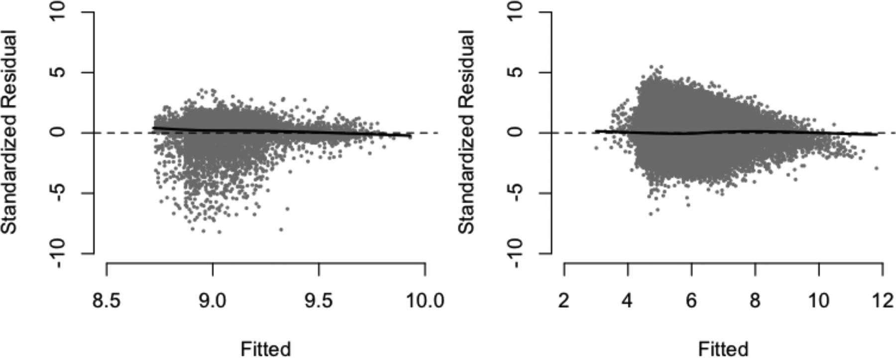
Fitted vs. (standardized) residual plots for the log-normal model for positive costs in the first interval (left) and follow-up intervals (right). LOESS smoothing curves are shown as black curves; the reference line (y = 0) is shown as a dashed line.
To further assess the ability of these models to perform adequately in the Monte-Carlo integration stage, we generated random draws from each of the two-part models at each covariate level in the data, and compared the distribution of the random draws to that of the true costs. In the original data, 2.27 % of the baseline costs and 25.6% of the non-baseline costs were zeros. From the generated predictions, the proportions were 2.37% and 25.6% respectively. Figure 5 depicts kernel density plots for the log non-zero costs at baseline and follow-up; these together illustrate that the cost-models used provide a reasonable fit to the data.
Figure 5:
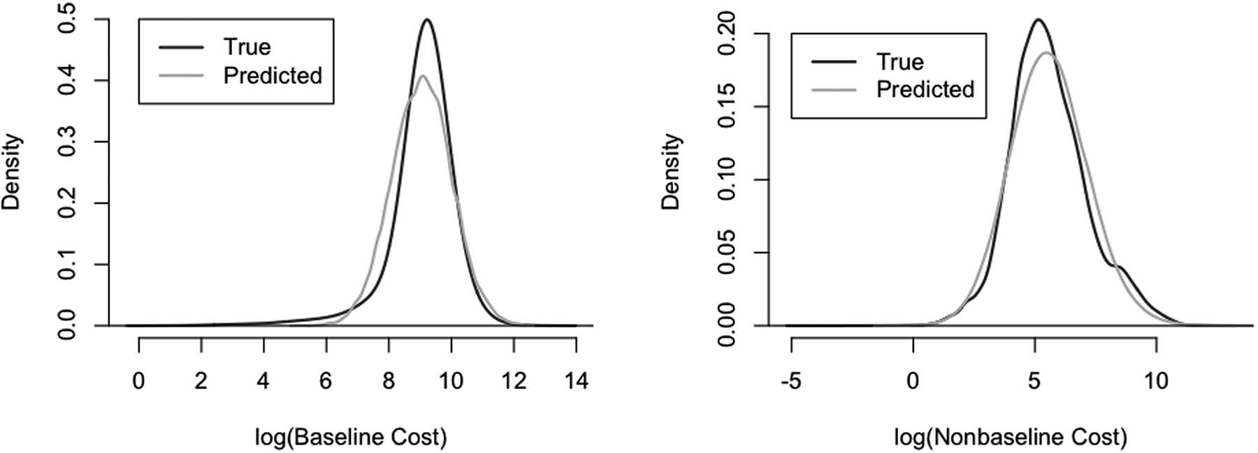
Kernel density plots of the predicted and true log-costs at baseline (left) and follow-up (right). The random draws generated appear to formulate a density that closely mirrors the empirical density from the data.
We consider five comparator post-surgery treatment regimes: (1) No treatment for all two years, (2) RT within the first month of surgery, (3) CT within the first month of surgery, (4) RT delayed for two months post-surgery, and (5) CT delayed for eight months post-surgery. These delays were chosen based on the median time-to-treatment among those ever receiving RT and CT, respectively. Table 5 depicts the estimated mean costs (in thousands of USD) under each of these treatment regimes, together with estimated standard errors and 95% Wald-based confidence intervals from the nonparametric bootstrap.
Table 5:
Results from an application to SEER-Medicare data. Depicted are the estimated costs (thousands of USD) under the five considered treatment regimes, along with the corresponding estimated bootstrap standard errors and 95% confidence intervals.
| Treatment | Est. | 95% CI | |
|---|---|---|---|
| None | 26.1 | 0.350 | [25.4, 26.8] |
| RT | 41.7 | 0.979 | [39.8, 43.6] |
| CT | 47.8 | 2.18 | [43.5, 52.1] |
| Delayed RT | 50.3 | 1.33 | [47.7, 52.9] |
| Delayed CT | 38.0 | 0.813 | [36.4, 39.6] |
Of note, the standard error considering CT immediately is markedly higher as compared to others; this is attributable to the fact that there are very few subjects receiving chemotherapy within the first month of hysterectomy. In general, these estimates are best suited for planning monetary resource allocation under a specific treatment regime. If, for instance, an eight-month delay in RT were chosen in an upcoming policy change, we estimate via nested g-computation that approximately $36.3k should be allocated per patient in this subpopulation. This insight could not have been gained with previously developed cost methods.
5.1. Sensitivity analysis
Identifying sufficiently many variables that predict the initial treatment assigment can be challenging in observational data. To address this, we now apply the sensitivity analysis procedure of Section 3.3 to evaluate the sensitivity of these results to departures from the assumption of ignorability of treatment assignment at baseline. We consider the setting of a single binary U with prevalence 0.5 (we could imagine this to be, for instance, a measure of functional status or an indicator of smoking history–which are not available in SEER-Medicare data). The sensitivity parameters are defined on a logit scale for the impact of U on treatment and probability of a zero cost, and on the linear scale for the log-transformed positive costs. We model the propensity of treatment on the logit scale, adjust for all confounders and include a natural cubic spline for age.
We consider three sets of sensitivity parameters to indicate varying levels of confounding; these coefficients were chosen to be, at maximum, only slightly more extreme than the model coefficients on the basis of the observed data. Table 6 summarizes the sensitivity parameters and their respective practical interpretations.
Table 6:
Characterization of sensitivity parameters under three scenarios (all are ratios that compare subgroups U = 1 to U = 0): γA (comparing odds of RT and/or CT), (compares odds of zero-cost), and (compares geometric mean cost in the first interval among those with nonzero cost).
| Scenario | Confounding level | γA | ||
|---|---|---|---|---|
| 1 | Low | 1.11 | 0.820 | 1.025 |
| 2 | Moderate | 1.28 | 0.719 | 1.105 |
| 3 | High | 1.65 | 0.613 | 1.220 |
Table 7 presents the results of this sensitivity analysis under the three established levels of confounding. As illustrated in Figure 6, the relative difference in estimated mean cost under each treatment regime under modest and moderate levels of confounding appear very comparable to those of the primary analysis; the relative pattern does not appear to hold as well under high levels of confounding. Importantly, we note similar ordering of costs across the treatment strategies are preserved. We conclude that our results were not sensitive to modest departures from the assumption of ignorability of baseline treatment assignment under the scenarios considered.
Table 7:
Results from a set of three sensitivity analyses for SEER-Medicare application. Depicted are the estimated costs (thousands of USD) under the five considered treatment regimes, along with 95% confidence intervals. Sensitivity analysis under different levels of confounding (modest, moderate, and high).
| Modest | Moderate | High | ||||
|---|---|---|---|---|---|---|
| Treatment | Est. | 95% CI | Est. | 95% CI | Est. | 95% CI |
| None | 23.3 | [22.8, 23.9] | 25.4 | [25.6, 27.1] | 29.9 | [29.2, 30.6] |
| RT | 33.6 | [32.3, 34.9] | 35.2 | [33.8, 36.6] | 38.9 | [37.3, 40.6] |
| CT | 38.5 | [35.3, 41.7] | 41.6 | [39.2, 42.5] | 40.9 | [37.5, 44.3] |
| Delayed RT | 39.2 | [37.5, 40.8] | 41.8 | [40.2, 43.5] | 47.6 | [45.5, 46.0] |
| Delayed CT | 34.6 | [33.1, 36.2] | 36.9 | [35.3, 38.5] | 41.6 | [39.9, 43.4] |
Figure 6:
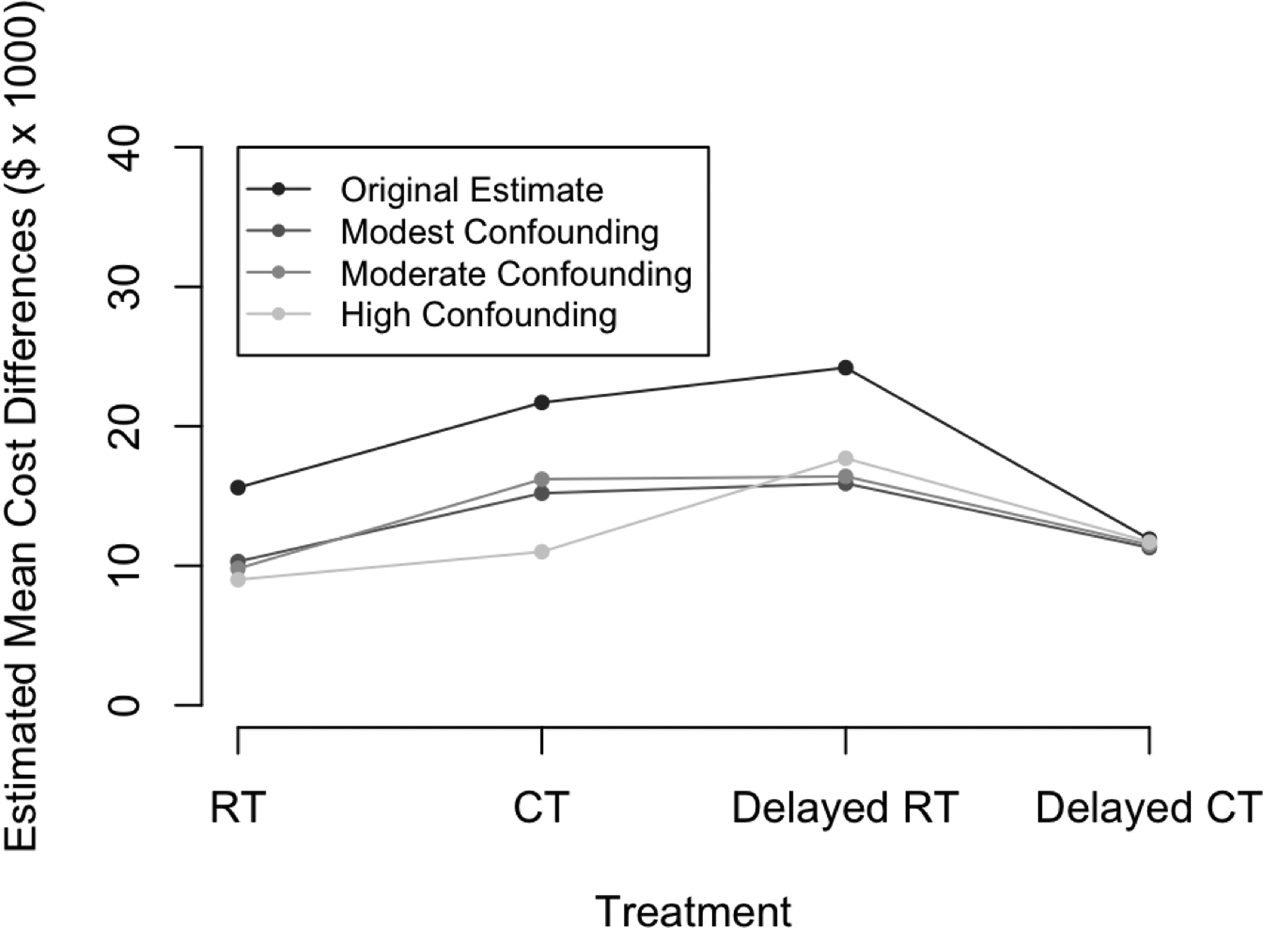
Illustration of the results of our sensitivity analysis. Depicted are the relative differences in estimated mean cost, considering each of RT, CT, delayed RT, and delayed CT relative to no treatment.
6. DISCUSSION
We have developed a nested g-computation framework to estimate marginal restricted-mean costs under user-specified treatment strategies. This approach, like previously explored inverse-probability weighting methods, addresses censoring, but has the advantage of allowing time-updating risk of death. Moreover, this approach targets a different parameter than those of existing approaches in that it provides a marginal mean under a joint treatment regime. The choice to target the marginal mean cost under an entire treatment strategy rather than the mean cost conditional on baseline treatment should be scientifically motivated. We argue that our approach is uniquely equipped to provide insights into issues surrounding monetary resource allocation, as explained in Section 5.
One priority of the Quality Payment Program is to develop alternate payment models for various health conditions such as cancer care. In designing these alternative payment models, physicians, payers, and policy makers are faced with a challenge of how to determine cost of care for a given treatment period or health-related condition. Historically, one might sum up approximate costs across all treatments incurred by a defined patient population over a set time period, though these methods would not account for changes in health over time, nor cumulative toxicities accrued during various treatments that may impact future care needs. Most methods have honed in on individual case costs and are not population-level in nature. The population-level estimands targeted by the nested g-formula are a sensible step towards appropriate allocation of resources and equitable reimbursements.
We caution, of course, against using this framework alone for direct comparison of costs in order to make treatment policy decisions, as it is possible that lower estimated costs could be the result of increased risks of death. Namely, without aggregating these data with insights into clinical effectiveness (the methodology of which is not the focus of this work), these data cannot be used to make recommendations regarding optimal treatment strategies. However, the purpose of this manuscript was to formalize a method to estimate the marginal mean costs, rather than to specifically compare those costs. Integrating this methodology into a cost-effectiveness framework is the subject of ongoing work, whereby treatment policy decisions could be made.
We have empirically demonstrated that the nested g-formula has favorable finite-sample properties including low bias, valid bootstrap standard errors, and proper coverage. Nonrandom subject dropout can be accommodated by the nested g-formula, at least to the extent to which the dropout is explainable by observable covariates. This gives the nested g-formula approach an advantage over alternative approaches that do not account for this commonly encountered limitation. In real-world data, zero costs can be common; moreover, the distribution of nonzero costs may be right-skewed, heteroscedastic, or heavier-tailed than assumed under the standard log-normal or Gamma models. The simulation results suggest that the nested g-formula is not overly sensitive to small discrepancies between the choice of methodology to account for right-skewness, nor overly sensitive to moderate amounts of unaddressed heteroscedasticity or heavy-tailedness in the data.
One potential limitation of this approach is the requirement for specification of several parametric models. This is quite important for cost outcomes that may, in practice, be substantially right skewed, or for which there may be a number of sampling zeros. Flexible modeling techniques such as two-part models and cubic splines can provide substantial improvements to model flexibility; on the other hand, Markov assumptions serve to reduce dimensionality and are one of the most effective ways to avoid over-fitting. Of note, justifications for invoking Markov assumptions should be specific to the problems to which they are being applied.
Further studies are warranted to better understand the scalability of this approach to high-dimensional covariates and many treatment times. Though a regularization approach could be used to improve mean-model flexibility, such approaches do not readily allow flexible sampling of the conditional error distribution, a necessary step in the nested g-computation procedure.
In observational databases, sensitivity analyses serve as a powerful tool that can help strengthen the validity of conclusions. The importance of sensitivity analyses in cost data has been previously discussed, and an approach was developed by Handorf et al. for the intent-to-treat methods (2013). We chose in our methodology to bypass the need to assume conditional independence of the unobserved and measured confounders, given treatment, due to the well-known phenomenon of collider bias that can result (Cole et al., 2009). In bypassing this problem, we are in exchange forced to model treatment propensities in the sensitivity analysis stage. Therefore, discrepancies between the results of a sensitivity analysis and the main analysis may be at least partly attributable to propensity score model misspecification. However, flexible modeling strategies can help curb this challenge; it is reassuring that (a) the ordering of the mean costs is preserved under the different levels of confounding, and (b) the costs under modest and moderate levels of confounding are very close to the estimated values in the main analysis. One could potentially approach the sensitivity analysis as a tipping-point analysis and determine the level of confounding that would be necessary to disturb the ordering of costs, for example. In order to accomplish this, one may need to specify differential effects of the unmeasured confounder on the different classes of treatment.
Principled approaches that aid us in giving insights into necessary levels of monetary resources are one of many reasonable steps toward responsible healthcare policies. Having access to information on hypothetical mean costs across entire treatment strategies can be immensely helpful for planning purposes to insurers, policy makers, and health economists, and can serve to efficiently and responsibly allocate monetary resources to particular patient subpopulations (women with Stage I and II endometrial cancer, in our motivating example). For the purposes of elucidating such marginal mean costs, we recommend use of the nested g-formula with flexible modeling approaches, together with sensitivity analyses under reasonable sets of sensitivity parameters.
Supplementary Material
Acknowledgements
This study was supported in part by NIH Grant R01 GM 112327 and Grant 124268-IRG-78-002-35-IRG from the American Cancer Society. This study used the linked SEER-Medicare database. The interpretation and reporting of these data are the sole responsibility of the authors. The authors acknowledge the efforts of the National Cancer Institute; the Office of Research, Development and Information, CMS; Information Management Services (IMS), Inc.; and the Surveillance, Epidemiology, and End Results (SEER) Program tumor registries in the creation of the SEER-Medicare database.
REFERENCES
- 1.American Cancer Society. Cancer Treatment & Survivorship Facts & Figures 2016–2017. Atlanta: American Cancer Society; 2016 [Google Scholar]
- 2.American Cancer Society. Facts & Figures 2018. American Cancer Society. Atlanta, GA; 2018. [Google Scholar]
- 3.Bang H and Tsiatis AA (2000), “Estimating medical costs from censored data,” Biometrika, 87(2):329–343. [Google Scholar]
- 4.Cole SR, Richardson DB, Chu H, and Naimi AI (2013), “Analysis of occupational asbestos exposure and lung cancer mortality using the g-formula,” American Journal of Epidemiology, 177(9):989–996. [DOI] [PMC free article] [PubMed] [Google Scholar]
- 5.Cole SR, Platt RW, Schisterman EF, Chu H, Westreich D, Richardson D, and Poole C (2009), “Illustrating bias due to conditioning on a collider,” International Journal of Epidemiology, 39(2):417–420. [DOI] [PMC free article] [PubMed] [Google Scholar]
- 6.Daniel R Cousens S, Stavola BD, Kenward M, and Sterne J (2013), “Methods for dealing with time-dependent confounding,” Statistics in Medicine, 32(9):1584–1618. [DOI] [PubMed] [Google Scholar]
- 7.Davison A and Hinkley D, Bootstrap Methods and their Application. Cambridge University Press, New York, 1997. [Google Scholar]
- 8.Dieleman JL, Squires E, Bui AL, Campbell M, Chapin A, Hamavid H, Horst C, Li Z, Matyasz T, Reynolds A, Sadat N, Schneider MT, Murray CJL (2017), “Factors associated with increases in US health care spending,” 1996–2013, The Journal of the American Medical Association, 318(17):1668–1678. [DOI] [PMC free article] [PubMed] [Google Scholar]
- 9.Handorf EA, Bekelman JE, Heitjan DF, and Mitra N (2013), “Evaluating costs with unmeasured confounding: A sensitivity analysis for the treatment effect,” The Annals of Applied Statistics, 7(4):2062–2080. [DOI] [PMC free article] [PubMed] [Google Scholar]
- 10.Herridge MS, Tansey CM, Matté A, Tomlinson G, Diaz-Granados N, Cooper A, Guest CB, Mazer CD, Mehta S, Stewart TE, Kudlow P, Cook D, Slutsky AS, and Chung AM (2011), “Functional disability 5 years after acute respiratory distress syndrome,” The New England Journal of Medicine, 364(14):1293–1304. [DOI] [PubMed] [Google Scholar]
- 11.H.R.2 - Medicare Access and CHIP Reauthorization Act of 2015. (2015). Available from: https://http://www.congress.gov/bill/114th-congress/house-bill/2/text.
- 12.Johnson BA and Tsiatis AA (2004), “Estimating mean response as a function of treatment duration in an observational study, where duration may be informatively censored,” Biometrics, 60(2):315–323. [DOI] [PubMed] [Google Scholar]
- 13.Johnson BA and Tsiatis AA (2005), “Semiparametric inference in observational duration-response studies, with duration possibly right-censored,” Biometrika, 92(3):605–618. [Google Scholar]
- 14.Li J, Handorf E, Bekelman J, and Mitra N (2016), “Propensity score and doubly robust methods for estimating the effect of treatment on censored cost,” Statistics in Medicine, 35(12):1985–1999. [DOI] [PMC free article] [PubMed] [Google Scholar]
- 15.Liao L, Jollis JG, Anstrom KJ, Whellan DJ, Kitzman DW, Aurigemma GP, Mark DB, Schulman KA, and Gottdiener JS (2006), “Costs for heart failure with normal vs reduced ejection fraction,” The Journal of the American Medical Association, 166(1):112–118. [DOI] [PubMed] [Google Scholar]
- 16.Lin D (2000), “Linear regression analysis of censored medical costs,” Biostatistics, 1(1):35–47. [DOI] [PubMed] [Google Scholar]
- 17.Lin D, (2003), “Regression analysis of incomplete medical cost data,” Statistics in Medicine, 22(7):1181–1200. [DOI] [PubMed] [Google Scholar]
- 18.Lin D, Feuer E, Etzioni R, and Wax Y (1997), “Estimating medical costs from incomplete follow-up data,” Biometrics, 53(2):419–434. [PubMed] [Google Scholar]
- 19.Lin D, Psaty B, and Kronmal R (1998), “Assessing the sensitivity of regression results to unmeasured confounders in observational studies,” Biometrics, 54(3):948–963. [PubMed] [Google Scholar]
- 20.Lu B (2005), “Propensity score matching with time-dependent covariates,” Biometrics. 61(3):721–728. [DOI] [PubMed] [Google Scholar]
- 21.Neugebauer R and van der Laan MJ (2006), “G-computation estimation for causal inference with complex logitudinal data,” Computational Statistics & Data Analysis, 51(3):1676–1697. [Google Scholar]
- 22.Papanicolas I, Woskie LR, and Jha AK (2018), “Health Care Spending in the United States and Other High-Income Countries,” The Journal of the American Medical Association, 319(10):1024–1039. [DOI] [PubMed] [Google Scholar]
- 23.Quality Payment Program (2017). Available from: https://qpp.cms.gov.
- 24.Robins J (1986), “A new approach to causal inference in mortality studies with a sustained exposure period–application to control of the healthy worker survivor effect,” Mathematical Modelling, 7(9–12):1393–1512. [Google Scholar]
- 25.Rubin D, (1978), “Bayesian inference for causal effects: the role of randomization,” The Annals of Statistics, 6(1):34–58. [Google Scholar]
- 26.Snowden JM, Rose S, and Mortimer KM (2011), “Implementation of g-computation on a simulated data set: Demonstration of a causal inference technique,” Americal Journal of Epidemiology, 173(7):731–738. [DOI] [PMC free article] [PubMed] [Google Scholar]
- 27.Spieker AJ, Roy JA, and Mitra N (2018), “Analyzing medical costs with time-dependent treatment: The nested g-formula,” To appear in Health Economics. [DOI] [PMC free article] [PubMed] [Google Scholar]
- 28.Taubman SL, Robins JM, Mittleman MA, and Hernán MA (2009), “Intervening on risk factors for coronary heart disease: an application of the parametric g-formula,” International Journal of Epidemiology, 28(6):1599–1611. [DOI] [PMC free article] [PubMed] [Google Scholar]
- 29.Westreich D, Cole SR, Young JG, Patella F, Tien PC, Kingsley K, Gange SJ, and Hernán MA (2012), “The parametric g-formula to estimate the effect of highly active antiretroviral therapy on incident AIDS or death,” Statistics in Medicine, 31(18):2000–2009. [DOI] [PMC free article] [PubMed] [Google Scholar]
- 30.Young JG, Cain LE, Robins JM, O’Reilly EJ, and Hernán MA (2011), “Comparative effectiveness of dynamic treatment regimes: an application of the parametric g-formula,” Statistics in Biosciences, 3(1):119. [DOI] [PMC free article] [PubMed] [Google Scholar]
Associated Data
This section collects any data citations, data availability statements, or supplementary materials included in this article.


