A practical guide to selecting models for exploration, inference, and prediction in ecology

Abstract

Selecting among competing statistical models is a core challenge in science. However, the many possible approaches and techniques for model selection, and the conflicting recommendations for their use, can be confusing. We contend that much confusion surrounding statistical model selection results from failing to first clearly specify the purpose of the analysis. We argue that there are three distinct goals for statistical modeling in ecology: data exploration, inference, and prediction. Once the modeling goal is clearly articulated, an appropriate model selection procedure is easier to identify. We review model selection approaches and highlight their strengths and weaknesses relative to each of the three modeling goals. We then present examples of modeling for exploration, inference, and prediction using a time series of butterfly population counts. These show how a model selection approach flows naturally from the modeling goal, leading to different models selected for different purposes, even with exactly the same data set. This review illustrates best practices for ecologists and should serve as a reminder that statistical recipes cannot substitute for critical thinking or for the use of independent data to test hypotheses and validate predictions.

Model selection is the Black Hole of Statistics.

A. Ronald Gallant, Liberal Arts Professor of Economics, Pennsylvania State University, and Henry A. Latane Distinguished Professor (emeritus) of Economics, UNC‐Chapel Hill (personal communication)

Introduction

In 2014, Ecology ran a productive and contentious Forum titled "P values, hypothesis testing, and model selection: it's déjà vu all over again" (Ellison et al. 2014). We learned a lot from the Forum—about common misunderstandings, the strengths and weaknesses of different approaches, and their underlying connections. But we still had no clear answer to many important questions. How should we decide among different approaches to model selection? When should we be doing model selection vs. using multi‐model inference (e.g., Burnham and Anderson 2002, Ver Hoef and Boveng 2015)?

We contend that model selection is essential in much of ecology because ecological systems are often too large and slow‐moving for our hypotheses to be tested through manipulative experiments at the relevant temporal and spatial scales. Because larch budmoth population cycles are a spatiotemporal process spanning all of western Europe (Bjornstad et al. 2002), an experiment to decisively test the hypothesis that the cycles are driven by parasitoids (Turchin et al. 2003) would have to eliminate those parasitoids from an entire continent while leaving all other factors undisturbed. To test the importance of dispersal for tropical forest species richness (Hubbell 2001, Volkov et al. 2003, 2005), we would need to block all seed dispersal onto Barro Colorado Island without affecting any other processes, and then wait many decades to observe the effect on canopy tree diversity. So instead, to identify the mechanisms underlying observed patterns and make predictions for planning and management, we often have to compare and choose among competing models fitted to imperfect observational data. Moreover, many manipulative experiments are designed to answer model‐selection questions: Are the data explained better by a model that includes the effect of particular covariates or their interactions? For example, is net primary production co‐limited by N and P (Fay et al. 2015)? Confusion about how to do model selection is confusion about how to do ecology.

Here we offer a guide to model selection based on the premise that carefully identifying the goal of an analysis—exploration, inference, or prediction—clarifies which model selection approaches should be used. A “best” model has to be best for some purpose, and different purposes will lead to different best models, even for the same data set. Much confusion has resulted from comparing and contrasting model selection methods without explicitly first asking: best model for what? Indeed, few books or papers in the ecology literature clearly specify the purpose of the model or acknowledge that different models should be selected for different goals (but see Shmueli 2010). This contrasts with the machine learning and statistical literature, where the modeling goal is often explicitly considered (e.g., Breiman 2001, Zou and Hastie 2005, Hastie et al. 2009, McElreath 2020). We are not the first to argue that model selection must be tailored to the purpose of the model (Rawlings et al. 1998), but we believe that the three goals listed above will be particularly useful for ecologists struggling with model selection.

To illustrate the problems and solutions, we focus on a common and challenging model selection problem in ecology: using observational data to link some time‐varying ecological response to interannual variation in weather. Populations, communities, and ecosystem‐level properties fluctuate through time in response to internal and external drivers. Internal drivers include intraspecific density dependence, demographic stochasticity, interspecific interactions, and food web dynamics. External drivers are typically related to environmental conditions, and weather is perhaps the most variable. Quantifying the relative impacts of internal forcing versus weather on ecological dynamics (Andrewartha and Birch 1954, Nicholson 1954) remains a core goal of ecology with new relevance as we attempt to predict ecological responses to climate change.

Unfortunately, detecting relationships between weather and ecological processes is surprisingly difficult. One issue is high dimensionality. Important ecological responses are often measured only one or two times a year (e.g., total aboveground biomass in permanent plots at the end of the growing season). But weather observations and gridded geospatial databases provide easy access to daily data on precipitation and mean, maximum, and minimum temperature, or some user‐defined summary of the series such as a frequency component (e.g., Elston et al. 2017). When these four variables are observed daily, we end up with 1,460 weather measurements over the course of a year. These covariates may be misaligned (Pacifici et al. 2019) or have compound effects over specific time periods. To link daily weather data to an annual ecological response in a statistical model, we must either aggregate the weather variables over some time period (van de Pol et al. 2016), or fit complex functional linear models to capture peaks of influence (Teller et al. 2016, Ferguson et al. 2017). In addition, the effects of some covariates may be nonlinear, making estimation and model selection even harder. So selection of weather covariates involves choosing (1) which weather variables to include (mean, maximum, or minimum temperature?), (2) the time periods when they matter (spring, summer, or both?), and (3) their functional form (linear, quadratic, logarithmic, etc.). The number of possible covariates can quickly grow much larger than the number of independent observations. To compound the difficulty, few ecological time series are long enough to offer the power to estimate more than a few covariate effects (Teller et al. 2016), temporal and spatial confounding may exist (Hodges and Reich 2010), and covariates may be collinear.

Because there are so many plausible weather covariates, the chance of finding spurious correlations is high. The temptation is to conduct an exploratory study and later portray it as a test of a priori hypotheses, hiding the multiple comparisons lurking below the surface of the analysis and undermining reproducibility. Linking weather to biological responses is therefore a classic model selection problem, representative of many in ecology and other disciplines. In fact, selecting among models that link weather to biological responses represents one of the worst‐case scenarios for model selection in ecology: statistical power is low because there are relatively few independent observations (Hodges and Reich 2010), the number of potential covariates is high, and a priori knowledge of what covariates to use may be limited.

Our focus on linking weather drivers to ecological dynamics is also motivated by our own failures. We have spent years trying to identify which weather covariates influence the population dynamics of perennial plant species in semiarid grasslands of the western United States. We have tried selecting among an a priori set of covariates via step‐wise model selection using both information‐theoretic criteria and P values (Dalgleish et al. 2011); we have tried detecting peaks of influence in time‐lagged weather covariates using functional linear models (Teller et al. 2016); and we have tried statistical regularization based on predicting out‐of‐sample data (Tredennick et al. 2017). At best, we have found statistically significant but weak absolute effects of weather, even though all our system‐specific knowledge tells us that in semiarid ecosystems plants should perform better when there is more water available. Even in cases where we did find statistically significant weather effects, they only marginally improved predictive skill (Tredennick et al. 2017, also see Matter and Roland 2017 for similar results). This paper is our attempt to make lemonade out of lemons. We want to share what we have learned from our struggles, and make model selection easier and more effective for others.

We focus primarily on covariate selection because it is a very common model‐selection problem in ecology, though it is certainly not the only model‐selection problem. Decisions about covariate transforms, model functional forms, and distributional assumptions all arise in the process of model checking, an essential part of any statistical analysis. The approach we advocate here should also provide guidance for these other aspects of model selection.

Model selection remains unsettled among statisticians

Ecology is not the only science struggling with model selection. In fact, it is an active area of research in statistics. Our perspective here follows well‐developed contemporary statistical frameworks, not only in ecology but across the sciences. In particular, we emphasize the need to separate null‐hypothesis significance testing from data exploration. This reflects the mathematical difficulty of describing how estimates and conclusions might vary across different data samples. Common statistical tests, applied to any one model, do not account for the fact that model selection violates assumptions on which the calculation and interpretation of P values depend.

One goal of contemporary statistical research is to develop methods for inference that account for model selection and associated uncertainty. Current approaches include selective inference (Taylor and Tibshirani 2015), stability selection (Meinshausen and Bühlmann 2010), and other methods (Shen et al. 2004, Lockhart et al. 2014, G'Sell et al. 2016). However, these methods only apply to particular models and applications (e.g., using LASSO to select covariates in a linear model). Bayesian statistics have a more solid theoretical foundation and methods like Bayesian model averaging offer formal ways to make inference that explicitly account for model selection and model selection uncertainty (Hoeting et al. 1999). However, there is currently no consensus in the statistics community about what constitutes correct practice, and there likely never will be. On the other hand, there is broad consensus on what constitutes poor practice, providing guidelines for model selection that we discuss here.

Many new approaches seek to extend the set of methods for which valid inference after model selection is possible, but they cannot solve the basic problem of researcher degrees of freedom: all of the implicit choices researchers make that influence an analysis (Simmons et al. 2011). For example, given a set of potential covariates and a chosen model‐selection method, it may be possible to obtain valid confidence intervals for the resulting coefficient estimates, but these will not account for choices such as data transforms, inclusion or not of interactions, or even the original choice of model‐selection method. It is always important to understand what actions in an inference procedure are accounted for in calculating uncertainty estimates such as P values or confidence intervals, and what constitutes data exploration beyond those boundaries.

Three Modeling Goals in Ecology: Exploration, Inference, and Prediction

We contend that ecologists fit statistical models for three primary purposes: data exploration, inference, and prediction. These goals are not mutually exclusive, though some combinations are forbidden or require independent studies (Fig. 1). In the following sections, we describe each goal and the model selection approaches most suited to each.

Fig. 1.

Venn diagram showing the (non)overlap of three modeling goals in ecology: data exploration, inference, and prediction or forecasting.

Exploration

The goal of exploration is to describe patterns in the data and generate hypotheses about nature. The textbook caricatures of the scientific method that emphasize the role of hypothesis testing are typically vague about where hypotheses come from. Some derive from theory, but often we arrive at them by induction from empirical patterns. The inductive approach is especially common in ecology, where many longstanding research topics involve identifying the processes driving canonical patterns such as the species‐area relationship or body size scaling relationships. The reliance on exploratory analyses may be especially pronounced in the search for relationships between weather and ecological processes, because we often lack a priori biological knowledge and want to consider many covariates (van de Pol et al. 2016).

The central trade‐off in exploratory modeling is the desire to be thorough vs. the need to avoid spurious relationships. To avoid missing potentially important relationships we should cast a wide net, considering all plausible associations. Modern statistical computing lets us examine hundreds of correlations or scatterplots with a few lines of code. It is also easy to fit large sets of nested models with different additive and multiplicative combinations of dozens of potential covariates, and compare them using some measure of model fit. But these approaches are prone to type‐I errors (false discoveries): in a data set with randomly generated “covariates,” we expect one in 20 correlations to be significant by chance at the α = 0.05 level. Generating hypotheses based on spurious correlations is a waste of time at best.

Fortunately, there are strategies that help strike a balance between thoroughness and avoiding false discoveries. Perhaps the most important, if obvious, strategy is to only consider plausible relationships, but the list of plausible relationships is often long. In such cases, methods to correct P values for multiple testing or multiple comparisons (such as p.adjust in R) can help reduce the chance of false discoveries. Finally, if we clearly communicate that our goal is exploration, meaning the generation but not the testing of hypotheses, the consequences of false discoveries are minimized. By assiduously avoiding any claims of confirmation, we can emphasize that the proposed hypotheses should not be accepted until they are tested with independent data.

Inference

The goal of modeling for inference is to evaluate the strength of evidence in a data set for some statement about nature. Gaining knowledge through inference requires alternative a priori hypotheses about how ecological systems function. These hypotheses are formalized as alternative statistical models that are confronted with data. Inference methods, such as null‐hypothesis significance tests, have been a primary focus of classical statistical theory. The fact that we need a priori models to represent each hypothesis puts a hard boundary between exploration and inference. We cannot formally test hypotheses on the same data set used to generate those hypotheses.

Inference does not require validation on independent data, because the goal is to determine whether or not a particular data set provides sufficiently strong evidence for a hypothesis. The risk of false discoveries due to over‐fitting is low because the distinguishing feature of studies aimed at inference is that contending a priori hypotheses are formalized as a small set of competing models, especially in the case of designed experiments. But what exactly is a “small set?” If the set includes just two models, we are clearly on safe ground for inference. Tests of some hypotheses may require three models. However, as the number of models grows, we should be increasingly skeptical about whether inference is truly the goal of the analysis, rather than exploration or prediction.

Statistical inference from a single data set is only one part of the process of developing scientific knowledge. It assesses the reliability of statements about a particular set of data obtained by particular methods under particular conditions. Any conclusions obtained via statistical inference thus require replication and validation across a range of conditions before they are accepted as scientific fact.

Prediction

Prediction is the most self‐explanatory modeling goal. Research aimed solely at prediction is relatively new in ecology, but calls for a formal research agenda centered on prediction and forecasting are accumulating (Clark et al. 2001, Petchey et al. 2015, Houlahan et al. 2016, Dietze et al. 2018, Harris et al. 2018). Modeling for prediction overlaps with modeling for exploration and inference because models that include our best understanding of a process should produce better forecasts (e.g., Hefley et al. 2017b ). For example, improved understanding can reduce the number of parameters in a model by replacing fitted coefficients with known values or swapping many potentially associated covariates for a few causal drivers. Moreover, confronting forecasts with new data is the ultimate test of our understanding (Houlahan et al. 2016, Dietze et al. 2018).

However, there is an important difference between modeling for inference and modeling for prediction, and recognizing this difference helps illuminate the model selection path. Consider a fitted regression model,

$$\widehat{\mathbf{y}}=\mathbf{X}\widehat{\mathrm{\beta }},$$ (1)

where X is the data matrix, $\widehat{\mathrm{\beta }}$ are the maximum likelihood estimates of the regression coefficients, and $\widehat{\mathbf{y}}$ is the predicted response.

Inference is about $\widehat{\mathrm{\beta }}$ (Gareth et al. 2017, Mullainathan and Spiess 2017). Which coefficients are non‐zero beyond a reasonable doubt, implying meaningful associations between covariates and the response? Which non‐zero effects are positive, and which are negative? Which covariates are more important and which are less important? The goal of modeling for inference is to answer these questions.

Prediction is about $\widehat{\mathbf{y}}$ (Gareth et al. 2017, Mullainathan and Spiess 2017). Which model will best predict values of y for new observations of the covariates in X?

Critically, the optimal model for prediction may not be suitable for inference. For example, extensive model selection to identify the optimal model for prediction complicates the interpretation of P values; regularization (see "Regularization" in next section) often improves prediction but biases parameter estimates; and machine learning methods may not provide interpretable coefficients. Furthermore, when many covariates are correlated, the optimal model for prediction is likely to include covariates having little actual association with the response (see Information‐theoretic approach ). Conversely, a model that provides reliable inference about the particular coefficients in β that represent a hypothesis of interest may not be optimal for prediction, if it excludes other relevant covariates. While understanding should generally improve predictions, discovering how to make the best predictions may not always improve understanding.

A distinguishing feature of modeling for prediction is the need to test predictive models “out of sample”: using independent data that were not used to fit the model. Exploratory modeling can help identify important predictors even if the causal mechanisms are currently not understood (Teller et al. 2016, van de Pol et al. 2016), but without validation on independent data, the predictive skill of the model is unknown.

Overview of Relevant Statistical Techniques

Before providing worked examples of modeling for exploration, inference, and prediction, we give brief descriptions of some statistical techniques we will use. We focus on frequentist methods. Proponents of a strict Bayesian framework might argue that separating the goals of exploration, inference, and prediction does not make sense. According to this view, testing out‐of‐sample performance falls outside Bayesian inference (Lindley 2000). However, most ecologists, and even many statisticians, apply Bayesian methods as a convenient alternative to fit a hierarchical model with MCMC methods, quantify uncertainty, accommodate nonlinear functions, or incorporate prior information on model parameters. For these practical applications of Bayesian methods, our advice will apply: identifying the purpose of the analysis remains a critical step in choosing a model selection strategy. We do, however, refer to the literature on Bayesian model selection methods (especially Hooten and Hobbs 2015) to show parallels between the frequentist methods we discuss and their Bayesian analogues.

Traditional null‐hypothesis significance testing

Traditional null‐hypothesis significance testing (NHST) compares a model of interest against a null model lacking some feature of the model of interest, such as a particular covariate. To compare models, we first need to calculate a summary of the data T, such as a z score or a t or F statistic. Model selection is based on the probability of observing a value of T more extreme than the value calculated from the data, if the model representing the null hypothesis is true. This probability is the P value; a small P value is interpreted as evidence for the model of interest.

Common statistical programs for ANOVA and regression by default report tests of a null hypothesis in which none of the independent variables affects the response variable. However, it is straightforward to work with more interesting null models. For example, if we want to test the hypothesis that winter snowpack negatively affects the population growth rate of an elk herd, the null model could include density dependence. We could then conduct a likelihood ratio test to ask if adding a snowpack covariate to this model significantly increases the likelihood of the data relative to the model with density dependence but not snowpack. The main limitation of the likelihood ratio test is that it can only be used for “nested” models, meaning that the covariates in the null model are also contained in the more complex model.

Bayes factors (Kass and Raftery 1995, Hooten and Hobbs 2015), a Bayesian analogue to likelihood ratios, are also used to compare competing statistical models. Unlike the likelihood ratio test, the competing models do not need to be nested. Bayes factors are often used like information criteria to rank models or to weight different models when model averaging (Link and Barker 2006).

Information‐theoretic approaches

Null‐hypothesis significance testing compares one model with another. In contrast, information‐theoretic approaches make it possible to compare the weight of evidence for any number of models. The most popular information‐theoretic criterion in ecology is Akaike's Information Criterion (AIC)

$$\text{AIC =}‐2\times \log \left[L\left(Y|\widehat{\mathrm{\theta }}\right)\right]+2p,$$ (2)

where $\widehat{\mathrm{\theta }}$ are the maximum likelihood estimates for model parameters and p is the number of parameters. Any number of models, nested or not, are easily ranked based on AIC values. Proponents of AIC argue that this approach avoids arbitrary P‐value cut‐offs (Burnham and Anderson 2002), but in practice researchers have relied on equally arbitrary and less interpretable cut‐offs for the difference in AIC values required to conclude that one model is more supported by the data than another.

It is important to recognize that AIC was created to advance the goal of prediction. Akaike's original purpose was to approximate a model's out‐of‐sample predictive skill, using only the data used to fit the model (Akaike 1973). This is a desirable feature for ecology, where data are hard‐won and we rarely have enough to set some aside for model validation. AIC approximates a model's out‐of‐sample skill by relying on an asymptotic approximation (Akaike 1973), so the estimate of information loss relative to the true data generating function becomes more unreliable as the size of the data set decreases. This also means that AIC provides relative, not absolute, measures of model predictive skill.

AIC is more forgiving of possibly spurious covariates than NHST, leading to models with more covariates, because of the asymmetry between the effect of omitting a relevant covariate and the effect of including a spurious one. Omitting a relevant covariate will limit a model's predictive skill, no matter how much data is available. However, if a spurious covariate is included, its impact on predictions will be very small when there are enough data to get good parameter estimates. This property of AIC makes it less suitable for inference than NHST. When circumstance requires its use for inference, for example to compare non‐nested models, results should be interpreted cautiously. The same is true for all model‐selection criteria based on prediction accuracy, including the cross‐validation methods discussed below. It is tempting to argue that the model making the best predictions must be closest to capturing the true mechanisms, but optimal models for prediction often include many potentially relevant but possibly spurious covariates, without giving any of them much weight in making projections.

There are several analogous Bayesian information criteria, including the deviance information criterion (DIC; Spiegelhalter et al. 2002), the Watanabe‐Akaike information criterion (WAIC; Watanabe 2013), and, most recently, approximate leave‐one‐out cross‐validation (LOO‐CV; Vehtari et al. [2017]). All have the same goal as AIC, using only within‐sample data to approximate the model's out‐of‐sample predictive accuracy. DIC is returned by common statistical packages, though WAIC and LOO‐CV are gaining popularity and are recommended in most cases (Gelman et al. 2014, Hooten and Hobbs 2015, Vehtari et al. 2017, McElreath 2020).

Regularization

Statistical regularization (Appendix S1: Section S2) refers to a suite of methods that seek to improve predictive accuracy by trading off between bias and variance in parameter estimates (Hastie et al. 2009). Regularization is relatively new to ecologists, even though AIC and related criteria are special cases (Hooten and Hobbs 2015). The term 2p in AIC (Eq. 2) regulates model complexity by penalizing the log‐likelihood based on the number of model parameters. Without this penalty, any comparison of nested models will result in the more complex model being chosen. This favors overly complex models that makes poor predictions on other data sets (Hastie et al. 2009).

More generally, regularization involves selecting a model or estimating parameter values based on a weighted average of a goodness‐of‐fit measure and a complexity penalty. For example, in penalized least‐squares regression, regression coefficients β are chosen to minimize

$$\sum _{i=1}^n{\left(y_i‐{\mathrm{\beta }}_0‐\sum _{j=1}^p{\mathrm{\beta }}_j{x}_{\mathit{ij}}\right)}^2+\mathrm{\gamma }r(\mathrm{\beta })$$ (3)

where r is a complexity penalty and the “regularization parameter” γ ≥ 0 determines the relative importance of the two terms. Common complexity penalties include ridge regression ($r={\sum }_{j=1}^p{\mathrm{\beta }}_j^2$) and LASSO ($r={\sum }_{j=1}^p\left|{\mathrm{\beta }}_j\right|$).

In standard least‐squares regression, coefficients are estimated with no penalty. To regularize the model, we re‐estimate the coefficients with increasing values of the regularization parameter, which results in shrinking the estimates towards zero. We then ask which regularization parameter value results in the best predictions for an independent data set.

A key feature of regularization is that coefficient or parameter values are moved away from the maximum likelihood or least‐squares estimates (Appendix S1: Fig. S1). Generally, this means the estimates are biased. This behavior must be considered when interpreting parameter estimates. Some penalty functions, such as LASSO, can shrink coefficients to exactly zero, thus performing automated variable selection. With others, such as ridge regression (Appendix S1: Section S2), coefficients may take very small values but do not go to zero.

Regularization in Bayesian methods is done by decreasing the prior variance of the regularized parameters (McElreath 2020). Examples in the ecological literature include Gerber et al. (2015) and Tredennick et al. (2017), among others. Indicator variable selection and Reversible‐jump MCMC are fully Bayesian, model‐based methods of model selection. We recommend Hooten and Hobbs (2015) for a review of these methods.

Model validation

When prediction is the goal, validation against out‐of‐sample data is imperative. This means comparing model predictions with observations that were not used to “train,” or fit, the model. Out‐of‐sample validation is important because it is easy for a model to reproduce patterns in the training data, but much harder to accurately predict the outcome in another situation, which is what we expect predictive models to do.

Out‐of‐sample validation (Appendix S1: Section S3) begins by randomly splitting the available data into training and validation sets. The randomization procedure should be stratified to account for temporal, spatial, or other structure in the data, otherwise predictive errors will be underestimated (Roberts et al. 2017). We then fit candidate models using the training data, use each model to make predictions for the validation data, and quantify model errors using a summary measure such as root mean squared error. The model with the lowest error is the best predictive model. Out‐of‐sample validation can be used to select among competing models, or to select the optimal penalty for a regularization method.

When data sets are too small for out‐of‐sample validation, we can use cross‐validation. In out‐of‐sample validation, the data set is split once and only once into training and validation sets. In cross‐validation the data set is split multiple times into training and validation sets. The data splits in cross‐validation are often referred to as folds: K‐fold cross‐validation means we do K different random splits. This leaves us with K out‐of‐sample error scores, which are averaged to obtain the cross‐validation score. In some cases, cross‐validation scores can be calculated or approximated without having to actually re‐fit the model multiple times (e.g., Hastie et al. 2009). Note that cross‐validation on small data sets is not free from problems: the effect of reducing sample size by removing observations can be substantial and the errors are correlated but not accounted for. Information criteria avoid these problems but come with their own set of limiting assumptions (see Regularization). We prefer cross‐validation because the problems are more transparent and the absolute scores are easier to interpret than the relative scores offered by information criteria.

Bayesian model validation is very similar to what we describe above. The functions used to quantify the difference between model predictions and observations may differ (e.g., posterior predictive loss is common for Bayesian models), but the approach is the same (Hooten and Hobbs 2015, McElreath 2020). We urge ecologists particularly interested in prediction and forecasting to investigate the importance of choosing appropriate model scores (Gneiting and Raftery 2007, Hooten and Hobbs 2015, Dietze et al. 2018).

Examples

Here, to illustrate how different modeling goals lead to different data analyses, we reanalyze one dataset as if we were writing three separate papers, each motivated by a different modeling goal. For each goal, we use a different subset of model and variable selection techniques introduced in the previous section, and we arrive at a different “best” model. We list sequential steps not to emphasize any specific statistical techniques, but rather to clearly outline the general approach. For example, we could have built a Prediction model using Random Forests instead of ridge regression; the important point is that for Prediction we optimize out‐of‐sample prediction accuracy, while for Inference we conduct an unbiased test of an a priori hypothesis.

The data are time series of population counts for subpopulations of an alpine butterfly, Parnassius smintheus (Roland and Matter 2016a , b ). Roland and colleagues have monitored the size of P. smintheus populations in 21 alpine meadows at Jumpingpound and Lusk Ridges, Alberta, Canada (50°57′ N, 114°54.3′ W) since 1995 (Roland and Matter 2016b ). They used mark–release–recapture methods to estimate population sizes (N_t) in each year (t) from 1995 to 2015, based on numbers of adults observed in August of each year. Using these population estimates, they calculated population growth rate from 1995 to 2014 as R_t = log₁₀(N_{t +1}/N_t), after adding 0.5 to all N_t before log‐transformation to account for zeros in the data. Roland and Matter provided these data along with over 90 potential weather covariates (Table 1 in Roland and Matter 2016b ). We restrict our analyses to 11 out of the 21 meadows that have observations in every year of the time series (Fig. 2).

Table 1.

Parameter estimates from the final model, with covariate selection done by dropping terms individually from the full model.

Covariate	Estimate	SE	t	drop1 P	Include	P (BH)	Include (BH)	P (Holm)	Include (Holm)
(Intercept)	−0.10	0.30	−0.33
decextmax	0.05	0.02	2.72	0.00	yes	0.00	yes	0.00	yes
decextmin	−0.02	0.00	−5.17	0.00	yes	0.00	yes	0.00	yes
logNt	−0.45	0.05	−8.30	0.00	yes	0.00	yes	0.00	yes
marmeanmax	−0.04	0.01	−2.46	0.01	yes	0.09	no	0.57	no
maymean	0.23	0.04	5.92	0.00	yes	0.00	yes	0.00	yes
novextmax	−0.07	0.01	−5.34	0.00	yes	0.00	yes	0.00	yes
novmeanmax	−0.03	0.02	−1.71	0.00	yes	0.00	yes	0.00	yes
octmeanmin	0.05	0.02	3.16	0.05	yes	0.56	no	1.00	no

The P values shown are from drop1.merMod applied to the full model with test = Chisq, not a t test. P(BH) and P(Holm) are the drop1 P values adjusted for multiple comparisons using the BH and Holm methods, respectively. decextmax: extreme maximum temperature in December; decextmin: extreme minimum temperature in December; logNt: (log) population size in the previous year; marmeanmax: mean maximum temperature in March; maymean: mean temperature in May; novextmax: extreme maximum temperature in November; novmeanmax: mean maximum temperature in November; octmeanmin: mean minimum temperature in October.

Fig. 2.

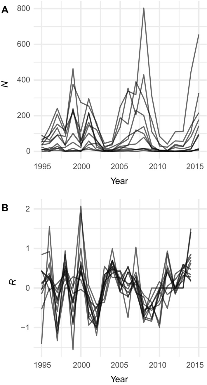
Time series of Parnassius smintheus butterfly abundance from Roland and Matter, (2016a ) for (A) raw population sizes and (B) log population growth rates. Each line is a subpopulation from one of 11 distinct meadows. N is population size; R is estimated population growth rate.

Roland and Matter's goal was to “identify specific weather variables that explain variation in population growth (R_t) from one summer to the next” (Roland and Matter 2016b :415), which sounds to us like modeling for exploration. However, they also sought to gain understanding because they wanted to confirm a previous, more general, finding that “winter weather” influenced P. smintheus population growth, a finding that is general across many butterfly species (Radchuk et al. 2013). Moreover, in a bold pair of papers, Matter and Roland first made explicit predictions of summer abundance in response to observed extreme winter weather (Matter and Roland 2015) and then discussed why those predictions were wrong, even though their models included statistically significant weather effects (Matter and Roland 2017). Matter and Roland have used these data for all three of our modeling goals, making this an ideal data set for demonstration. We bundled the data for our examples into an R package called modselr (see Data Availability). The analyses presented here can be reproduced using code in the archived version of this project's repository (se Data Availability).

Example: Exploration

Define the research question

If we lack a priori knowledge about the abiotic factors that regulate P. smintheus population dynamics, we can use statistical models to answer the question, “Which weather covariates are associated with population growth rates?” We will focus on selecting a model that best fits the entire data set, and we will consider an arbitrarily large set of candidate models, because we are not primarily concerned about the drawbacks of multiple comparisons. In a way, modeling for exploration is an “anything goes” exercise, so long as the results are clearly reported as a data exploration mission and the potential for spurious effects is carefully considered.

Screen many covariates for potential associations

Data visualization is a common way to perform an initial screening – in this case, we could plot population growth rate R_t against all available weather covariates, possibly adding a trend line. However, with 96 potential covariates this procedure seemed impractical and subjective. Instead, we proceeded in two stages: first, we calculated the correlation coefficient ρ between population growth rate and each covariate, and second, we plotted the fitted linear relationships for any response‐predictor relationship for which |ρ| > 0.3. The 15 relationships that cleared this bar all seem potentially important, and variation in the relationships among subpopulations appears small (Fig. 3).

Fig. 3.

Scatterplots of potential covariates vs. P. smintheus population growth rate (R_t). Covariates were screened before plotting, and only those with correlation higher than the arbitrarily chosen threshold (|ρ|>0.3) were plotted. Lines are fitted linear models for each subpopulation (meadow). Covariates are defined in Table 1 Notes.

Assess statistical evidence more rigorously

Our next step was to assess the statistical evidence for each of the 15 potentially important covariates' influence on the population growth rate. First, we fit a full model in a linear mixed‐effects framework, in which population growth rate was the response variable, the covariates shown in Fig. 3 were the fixed effects, and meadow (subpopulation) was a random effect on the intercept. Next, we used the stats::drop1() function to perform variable selection by comparing the full model to a series of reduced models in which one of the covariates was dropped. We fit all models using the R function lme4::lmer() (Bates et al. 2015). We then compared the full model to each of the reduced models using likelihood ratio tests. The results indicated that individually dropping seven of the 15 covariates did not significantly decrease the likelihood relative to the full model (they had P values > 0.05), so those should be removed from the model.

We fit a final model with the eight remaining covariates; coefficient estimates are shown in Table 1. The selected covariates suggest that temperatures in late fall, early winter, and spring affect population growth, consistent with analyses of the same data by Roland and Matter (2016b ). However, a close look at the estimates raises questions. Why would the effect of extreme maximum temperatures on population growth switch from negative in November (novextmax) to positive in December (decextmax), while minimum temperature effects switch from positive in October (octmeanmin) to negative in December (decextmin)? Similarly, why do March temperatures (marmeanmax) have negative effects on growth while May temperatures (maymean) have positive effects?

Correct for multiple comparisons

Since we started with 96 candidate covariates, we have reason to worry that some of these “significant” covariate effects might have appeared by chance. We applied two corrections for multiple comparisons to the drop1 P values from the full model, using p.adjust in base R, the Benjamini and Hochberg method (BH), which controls for the expected proportion of significant results that are spurious, and the Holm method (holm), which controls for the probability that one or more significant covariates is actually spurious. Both methods indicated that an additional two covariates should be dropped: March mean maximum and October mean minimum temperature (Table 1). Discarding those two effects helps resolve some of the apparent inconsistencies in the direction of effects. If we were writing these results up for publication, we would make it clear that, given the exploratory nature of our analysis and extensive model selection, the remaining covariates effects represent hypotheses that need to be tested using independent data.

Consider alternative approaches

The results from drop‐one model selection are conditional on the covariates we considered. We did not consider interactions among the covariates or covariates aggregated over different time periods, such as mean winter temperature over the months November to February. A useful technique when modeling for exploration is a sliding window analysis to compare models with different temporal aggregations of the covariates (van de Pol et al. 2016). The R package climwin is designed for that purpose.

We used the same linear mixed‐effects structure as in the drop‐one analysis, where population growth rate (R_t) is modeled as a function of some weather covariate and there is a random effect of meadow on the intercept. We looked only at mean monthly temperatures, but the analysis could easily be extended to identify the most influential climate window for any potential weather variables. We assumed that observations of population abundance occurred on 1 June of each year and we aggregated covariate values using the average over the specified window. Thus, a climate window that opens in month 4 (before the population observation) and closes in month 2 yields an aggregate covariate value that is the mean of the covariate over the February (month 4), March (month 3), and April (month 2) values.

The results identify December temperature as uniquely important, and the effect was positive (Fig. 4). Models focusing on March–May temperatures also receive some support (Fig. 4). Both of these findings are consistent with the results of analysis of single‐month covariates shown in Table 1.

Fig. 4.

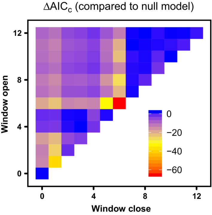
Sliding window analysis for mean temperature. The colors show the differences in AIC between a no‐climate null model and models fit to temperature averaged over windows that open and close a certain number of months before June, when populations are censused.

Example: Inference

Formulate competing hypotheses

Modeling for inference must begin with a priori hypotheses based on the literature or deduced from theory. For this example, we test the hypothesis that extreme high temperatures during early winter reduce P. smintheus population growth rate, but only in years of low snowfall (i.e., a temperature‐by‐snowfall interaction). The hypothesis comes from Roland and Matter (2016b ), which found evidence that butterfly eggs were vulnerable to extreme weather in early winter, especially in the absence of an insulating snowpack. This hypothesis does not address the potential role of spring weather identified in our exploratory analysis, because here we are starting over as if we had never conducted that analysis. We ask readers to temporarily ignore the fact that we are testing the hypothesis with the same data set used to generate it (Roland and Matter 2016b ), but we return to this key point below.

Translate hypotheses into alternative models

To test our hypothesis, we first created covariates that represent the key abiotic drivers. We defined early winter as November and December and then averaged two monthly covariates over that time: the maximum temperature and the amount of snow that fell each month. Note that we chose an arbitrary two‐month window for “early winter.” Other periods are probably equally defensible, but fitting multiple models with different winter covariates and selecting the “best” would weaken our inference.

We then specify the following model:

$$\mathbb{E}\left(x_{m,t+1}\right)={\mathrm{\beta }}_{0,m}+{\mathrm{\beta }}_{\text{dd}}{x}_{m,t}+{\mathrm{\beta }}_{\text{snow}}{x}_{\text{snow},t}+{\mathrm{\beta }}_{\text{temp}}{x}_{\text{temp},t}+{\mathrm{\beta }}_{\text{int}}\left(x_{\text{snow},t}\times x_{\text{temp},t}\right)+{\mathrm{\epsilon }}_{m,t}$$ (4)

where x_{m , t +1} is the log of population size in meadow m in year t + 1 x _snow is mean winter snow fall, x _temp is mean winter extreme maximum temperature, and ε_{m , t} are normally distributed residual errors. We included an interaction term (β_int) and accounted for variation among subpopulations by fitting a random intercept (β_{0, m}) for each subpopulation m. Last, we included the effect of current population size x_{m , t} to account for density dependence. We will compare this full model to an alternative null, or reduced, model that does not include the interaction effect.

Fit models

We fit the model in R using the lme4::lmer() function (Bates et al. 2015):

lmer(logNtnext ~ logNt + winter_mean_snow*winter_mean_extmax + (1|meada), data = test_data).

The estimated coefficients are shown in Appendix S1: Table S1.

Null‐hypothesis significance testing

To test the hypothesis that snow modifies the effect of winter temperature on P. smintheus population growth, we compared the full model described above with the alternative, reduced model that did not include the interaction effect. We performed a likelihood ratio test using the anova() function. The results show a significant interaction effect (χ² = 25.37, df = 1, P < 0.001), supporting the hypothesis. Rather than interpreting the effects directly from the coefficients, we generated a profile plot showing the marginal effect of maximum temperature on population size during low and high snow years, assuming mean population size. Fig. 5 shows a strong negative effect of temperature on population size in low snow years and no effect in high snow years. We did not test the significance of the individual main effects because our hypothesis focused on the snow × temperature interaction.

Fig. 5.

The model we built for inference shows an interactive effect of early winter maximum temperature and snow on Parnassius smintheus population size. The predicted growth rates shown here assume mean population size. Low snow corresponds to the 10% quantile for snow fall, and high snow corresponds to the 90% quantile.

The results would provide very strong confirmation of our hypothesis, except for the obvious problem: we did not test the hypothesis with independent data, we just re‐analyzed the data set used to propose the hypothesis (Roland and Matter 2016b ). Compounding the issue, the original analysis screened many covariates, increasing the potential for false discoveries. The solution would be to test the hypothesis with data collected from a different location or time period, or even from an experiment. Conversely, our analysis of the observational data would have been a strong test if the hypothesis had come from an independent source, such as laboratory studies of butterfly egg physiology.

Example: Prediction

Define the predictive goal

Our objective is to predict butterfly population size (on log scale) at time t given data on log population size in year t − 1 and information about weather during the period in between the observations.

Choose model selection approach

We chose regularization over AIC for two reasons. The first is convenience: whereas AIC would require us to specify and fit many different models with different sets of covariates, regularization offers a way to do variable selection in one step. Second, we did not want to rely on AIC's asymptotic approximation for predictive performance, when we can instead implement cross‐validation in our regularization approach.

Choose model validation approach

Although we used cross‐validation for model selection, we also wanted to validate the selected model against independent data. Therefore, we selected 19 of the 20 yr as a training data set, holding out the 20th year as a test, or validation, data set for quantification of predictive error.

Train the model

We used the glmnet package in R, which made it easy to compare the results from three different types of regularization: LASSO tends to produce a small number of strong effects, ridge regression produces many weak effects, and elastic net is a compromise between the two (Appendix S1: Section S2). In addition to weather covariates, which were penalized, all models included log population size the previous year, and separate intercepts for each meadow (implemented as fixed effects); none of these coefficients were penalized.

We used leave‐one‐year‐out cross‐validation within the training set to find the optimal value of the regularization parameter, γ, as follows. The procedure loops across all observation years in the training set, holding out a different year of data, k, on each pass through the loop. It then fits the regression model at a given γ value using the remaining years in the training set and makes out‐of‐sample predictions for the held‐out year k using the resulting coefficient estimates. This is repeated over an evenly spaced sequence of γ values from weak to strong. For each γ, the cross‐validation score is the mean squared error across the K cross‐validation folds (years), $(1/K){\sum }_{K=1}^K{(y_k^{\text{oos}}-{\widehat{y}}_k)}^2$ where $y_k^{\text{oos}}$ is an out‐of‐sample observation (other scores are possible, Hooten and Hobbs [2015]). γ was chosen to minimize the cross‐validation score. We then refit the model using the entire training set and the optimal γ, and used that model to predict population growth in each meadow in the test set year. The important point is that data from the test set were not used either to determine the optimal regularization parameter or to estimate coefficients. As a benchmark for the optimal regularized model, we fitted a null model without any climate covariates to the same training data set, and used it to generate a prediction for the validation set.

Test the model

With just one year in the validation set, a comparison of the prediction from the optimal regularized model and the null model has little power. If we had a longer time series, we could hold out more years for the validation set. Instead, we repeated the entire process outlined in the previous two steps 20 times, holding out one year for testing each time, and computed the mean squared prediction error for each hold‐out year.

We first tried including all 73 climate covariates that had no missing values, but found that the optimal regularized model made worse out‐of‐sample predictions than the null model. This was true whether we used LASSO, ridge regression, or elastic net. The lesson is that regularization and internal cross‐validation do not prevent over‐fitting when the number of covariates is so much greater than the number of independent observations.

Next, we used only the eight climate covariates identified by our Exploration analysis as potentially important. Using that subset of climate covariates in ridge regression, and considering all 20 of our independent validation tests, the optimal regularized model reduced mean squared error by roughly 15% relative to the null model (0.22 vs. 0.26; Fig. 6). A model that included all eight climate covariates and no regularization had larger estimated effects than the ridge regression model (Fig. 7B) and made worse predictions than the null model (MSE = 0.33). Thus, despite strong statistical evidence that winter weather influences butterfly population growth (Appendix S1: Table S1), the climate covariates had only modest value for prediction. Unfortunately, this seems to be a fairly common finding (Tredennick et al. 2017, Harris et al. 2018).

Fig. 6.

Comparison of out‐of‐sample predictions of butterfly population size, on the log scale, from a no‐climate null model and a ridge regression that included eight climate covariates. The black 1:1 line shows perfect agreement between observations and predictions. Different hold‐out years are shown by different color–symbol combinations. Mean squared errors were 0.26 for the null model and 0.22 for the ridge regression model.

Fig. 7.

(A) An example of how cross‐validated mean square error depends on the penalty term in the ridge regression, γ. For this example, data from 1995 were held out. (B) Regularization, implemented with ridge regression, shrinks the coefficient estimates toward zero relative to a model with the same climate covariates fit with no penalty.

After completing this analysis, we wondered if incorporating the process‐level understanding gained in our inference example might improve the predictions. We repeated the analysis after adding additional covariates to capture the early winter snow × temperature interaction. Mean squared error actually increased slightly relative to the model with the eight covariates reported in the preceding paragraph (not shown). Repeating the analysis using only the covariates featured in the inference example led to a much larger loss of predictive accuracy. These results are reminders that an understanding of process does not always translate directly into improved predictive skill.

For the butterfly data set, ridge regression performed better than LASSO or elastic net, indicating that population growth may be responding to many weak weather signals, rather than a few strong ones. Ridge regression tended to aggressively shrink even the largest coefficients (Fig. 7B), whereas LASSO shrunk weak effects to zero but did not shrink the strong effects as much.

Our demonstration analysis only produced point predictions. However, forecasting best practices call for quantitative estimates of uncertainty around predictions (Harris et al. 2018). We did not do this because there is currently no agreed‐upon method for calculating the uncertainty in predictions from a model obtained from LASSO‐type regularization, at least when using frequentist approaches. A Bayesian approach makes it easy to calculate uncertainty estimates, even with a regularized model, but caution is required in models with random effects. For example, hierarchical Bayesian models can absorb total uncertainty in the system in different components, making regularization difficult as one part of the system is squeezed and another part inflates. New statistical methods such as the “group LASSO” are emerging to tackle regularization of hierarchical models (Yuan and Lin 2006, Kyung et al. 2010, Hefley et al. 2017a ). For non‐hierarchical models, we urge those interested in making forecasts and quantifying uncertainty to seriously consider empirical Bayesian approaches to regularization, reviewed by Hooten and Hobbs (2015).

Guidance

Our focus on articulating the modeling goal prioritizes purpose over any particular statistical techniques for model selection. For each goal, various statistical techniques are appropriate, but not every statistical technique is appropriate for each goal (Table 2). For data exploration, almost any statistical tool can be justified. Some useful tools for model and variable selection are listed in Table 3. But an exhaustive search for statistical relationships should be balanced by an effort to focus on plausible relationships and findings should be communicated honestly, avoiding inferential claims. Corrections for multiple comparisons can help maintain this balance.

Table 2.

Model selection guidance.

Parameter	Exploration	Inference	Prediction
Purpose	generate hypotheses	test hypotheses	forecast the future accurately
Priority	thoroughness	avoid false positives	minimize error
A priori hypotheses	not necessary	essential	not necessary, but may inform model specification
Emphasis on model selection	important	minimal	important
Key statistical tools	any	null hypothesis significance tests	AIC; regularization; machine learning; cross‐validation; out‐of‐sample validation
Pitfalls	fooling yourself with over‐fitted models with spurious covariate effects	misrepresenting exploratory tests as tests of a priori hypotheses	failure to rigorously validate prediction accuracy with independent data

Table 3.

Some computing resources for model selection in R and Python.

Language	Package	Statistical techniques	Citation
R	glmnet	regularization via LASSO, ridge regression, and elastic net; cross‐validation	Friedman et al. (2010)
R	hiernet	LASSO regularization with hierarchy restrictions on inclusion of interaction terms	Bien et al. (2013)
R	glmmLASSO	LASSO for generalized linear mixed‐effects models	Grolls (2017)
R	climwin	moving window analysis for time‐indexed covariates	Bailey and van de Pol (2016)
R	loo	cross‐validation and model scoring with MCMC; stratified blocking for validation sets	Vehtari et al. (2020)
Python	scikit‐learn	machine learning; regularization via LASSO, ridge regression, and elastic net; cross‐validation	Pedregosa et al. (2011)

Modeling for inference requires a very small set of candidate models, directly linked to a priori hypotheses. If you have more than a handful of candidate models, it is likely that you are actually still in the exploration phase, or you may be more interested in prediction than inference. For inference, candidate models should ideally be evaluated with null‐hypotheses significance testing or by comparing Bayes factors. Information theoretic approaches can be used when candidate models are not nested, but with the caveat that tools like AIC are designed to approximate predictive performance, and may be less conservative than NHST about retaining additional covariates or other terms.

For prediction, the specific tool used for model selection is less important than the approach used to validate predictions. Quantifying predictive skill using independent data is essential. Predictive modeling often requires extensive model selection, for which information theoretic and regularization techniques are well‐suited.

The biggest danger is mixing modeling goals. It is often tempting to do inference after extensive model selection: taking reported P values from a final model at face value, even though the model was the result of extensive data exploration, or extensive model selection based on prediction accuracy (AIC or cross‐validation). In fact, many published studies pursue all three goals simultaneously. At least one of us has committed this sin more than once: Adler and Levine (2007) and Dalgleish et al. (2011) use long‐term observational data to study the effects of weather on species richness and plant vital rates, respectively. Both papers pursue fairly extensive variable selection, then draw inferences from the best models, and finally suggest that the results will improve predictions of ecological impacts of climate change. If we could write those papers over, we would either make the exploratory nature of the analyses much clearer, or we would cross‐validate to quantify predictive accuracy. We would certainly be far less casual about inference, because the parameter uncertainty resulting from extensive model selection is not accounted for in the P values from the final models.

Students may be discouraged by the message that rigorous generation and evaluation of hypotheses, or validation of predictive skill, often requires more than one data set. Fortunately, there are many creative ways to combine multiple data sets. Hypotheses generated from observational data sets can be tested with experiments (Adler et al. 2018) or vice versa, or predictions can be tested with data collected at new locations (Sequeira et al. 2016) or from different time periods (Veloz et al. 2012). Distributed experiments (Borer et al. 2014) offer additional opportunities: data from a subset of sites can be held out for hypothesis testing or model validation. Meta‐analysis is another approach for combining multiple data sets for the purpose of inference.

Our recommendations may also disappoint readers hoping for one‐size‐fits all solutions or simple statistical recipes. Each research problem and statistical analysis is unique, and shortcuts can never replace critical thinking. There are undoubtedly cases in which the best approach will be to ignore our advice! But we cannot imagine how time spent clearly articulating the purpose of the model could ever be time wasted.

Supporting information

Appendix S1

Tredennick, A. T. , Hooker G., Ellner S. P., and Adler P. B.. 2021. A practical guide to selecting models for exploration, inference, and prediction in ecology. Ecology 102(6):e03336. 10.1002/ecy.3336

Open Research

All data used in the manuscript is published on Dryad (Roland and Matter 2016a ) and has been bundled into an R data package (Tredennick 2020) available at https://doi.org/10.5281/zenodo.4311372. All computer code (Tredennick et al. 2020) is available at https://doi.org/10.5281/zenodo.4311358.

Literature Cited

- Adler, P. B. , Kleinhesselink A., Hooker G., Taylor J. B., Teller B., and Ellner S. P.. 2018. Weak interspecific interactions in a sagebrush steppe? Conflicting evidence from observations and experiments. Ecology 99:1621–1632. [DOI] [PubMed] [Google Scholar]
- Adler, P. B. , and Levine J. M.. 2007. Contrasting relationships between precipitation and species richness in space and time. Oikos 116:221–232. [Google Scholar]
- Akaike, H. 1973. Information theory and an extension of the maximum likelihood principle. Pages 267–281 in Petrov B. N. and Csaki F., editors. Proceedings of the 2nd International Symposium on Information Theory. Akadémiai Kiadó, Budapest, Hungary. [Google Scholar]
- Andrewartha, H. , and Birch L.. 1954. The distribution and abundance of species. Chicago University Press, Chicago, Illinois, USA. [Google Scholar]
- Bailey, L. D. , and van de Pol, M. 2016. climwin: An R Toolbox for Climate Window Analysis. PLoS ONE 11: e0167980. 10.1371/journal.pone.0167980 [DOI] [PMC free article] [PubMed] [Google Scholar]
- Bates, D. , Maechler M., Bolker B., and Walker S.. 2015. Fitting linear mixed‐effects models using lme4. Journal of Statistical Software 67:1–48. [Google Scholar]
- Bien, J. , Taylor J., and Tibshirani R.. 2013. A lasso for hierarchical interactions. Annals of Statistics 41:1111–1141. [DOI] [PMC free article] [PubMed] [Google Scholar]
- Bjornstad, O. , Peltonen M., Liebhold A., and Baltensweiler W.. 2002. Waves of larch budmoth outbreaks in the European Alps. Science 298:1020–1023. [DOI] [PubMed] [Google Scholar]
- Borer, E. T. , Harpole W. S., Adler P. B., Lind E. M., Orrock J. L., Seabloom E. W., and Smith M. D.. 2014. Finding generality in ecology: a model for globally distributed experiments. Methods in Ecology and Evolution 5:65–73. [Google Scholar]
- Breiman, L. 2001. Statistical modeling: The two cultures (with comments and a rejoinder by the author). Statistical Science 16:199–231. [Google Scholar]
- Burnham, K. P. , and Anderson D. R.. 2002. Model selection and multimodel inference. Springer, Berlin, Germany. [Google Scholar]
- Clark, J. S. , et al. 2001. Ecological forecasts: an emerging imperative. Science 293:657–660. [DOI] [PubMed] [Google Scholar]
- Dalgleish, H. J. , Koons D. N., Hooten M. B., Moffet C. A., and Adler P. B.. 2011. Climate influences the demography of three dominant sagebrush steppe plants. Ecology 92:75–85. [DOI] [PubMed] [Google Scholar]
- Dietze, M. C. , et al. 2018. Iterative near‐term ecological forecasting: Needs, opportunities, and challenges. Proceedings of the National Academy of Sciences USA 115:1424–1432. [DOI] [PMC free article] [PubMed] [Google Scholar]
- Ellison, A. M. , Gotelli N. J., Inouye B. D., and Strong D. R.. 2014. P values, hypothesis testing, and model selection: it’s déjà vu all over again. Ecology 95:609–610. [DOI] [PubMed] [Google Scholar]
- Elston, D. A. , et al. 2017. A new approach to modelling the relationship between annual population abundance indices and weather data. Journal of Agricultural, Biological and Environmental Statistics 22:427–445. [Google Scholar]
- Fay, P. A. , et al. 2015. Grassland productivity limited by multiple nutrients. Nature Plants 1:15080. [DOI] [PubMed] [Google Scholar]
- Ferguson, J. M. , Reichert B. E., Fletcher R. J. Jr., and Jager H. I.. 2017. Detecting population environmental interactions with mismatched time series data. Ecology 98:2813–2822. [DOI] [PMC free article] [PubMed] [Google Scholar]
- Friedman, J. , Hastie T., and Tibshirani R.. 2010. Regularization paths for generalized linear models via coordinate descent. Journal of Statistical Software 33:1–22. [PMC free article] [PubMed] [Google Scholar]
- G’Sell, M. G. , Wager S., Chouldechova A., and Tibshirani R.. 2016. Sequential selection procedures and false discovery rate control. Journal of the Royal Statistical Society: Series B (Statistical Methodology) 78:423–444. [Google Scholar]
- Gareth, J. , Witten D., Hastie T., and Tibshirani R.. 2017. An introduction to statistical learning with applications in R. Springer, New York, New York, USA. [Google Scholar]
- Gelman, A. , Hwang J., and Vehtari A.. 2014. Understanding predictive information criteria for Bayesian models. Statistics and Computing 24:997–1016. [Google Scholar]
- Gerber, B. B. D. , Kendall W. L., Hooten M. M. B., Dubovsky J. J. A., and Drewien R. C. R.. 2015. Optimal population prediction of sandhill crane recruitment based on climate‐mediated habitat limitations. Journal of Animal Ecology 84:1299–1310. [DOI] [PubMed] [Google Scholar]
- Gneiting, T. , and Raftery A. E.. 2007. Strictly proper scoring rules, prediction, and estimation. Journal of the American Statistical Association 102:359–378. [Google Scholar]
- Grolls, A. 2017. glmmLasso: Variable Selection for Generalized Linear Mixed Models by L1‐Penalized Estimation. R package version 1.5.1. https://CRAN.R‐project.org/package=glmmLasso
- Harris, D. J. , Taylor S. D., and White E. P.. 2018. Forecasting biodiversity in breeding birds using best practices. PeerJ 6:e4278. [DOI] [PMC free article] [PubMed] [Google Scholar]
- Hastie, T. , Tibshirani R., and Friedman J.. 2009. The elements of statistical learning: DataMining, inference, and prediction. Second edition. Springer, New York, New York, USA. [Google Scholar]
- Hefley, T. J. , Hooten M. B., Hanks E. M., Russell R. E., and Walsh D. P.. 2017a. The Bayesian group lasso for confounded spatial data. Journal of Agricultural, Biological and Environmental Statistics 22:42–59. [Google Scholar]
- Hefley, T. J. , Hooten M. B., Russell R. E., Walsh D. P., and Powell J. A.. 2017b. When mechanism matters: Bayesian forecasting using models of ecological diffusion. Ecology Letters 20:640–650. [DOI] [PubMed] [Google Scholar]
- Hodges, J. S. , and Reich B. J.. 2010. Adding spatially‐correlated errors can mess up the fixed effect you love. American Statistician 64:325–334. [Google Scholar]
- Hoeting, J. A. , Madigan D., Raftery A. E., and Volinsky C. T.. 1999. Bayesian model averaging: A tutorial. Statistical Science 14:382–401. [Google Scholar]
- Hooten, M. B. , and Hobbs N. T.. 2015. A guide to Bayesian model selection for ecologists. Ecological Monographs 85:3–28. [Google Scholar]
- Houlahan, J. E. , Mckinney S. T., Anderson T. M., and Mcgill B. J.. 2016. The priority of prediction in ecological understanding. Oikos 126:1–7. [Google Scholar]
- Hubbell, S. 2001. The unified neutral theory of biodiversity. Princeton University Press, Princeton, New Jersey, USA. [Google Scholar]
- Kass, R. E. , and Raftery A. E.. 1995. Bayes factors. Journal of the American Statistical Association 90:773–795. [Google Scholar]
- Kyung, M. , Gill J., Ghosh M., and Casella G.. 2010. Penalized regression, standard errors, and Bayesian lassos. Bayesian Analysis 5:369–411. [Google Scholar]
- Lindley, D. V. 2000. The philosophy of statistics. Journal of the Royal Statistical Society: Series D (The Statistician) 49:293–337. [Google Scholar]
- Link, W. A. , and Barker R. J.. 2006. Model weights and the foundations of multimodel inference. Ecology 87:2626–2635. [DOI] [PubMed] [Google Scholar]
- Lockhart, R. , Taylor J., Tibshirani R. J., and Tibshirani R.. 2014. A significance test for the lasso. Annals of statistics 42:413. [DOI] [PMC free article] [PubMed] [Google Scholar]
- Matter, S. F. , and Roland J.. 2015. A priori prediction of an extreme crash in 2015 for a population network of the alpine butterfly, Parnassius smintheus . Ecosphere 6:1–4. [Google Scholar]
- Matter, S. F. , and Roland J.. 2017. Climate and extreme weather independently affect population growth, but neither is a consistently good predictor. Ecosphere 8:e01816. [Google Scholar]
- McElreath, R. 2020. Statistical rethinking: A Bayesian course with examples in R and STAN. Chapman and Hall/CRC, New York, New York, USA. [Google Scholar]
- Meinshausen, N. , and Bühlmann P.. 2010. Stability selection. Journal of the Royal Statistical Society: Series B (Statistical Methodology) 72:417–473. [Google Scholar]
- Mullainathan, S. , and Spiess J.. 2017. Machine learning: An applied econometric approach. Journal of Economic Perspectives 31:87–106. [Google Scholar]
- Nicholson, A. J. 1954. An outline of the dynamics of animal populations. Australian Journal of Zoology 2:9–65. [Google Scholar]
- Pacifici, K. , Reich B. J., Miller D. A. W., and Pease B. S.. 2019. Resolving misaligned spatial data with integrated species distribution models. Ecology 100:e02709. [DOI] [PMC free article] [PubMed] [Google Scholar]
- Pedregosa, F. , et al. 2011. Scikit‐learn: Machine Learning in Python. Journal of Machine Learning Research 12:2825–2830. [Google Scholar]
- Petchey, O. L. , et al. 2015. The ecological forecast horizon, and examples of its uses and determinants. Ecology Letters 18:597–611. [DOI] [PMC free article] [PubMed] [Google Scholar]
- Radchuk, V. , Turlure C., and Schtickzelle N.. 2013. Each life stage matters: The importance of assessing the response to climate change over the complete life cycle in butterflies. Journal of Animal Ecology 82:275–285. [DOI] [PubMed] [Google Scholar]
- Rawlings, J. O. , Pantula S. G., and Dickey D. A.. 1998. Applied regression analysis: a research tool. Third edition. Springer Texts in Statistics, Springer New York, New York, New York, USA. [Google Scholar]
- Roberts, D. R. , et al. 2017. Cross‐validation strategies for data with temporal, spatial, hierarchical, or phylogenetic structure. Ecography 40:913–929. [Google Scholar]
- Roland, J. , and Matter S. F.. 2016a. Data from: Pivotal effect of early‐winter temperatures and snowfall on population growth of alpine Parnassius smintheus butterflies. Dryad, Dataset. 10.5061/dryad.tp324 [DOI]
- Roland, J. , and Matter S. F.. 2016b. Pivotal effect of early‐winter temperatures and snowfall on population growth of alpine Parnassius smintheus butterflies. Ecological Monographs 86:412–428. [Google Scholar]
- Sequeira, A. M. M. , Mellin C., Lozano‐Montes H. M., Vanderklift M. A., Babcock R. C., Haywood M. D. E., Meeuwig J. J., and Caley M. J.. 2016. Transferability of predictive models of coral reef fish species richness. Journal of Applied Ecology 53:64–72. [Google Scholar]
- Shen, X. , Huang H.‐C., and Ye J.. 2004. Inference after model selection. Journal of the American Statistical Association 99:751–762. [Google Scholar]
- Shmueli, G. 2010. To explain or to predict? Statistical Science 25:289–310. [Google Scholar]
- Simmons, J. P. , Nelson L. D., and Simonsohn U.. 2011. False‐positive psychology: Undisclosed flexibility in data collection and analysis allows presenting anything as significant. Psychological Science 22:1359–1366. [DOI] [PubMed] [Google Scholar]
- Spiegelhalter, D. J. , Best N. G., Carlin B. P., and Van Der Linde A.. 2002. Bayesian measures of model complexity and fit. Journal of the Royal Statistical Society. Series B: Statistical Methodology 64:583–639. [Google Scholar]
- Taylor, J. , and Tibshirani R. J.. 2015. Statistical learning and selective inference. Proceedings of the National Academy of Sciences USA 112:7629–7634. [DOI] [PMC free article] [PubMed] [Google Scholar]
- Teller, B. J. , Adler P. B., Edwards C. B., Hooker G., Snyder R. E., and Ellner S. P.. 2016. Linking demography with drivers: climate and competition. Methods in Ecology and Evolution 7:171–183. [Google Scholar]
- Tredennick, A. 2020. atredennick/modselr: v1.0 for ecology publication. Zenodo: https://zenodo.org/record/4311372
- Tredennick, A. , Hooker G., Ellner S., and Adler P.. 2020. A practical guide to selecting models for exploration, inference, and prediction in ecology. Zenodo. 10.5281/zenodo.4311358 [DOI] [PMC free article] [PubMed] [Google Scholar]
- Tredennick, A. T. , Hooten M. B., and Adler P. B.. 2017. Do we need demographic data to forecast plant population dynamics? Methods in Ecology and Evolution 8:541–551. [Google Scholar]
- Turchin, P. , Wood S., Ellner S., Kendall B., Murdoch W., Fischlin A., Casas J., McCauley E., and Briggs C.. 2003. Dynamical effects of plant quality and parasitism on population cycles of larch budmoth. Ecology 84:1207–1214. [Google Scholar]
- van de Pol, M. , Bailey L. D., McLean N., Rijsdijk L., Lawson C. R., and Brouwer L.. 2016. Identifying the best climatic predictors in ecology and evolution. Methods in Ecology and Evolution 7:1246–1257. [Google Scholar]
- Vehtari, A. , Gabry J., Magnusson M., Yao Y., Bürkner P., Paananen T., and Gelman A.. 2020. loo: Efficient leave‐one‐out cross‐validation and WAIC for Bayesian models. R package version 2.3.1. https://mc‐stan.org/loo
- Vehtari, A. , Gelman A., and Gabry J.. 2017. Practical bayesian model evaluation using leave‐one out cross‐validation and WAIC. Statistics and Computing 27:1413–1432. [Google Scholar]
- Veloz, S. D. , Williams J. W., Blois J. L., He F., Otto‐Bliesner B., and Liu Z.. 2012. No‐analog climates and shifting realized niches during the late quaternary: implications for 21st century predictions by species distribution models. Global Change Biology 18:1698–1713. [Google Scholar]
- Ver Hoef, J. M. , and Boveng P. L.. 2015. Iterating on a single model is a viable alternative to multimodel inference. Journal of Wildlife Management 79:719–729. [Google Scholar]
- Volkov, I. , Banavar J., He F., Hubbell S., and Maritan A.. 2005. Density dependence explains tree species abundance and diversity in tropical forests. Nature 438:658–661. [DOI] [PubMed] [Google Scholar]
- Volkov, I. , Banavar J., Hubbell S., and Maritan A.. 2003. Neutral theory and relative species abundance in ecology. Nature 424:1035–1037. [DOI] [PubMed] [Google Scholar]
- Watanabe, S. 2013. A widely applicable Bayesian information criterion. Journal of Machine Learning Research 14:867–897. [Google Scholar]
- Yuan, M. , and Lin Y.. 2006. Model selection and estimation in regression with grouped variables. Journal of the Royal Statistical Society: Series B (Statistical Methodology) 68:49–67. [Google Scholar]
- Zou, H. , and Hastie T.. 2005. Regularization and variable selection via the elastic net. Journal of the Royal Statistical Society Series B: Statistical Methodology 67:301–320. [Google Scholar]
Associated Data
This section collects any data citations, data availability statements, or supplementary materials included in this article.
Supplementary Materials
Appendix S1
Data Availability Statement