Chemically informed analyses of metabolomics mass spectrometry data with Qemistree

Abstract

Untargeted mass spectrometry is employed to detect small molecules in complex biospecimens, generating data that are difficult to interpret. We developed Qemistree, a data exploration strategy based on the hierarchical organization of molecular fingerprints predicted from fragmentation spectra. Qemistree allows mass spectrometry data to be represented in the context of sample metadata and chemical ontologies. By expressing molecular relationships as a tree, we can apply ecological tools that are designed to analyze and visualize the relatedness of DNA sequences to metabolomics data. Here we demonstrate the use of tree-guided data exploration tools to compare metabolomics samples across different experimental conditions such as chromatographic shifts. Additionally, we leverage a tree representation to visualize chemical diversity in a heterogeneous collection of samples. The Qemistree software pipeline is freely available to the microbiome and metabolomics communities in the form of a QIIME2 plugin, and a GNPS workflow.

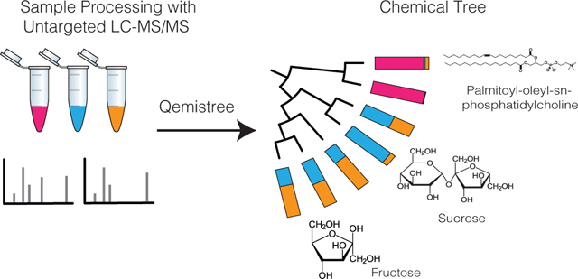
Graphical Abstract

Introduction

Molecular networking¹, introduced in 2012, was one of the first data organization approaches to visualize the relationships between tandem mass spectrometry (MS/MS) fragmentation spectra. In molecular networking, relationships between similar MS/MS spectra are visualized as edges. As MS/MS spectral similarity implies chemical structural similarity¹, chemical structural information can thus be represented as a network and chemical relationships can be visualized. This approach forms the basis for the web-based mass spectrometry infrastructure, Global Natural Products Social Molecular Networking² (GNPS, https://gnps.ucsd.edu/) which sees ~200,000 new accessions per month. Molecular networking has successfully been used for a range of applications³ in drug discovery, natural products research, environmental monitoring, medicine, and agriculture. To tap into the chemistry of complex samples through metabolomics, a subset of MS/MS spectra can be annotated by spectral library matching or by using in silico approaches. While molecular networking facilitates the visualization of closely related molecules in molecular families, the inference of chemical relationships at a dataset-wide level and in the context of diverse sample metadata requires complementary representation strategies. To address this need, we developed an approach that uses fragmentation trees⁴ and machine learning⁵ to calculate all pairwise chemical relationships. These chemical relationships are represented as a chemical tree that can be visualized in the context of sample metadata and molecular annotations obtained from spectral matching and in silico annotation tools. We show that such a chemical tree representation enables the application of various tree-based tools, originally developed for analyzing DNA sequencing data^6–9, for exploring mass-spectrometry data.

Here, we introduce Qemistree (pronounced chemis-tree) software that constructs a chemical tree based on predicted molecular fingerprints from MS/MS fragmentation spectra¹⁰. Molecular fingerprints are vectors where each position encodes a substructural property of the molecule, and recent methods allow us to predict molecular fingerprints from tandem mass spectra^11–15. In Qemistree, we use SIRIUS¹⁶ and CSI:FingerID¹³ to obtain predicted molecular fingerprints. Users can first perform feature detection^17,18 to generate a list of observed ions with associated peak areas and MS/MS fragmentation spectra, referred to as chemical features henceforth, to be analyzed by Qemistree (Extended Data Fig. 1). Only chemical features with MS/MS data are included; features with only MS1 are not considered. SIRIUS then determines the molecular formula of each feature using the isotope and fragmentation patterns and estimates the best fragmentation tree explaining the fragmentation spectrum. Subsequently, CSI:FingerID operates on the fragmentation trees using kernel support vector machines to predict molecular properties (2936 properties; Supplementary Dataset 1). We use these molecular fingerprints to calculate pairwise distances between chemical features and hierarchically cluster the fingerprint vectors to generate a tree representing their chemical structural relationships. Although alternative approaches to hierarchically cluster features based on cosine similarity of fragmentation spectra exist^19–21, we use molecular fingerprints predicted by CSI:FingerID for this. Previous work has shown that CSI:FingerID outperforms other tools for automatic in silico structural annotation²². Therefore, we leverage it to search molecular structural databases to provide complementary insights into structures when no match is obtained against spectral libraries. Subsequently, we use ClassyFire²³ to assign a 5-level chemical taxonomy (chemical kingdom, superclass, class, subclass, and direct parent ontology) to all molecules annotated via spectral library matching and in silico prediction (Supplementary Tables 1 and 2 include an assessment of improved annotation rates).

Phylogenetic tools such as iTOL²⁴ can be used to visualize Qemistree trees interactively in the context of sample information and feature annotations for easy data exploration. The outputs of Qemistree can also be plugged into other workflows in QIIME 2 (ref. ²⁵; many of which were originally developed for microbiome sequence analysis) or in R, Python, etc. for system-wide metabolomic data analyses ^{6,7,9, 26}. In this study, we apply Qemistree to perform chemically informed comparisons of samples in the presence of technical variation such as chromatographic shifts that commonly affect mass spectrometry data analysis. Additionally, we exemplify the use of a tree-based representation to visualize and explore chemical diversity using a heterogeneous collection of food products. Qemistree can be used iteratively to incorporate multiple datasets without the need for cumbersome reprocessing (such as repeated feature detection or retention time alignment), allowing for large-scale dataset comparisons. Qemistree is available to the microbiome community as a QIIME 2 plugin (https://github.com/biocore/q2-qemistree) and the metabolomics community as a workflow on GNPS² (https://ccms-ucsd.github.io/GNPSDocumentation/qemistree/). The chemical tree from the GNPS workflow can be explored interactively using the Qemistree-GNPS dashboard. (https://qemistree.ucsd.edu/; see Online Methods).

Results

Resolving technical variation using chemical relationships

To verify that molecular fingerprint-based trees correctly capture the chemical relationships between molecules, we designed an evaluation dataset using four distinct biological specimens: two human fecal samples, a tomato seedling sample, and a human serum sample. Samples were prepared by combining them in binary, tertiary, and quaternary mixtures in various proportions to generate a set of diverse but related metabolite profiles (Supplementary Table 3). Untargeted tandem mass spectrometry was used to analyze the chemical composition of these samples and obtain fragmentation spectra. The mass spectrometry experiments were performed twice using different chromatographic elution gradients, causing a retention time shift between the two runs (Extended Data Figs. 2 and 3). Processing the data of these two experiments with traditional LC-MS-based pipelines leads to the same molecules being detected as different chemical features in downstream analysis. Figure 1 shows the analysis of pure samples to demonstrate this. In Extended Data Figure 4, we highlight how these technical variations make the same samples appear chemically disjointed.

Figure 1: Qemistree mitigates aspects of technical artifacts by co-clustering structurally similar molecules across mass spectrometry runs.

A chemical tree based on predicted molecular fingerprints representing the structural relationships between compounds detected in the evaluation dataset. The outer ring shows the relative prevalence of molecules stratified by mass spectrometry run; the inner ring shows the same stratified by fecal, serum and tomato samples in the evaluation dataset. All structures shown are spectral reference library matches obtained from feature-based molecular networking^17,18 in GNPS (level 2 or 3 according to the 2007 Metabolomics Standards Initiative²⁷). Note that untargeted mass spectrometry is blind to stereochemistry and often regiochemistry (e.g. double bonds in a fatty acid), therefore molecules could be related isomers of the illustrated structures.

Using Qemistree, we mapped each of the spectra in the two chromatographic conditions (batches) to a molecular fingerprint, and organized these in a tree structure (Figure 1). Because molecular fingerprints are independent of retention time shifts, spectra are clustered based on their chemical similarity. It is noteworthy that the structural information from chemical features with spectral library matches (typically 1–20% of all features, depending on how well the sample type has been investigated) or other forms of annotation (e.g. substructure Mass2Motifs²⁸) could also be used to compare the chemical composition of samples across different mass spectrometry runs. Qemistree improves upon this by enabling the use of all MS/MS spectra with molecular fingerprints (86.90% in these data at the present time; Supplementary Table 1) for downstream comparative analyses, by not constraining analysis to the chemical features with spectral matches only. This tree structure can be decorated using sample type descriptions, chromatographic conditions, spectral matches obtained from molecular networking in GNPS (when available), and any other chemical annotations^23,28. Figure 1 shows that similar chemical features were detected exclusively in one of the two batches. However, based on the molecular fingerprints, these chemical features were arranged as neighboring tips in the tree regardless of the retention time shifts. This result shows how Qemistree can reconcile and facilitate the comparison of datasets acquired on different chromatographic gradients.

Tree-guided system-wide comparisons in metabolomics

Having demonstrated Qemistree’s practical utility on biologically inspired synthetic datasets, we now turned to a conceptual example illustrating the general principle. We demonstrated an application of a chemical hierarchy in performing chemically informed comparisons of metabolomics profiles. In standard metabolomic statistical analyses, each molecule is assumed unrelated to the other molecules in the dataset. Some of the pitfalls of this assumption are highlighted in Figure 2a. Consider a scenario where we want to compare samples 1–3. An analysis schema that does not account for the chemical relationships among the molecules in these samples (Figure 2a, left), will assume that the sugars in samples 2 and 3 are as chemically related to the lipids in sample 1 as they are to each other. This would lead to the naive conclusion that samples 1 and 2, and samples 2 and 3 are equally distinct, yet from a chemical perspective they are not. On the other hand, if we account for the fact that sugar molecules are more chemically related to one another than they are to lipids, we can obtain a chemically informed sample-to-sample comparison.

Figure 2: The pitfalls of assuming equal relatedness of molecules and the advantages of a chemical tree for sample comparison.

a) A scenario where the goal is to compare the chemical composition in three samples, and the consequences of accounting for or ignoring molecular relatedness. b, c) PCoA of all samples (N=162) in the evaluation dataset colored by chromatography conditions. PCoA plot using tree-agnostic (Bray-Curtis³⁰) distances which do not account for the chemical relationship between features detected across chromatography conditions (b) and tree-based (Weighted UniFrac⁹) distances which are based on the hierarchical relationships between molecules in the evaluation dataset (c).

The chemical structural compositional similarity (CSCS) metric²⁹ was developed to compute pairwise sample-to-sample comparison by considering cosine similarity of MS/MS spectra from molecular networking. Here, we utilize a tree-based approach to account for chemical relationships, which allows us to adopt phylogeny-based tools for metabolomics analyses (Supplementary Table 4). Specifically, we first constructed a tree of chemical similarities by hierarchical clustering molecular fingerprints from CSI:FingerID (using pairwise Euclidean distance between fingerprint vectors; see Online Methods). This tree is analogous to phylogenetic trees used in ecology, such that the tips of the tree are molecules (instead of species). We then computed weighted UniFrac⁹ distances (a tree-based metric that has widely been used in microbial ecology to compare microbiomes) to compare metabolomic profiles. In Figure 2a, we show that by using a tree of chemical relationships between molecules in samples 1–3, we can visualize that sample 1 is chemically very distinct (along PC1) from samples 2 and 3.

Returning to our evaluation dataset, we can highlight the importance of comparing samples by accounting for their molecular relatedness. Principal coordinates analysis (PCoA) of the evaluation dataset (including both pure samples and sample mixtures, N=162) that ignores the tree structure (Fig. 2b) performs far worse than the Qemistree PCoA that uses the tree (Fig. 2c). With the structural context provided by Qemistree, the differences between replicates across batches are comparable to the within-batch differences (Extended Data Fig. 5). The retention time shift in this dataset leads to a strong signal due to chromatography conditions that obscures the biological relationships among the samples (permutational ANOVA; tree agnostic³⁰ pseudo-F=120.75, p=0.001 vs. tree informed⁹ pseudo-F=18.2239, p=0.001). We observed and remediated a similar pattern originating from plate-to-plate variation in a recently published study investigating the metabolome and microbiome of captive cheetahs³¹ (Extended Data Fig. 6). In this study, placing the molecules in a tree using Qemistree reduced the observed technical variation (Extended Data Fig. 6a,c), and highlighted the dietary effect that was expected (Extended Data Fig. 6b,d). These results show how systematic and spurious molecular differences can be mitigated in an unsupervised manner using chemically informed distance measures based on a tree structure.

Visualizing chemical prevalence in heterogeneous datasets

As a case study demonstrating the utility of Qemistree on a set of biological specimens, we used the platform to explore chemical diversity in food samples collected in the Global FoodOmics initiative (http://globalfoodomics.org). Understanding the chemical relationships between different foods is challenging because most molecules within foods are unannotated. We selected a diverse range of food ingredients to represent animal, plant, and fungal groupings³². We first performed feature-based molecular networking using MZmine^17,18 to obtain spectral library matches for a subset of the chemical features (~20% annotated with cosine cutoff > 0.7). Using Qemistree, we collated GNPS spectral library matches and in silico predictions from CSI:FingerID to annotate ~91% of the chemical fingerprints (total 663 after quality filtering; Supplementary Table 1) with molecular structures. We also retrieved chemical taxonomy assignments for structures that were classified by ClassyFire²³ (~ 92% of all structures at the time of submission); the remaining are in the queue to be processed on the ClassyFire server for taxonomy assignment (see Online Methods). Labeling annotations allowed us to retrieve subtrees of distinct chemical classes (Fig. 3a) such as flavonoids, alkaloids, phospholipids, acyl-carnitines, and O-glycosyl compounds in food products. We propagated ClassyFire annotations of chemical features (tree tips) to each internal node of the tree and labeled the nodes by pie charts depicting the distribution in chemical superclasses (Extended Data Fig. 7) and classes (Extended Data Fig. 8) of its tips. The molecular fingerprint-based hierarchy of chemical features agreed well with ClassyFire taxonomy assignment, further demonstrating that molecular fingerprints can meaningfully capture structural relationships among molecules in a hierarchical manner. Furthermore, Qemistree coupled the chemical tree to sample metadata, revealing distinct chemical classes expected for each sample type. Branches representing acyl-carnitines were exclusively found in animal products (Fig. 3a). In contrast, honey, although categorized as an animal product, shared most of its chemical space with plant products, reflective of the plant nectar and pollen-based diet of honey bees. We observed a clade of flavonoids in both plant products and honey (Fig. 3, Extended Data Fig. 8), but no other animal-based foods.

Figure 3: A chemical hierarchy of food-derived compounds based on predicted molecular fingerprints.

A chemical tree based on molecular fingerprints representing the structural relationships between chemical features (tree tips) detected in food products (single ingredient i.e. simple foods; N=119). The tree is pruned to only keep tips that were assigned a structural annotation (SMILES) by either MS/MS spectral library matching or in silico using CSI:FingerID. All structures shown are spectral reference library matches obtained from feature-based molecular networking in GNPS). The outer ring shows the relative abundance of each compound across a diverse range of food sources. We highlight clusters of compounds that are characteristic of specific food sources.

While it is expected that a complex food such as blueberry kefir contains molecules from both blueberries and dairy, we can now visualize how individual ingredients and food preparation contribute to the chemical composition of complex foods. We noted that metabolite signatures that stem directly from particular ingredients, such as phosphoethanolamine from eggs, are present in egg scramble (Fig. 4b), but not in the other two foods highlighted (Fig. 4a,c). We can also observe the addition of ingredients in foods that were not listed as present in the initial set of ingredients. We were able to retrieve that there is black pepper in the egg scramble with chorizo and orange chicken, but that this signal is absent from the blueberry kefir (Extended Data Fig. 9).

Figure 4: A hierarchy of the compounds observed in simple foods and seven complex samples.

(a–c) Hierarchies of the compounds observed in simple foods and seven complex samples: two meals of orange chicken, a cooked cucumber and the sauce from a meal (schmorgurken), sour cream, blueberry kefir, and egg scramble with chorizo (N=126 samples). Top, the inner rings show the relative abundance of each compound across simple animal products, plant products, fungi and algae (other) and the seven complex foods (black). In the outer rings, the absolute abundances of compounds in blueberry kefir (a), scrambled eggs with chorizo (b), and orange chicken (c) are overlaid on the trees to illustrate the shared and unique chemistry of complex foods. Below, compound subtrees for representative compounds from each meal are highlighted. Note that untargeted mass-spectrometry is blind to stereochemistry and oftentimes regiochemistry (e.g. double bonds in a fatty acid); the structures shown are based on the spectral annotation of the reference library. This equals level 2 or 3 according to the 2007 metabolomics standards initiative²⁷.

Discussion

We show that our tree-based approach coherently captures chemical ontologies and relationships among molecules and samples in various publicly available datasets. Qemistree depends on representing chemical features as molecular fingerprints, and does share limitations with the underlying fingerprint prediction tool CSI:FingerID. For example, fingerprint prediction depends on the quality and coverage of MS/MS spectral databases available for training the predictive models, and these will improve as databases are enriched with more compound classes. Nevertheless, the use of CSI:FingerID-predicted molecular fingerprints is highly advantageous. While annotations from spectral matches may be more accurate, their coverage is too low to adequately summarize the chemical content of complex samples. Qemistree is also applicable in negative ionization mode; however, fewer molecular fingerprints can be confidently predicted due to fewer publicly available reference spectra, resulting in less-extensive trees.

A key contribution of this work is to introduce the concept of building chemical hierarchies that can be used to leverage phylogeny-based tools (which have been highly advantageous for DNA sequencing analysis), for metabolomics data exploration. Hierarchical relationships have provided a powerful framework to understand the relatedness of organisms. These techniques form a cornerstone for the interpretation of genomics data with phylogenetics and phylogenomics, and even taxonomy. The suite of tools and algorithms that have been developed over the past few decades in these fields, which utilize hierarchical structures, potentially have general relevance to the investigation of mass spectrometry data. Using Qemistree we can begin to explore the applicability of other methods, such as Faith’s Phylogenetic Diversity⁷ to understand within-sample complexity, or phylogenetic-independent contrasts³³ with a metabolomics-inspired topology as these representations enter regular use.

We showed that a hierarchical representation could be used to infer chemically informed relationships between samples (Fig. 2). While we used molecular fingerprints predicted by CSI:FingerID to build chemical hierarchies here, this approach can be extended to incorporate other strategies to compare molecules for building chemical trees. For example, chemical relationships based on assigned chemical classes²³, spectral motifs²⁸, shared biosynthetic origin³⁴ or other structural comparison methods³⁵ could also be used as a basis for such a tree. These approaches will result in different tree topologies capturing complementary chemical information for subsequent analyses. Ultimately, a broader benchmarking effort would be needed to understand when each approach should be used, similar to benchmarking efforts in the environmental DNA sequencing community³⁶.

In addition to providing a framework for chemically informed sample comparisons within a dataset, Qemistree also provides a framework for comparing independently processed datasets. In the Qemistree workflow, we represent chemical features as their molecular fingerprints; this representation is largely independent of the technical variation such as chromatography shifts across mass spectrometry experiments. Therefore, the chemical content of samples from different experiments can be compared by using a fingerprint-based representation without the need to repeat feature detection and feature alignment. This workflow is similar to how large-scale sample comparisons are made possible in sequence-based analyses³⁷, where datasets are processed upfront, and rapidly co-analyzed according to the users’ requirements. Extending these applications to mass spectrometry data would allow metabolomics investigations of the scale of the Earth Microbiome Project³² and the American Gut Project³⁸ to find global biochemical patterns. However, there is a need to benchmark experimental protocol comparability, as well as establish community-adopted standards that facilitate the global reuse of data. While these problems are substantial, we have seen examples of communities coming together to solve these issues for systematic and global data comparability^32,39.

In summary, we introduce a new tree-based approach for computing and representing chemical features detected in tandem mass spectrometry-based untargeted metabolomics studies. A hierarchy enables us to leverage existing tree-based tools, and can be augmented with structural and environmental annotations, greatly facilitating analysis and interpretation. We anticipate that Qemistree, as a data organization and comparison strategy, will be broadly applicable across fields that perform global chemical analysis, from medicine to environmental microbiology to food science, and well beyond the examples shown here.

Online Methods

Qemistree algorithm

The Qemistree workflow uses MS1-based feature tables and MS1, MS2 fragment ion information (MGF file format) as inputs (Extended Data Figure 1). These inputs can be generated by processing untargeted mass spectrometry data using MZmine¹⁷ following the Feature-Based Molecular Networking method¹⁸ (example batch file that can be used to perform feature detection and generate the inputs for Qemistree can be found here: MSV000085226). The files exported from MZmine with the Export/Submit to GNPS and SIRIUS Export module, and are then imported into QIIME2²⁵ as the following semantic types: FeatureTable[Frequency] (for the feature table) and MassSpectrometryFeatures (for the ion information).

# PREPROCESSING:

Use mzXML files from the instrument

Perform feature detection using MZMine2

Export sirius MGF and feature table (row m/z, row ID, feature area under the curve per sample)

Convert the feature table to FeatureTable[Frequency] for QIIME2

Create a FeatureData[Molecules] file for QIIME2 using ‘row ID’ and ‘row m/z’

Import the MGF file as MassSpectrometryFeatures for QIIME2

We use SIRIUS (version 4.0.1), ZODIAC⁴¹ and CSI:FingerID to predict molecular substructures within mass spectrometry features in the MGF files imported as MassSpectrometryFeatures. SIRIUS computes fragmentation trees for each molecular formula candidate of a feature (using PubChem database by default) and ranks these by score. SIRIUS uses MS1 spectrum in the MGF file to determine the candidate ion adduct(s) to be used for the fragmentation tree computation of each feature. ZODIAC takes the top SIRIUS candidates as input and re-ranks molecular formula candidates considering reciprocal compound similarities in the dataset to increase correct molecular formula assignments. Subsequently, CSI:FingerID predicts molecular fingerprints for each feature based on the molecular formula with the highest ZODIAC score.

Note that all spectra provided to the Qemistree pipeline do not necessarily produce a fingerprint. SIRIUS does not compute fragmentation trees for multiply charged compounds and CSI:FingerID does not predict molecular fingerprints from spectra with less than 3 explained peaks. To ensure that high confidence molecular formulas are used in Qemistree, we only consider small molecules (m/z < 600 Da) with a ZODIAC score above 0.98⁴¹

# SUBSTRUCTURE PREDICTION:

For each feature with MS2 spectra in the MGF file:

Compute fragmentation trees (using Sirius)

Re-rank molecular formula candidates on the complete dataset (using Zodiac)

Predict fingerprints based on best molecular formula assignment (using CSI:FingerID)

A dataset M (i.e. a set of exports from MZmine) is a matrix of size n rows by l columns. Each row represents a molecule (m₁, m₂, … m_n), and each column represents a molecular substructure feature. As such, each molecule m_i is composed of a vector (with length l) of predicted probability values (one for each SIRIUS-generated molecular substructure). We remove from our analyses the features without a corresponding vector m_i. In our tests, we have observed that for each dataset 10–15% of the input features are discarded.

For indexing purposes, we relabel each molecule m_i with the MD5-checksum of the predicted fingerprint vector. The motivation to apply the MD5 hashing function is to assign a unique identifier to each feature, which is particularly useful when comparing datasets independently processed using Mzmine. If two distinct molecules (i, j) have identical checksums i.e. md5(m_i) = md5(m_j), then we aggregate those two vectors such that all rows in M are unique. This operation is also propagated down to the table of molecular intensities, in that context intensities are added together.

To co-analyze multiple datasets M₁, M₂, … M_k, we combine the matrices into a new dataset M*. For any two repeated molecules m_i and m_j in M* we merge their intensities and values as described before. Lastly, we create a hierarchy of chemical relationships T using a distance matrix D measuring the distance between all pairs of molecules in M*. For qualitative substructure comparisons, we use the Jaccard distance metric and a threshold of 0.5. Otherwise, we use the Euclidean distance with the original probability vectors. By default, our implementation relies on the Euclidean distance so that a threshold value is not needed. In practice we noted different metrics at this stage have only small impacts on the downstream analyses. With D, we cluster the molecules in a hierarchical fashion using the unweighted pair group method with arithmetic mean (UPGMA). The tips in the resulting tree T have a one-to-one correspondence with all the molecules m_i in M*.

# HIERARCHY CREATION (meta-analysis)

For each fingerprint, feature table in DATASETS:

Collate fingerprints into a matrix of features by fingerprints

Match the tuple to have the exact same features and same order

Merge all the fingerprints and feature tables

(use MD5 hash of fingerprint vectors to merge identical fingerprints)

Compute a distance matrix between fingerprints

If the probability vectors are binarized use a qualitative metric (Jaccard) otherwise use a quantitative metric (Euclidean)

Build a hierarchical tree based on the distance matrix

Qemistree analysis can be performed either through command-line interface using q2-qemistree qiime2 plugin (https://github.com/biocore/q2-qemistree) or as a web-based workflow on GNPS (https://ccms-ucsd.github.io/GNPSDocumentation/qemistree/). We have created a dashboard at https://qemistree.ucsd.edu for GNPS users to interactively explore Qemistree tree visualization. It requires the Qemistree task ID to import Qemistree results from GNPS, and allows users to modify the chemical tree visualization by changing parameters such as filtering features based on ClassyFire taxonomy level, label of the tips, and sample metadata column for plotting abundance bar plots. We provide step-by-step instructions on how to utilize this dashboard at https://ccms-ucsd.github.io/GNPSDocumentation/qemistree/.

We note that molecular similarity profiling, as represented here, may underemphasize the large biological effects of small differences among molecules (for instance, a methyl group can have a large impact on the activity of a drug, but will have a small impact on the Qemistree profile). Whether to emphasize or attenuate small differences among related features is an ongoing discussion in other related fields, such as DNA sequencing, and the best approach depends on application⁴².

Qemistree leverages CSI:FingerID to increase chemical annotations in mass-spectrometry data (Extended Data Table 2). CSI:FingerID has been shown to outperform all other in silico methods for molecular formula identification in blind CASMI contests ^22,43. Representing molecules as CSI:FingerID fingerprints allows us to query rich structural databases (Eg. >100 million compounds in PubChem) instead of spectral libraries which are sparser (~160k reference spectra only covering tens of thousands of compounds).

Using Qemistree, we collate GNPS spectral library matches and in silico predictions from CSI:FingerID and run ClassyFire²³ to assign a 5-level chemical taxonomy (kingdom, superclass, class, subclass, and direct parent) to all molecules annotated via spectral library matching and in silico prediction (Extended Data Table 3).

Note: We have developed the infrastructure such that when users first run ClassyFire through Qemistree, they get taxonomic assignments for all the structures that have previously been classified by ClassyFire and are retrievable by InchiKey through a GNPS API service (https://ccms-ucsd.github.io/GNPSDocumentation/api/). The remaining structures are queued on the ClassyFire server for automatic and continuous taxonomy assignment. We provide users with a table of structures that were unclassified at the time of query; this can be used to retrieve additional taxonomic assignments using the Qemistree module: get-classyfire-taxonomy downstream of the initial query (https://github.com/biocore/q2-qemistree). As more and more classifications are recorded on GNPS, the users can retrieve more taxonomic assignments using Qemistree.

Evaluation dataset

Sample preparation and extraction.

Four samples were used in the gradient benchmarking dataset: 1) the “serum” sample consists of the NIST SRM 1950 reference sample made of human serum spiked with compounds ⁴⁴ 2) Two human fecal samples from the American Gut Project³⁸ obtained from a single male individual with a 35 days interval (Sample fecal-1 “ 11–10-2013, and fecal-2 : 12–14-2013), and 3) the “tomato” seedling sample (Solanum lycopersicum plant) was prepared using 3 weeks post-germination specimens (fresh whole seedlings were used). Note: The participant had stool samples collected by consent under the following protocol: HRPP 150275 (Evaluating the Human Microbiome). The Protocol was approved by the Human Research Protection Program (HRPP) of the University of California, San Diego. Written informed consent obtained from the patient concerning dissemination and scientific publication of the results is also included in the approved protocols. The NIST SRM 1950 sample (1mL), two fecal samples (210 mg of fresh material each), and the tomato seedlings (800 mg of fresh material) were dissolved in 1 mL of 7/3 methanol/water in a 1 mL polypropylene round-bottom tube (QIAGEN), and homogenized in a tissue-lyser (Tissue Lyser II, QIAGEN) at 25 Hz for 5 min. The tubes were then centrifuged at 15,000 rpm for 15 min, and 600 μL of the supernatant was collected and loaded on solid-phase extraction cartridges (Oasis HLB, Waters) made of hydrophilic-lipophilic balance stationary phase (30 mg and 30 μm particle size), that were first activated with 100% methanol, and 100% water (1mL each). After loading the supernatants on the cartridges, washing elution was carried out with 95/5 methanol/water (1 mL), and the samples were eluted with 7/3 methanol/water (2mL), followed by 100% methanol (1mL). The samples were dried down with a vacuum concentrator (Centrivap, Labconco) and resuspended in 2.5 mL of 7/3 methanol/water containing 0.5 μM of amitriptyline as an internal standard. Samples were prepared by mixing the four different samples in various proportions. The resulting extracts were analyzed by mass spectrometry along with binary, and quaternary mixtures of these samples in different proportions (Extended Data Table 3). For example, the serum and tomato samples were mixed in the following ratios: 100/0, 75/25, 50/50, 25/75, 0/100.

Liquid chromatography and mass spectrometry experiments.

Samples were analyzed using ultra high performance liquid chromatography (Vanquish, Thermo Scientific) coupled to a quadrupole-Orbitrap mass spectrometer (Q Exactive, Thermo Scientific). The quadrupole-Orbitrap mass spectrometer (Q Exactive, Thermo Scientific) was fitted with an electrospray source (HESI-II) operating in positive ionisation mode. The source used the following parameters: spray voltage, +3500 V; heater temperature, 437.5°C; capillary temperature, 268.75°C; S-lens RF, 50 (arb. units); sheath gas flow rate, 52.5 (arb. units); and auxiliary gas flow rate, 13.75 (arb. units). The samples were acquired in non-targeted MS² acquisition mode, with up to four MS² scans of the most abundant ions per MS1 scan. The spectra were recorded from 0.48 to 17 min. The following parameters were used for full MS scan: resolution (35,000), Automatic Gain Control target (1.0 × 10⁶), maximum injection time (125 ms), scan range (150–1500 m/z). For the data-dependent in MS², the following parameters were used: resolution (17,500), AGC target (2.5 × 10⁵), maximum injection time (125 ms), loop count (4), isolation window (1.5 m/z) fixed first mass (70 m/z). (70–1500 m/z) and up to four MS/MS scans of the most abundant ions per duty cycle. Higher-energy collision induced dissociation was performed with a normalized collision energy of 30 (20, 35, 50). The data-dependent settings were set as follows: minimum AGC (1.25× 10⁴ [intensity threshold 1.0 × 10⁵]), apex trigger 3 to 15 s, charge exclusion 3–8 and > 8, exclude isotopes (on), dynamic exclusion (14.0 s).

Two different chromatographic conditions were used for the mass spectrometer (named C18, C18-RTshift). In each case, a Phenomenex Kinetex C18 1.7 μm column (100A) 100 × 2.1 was used. The column was equipped with a C18 guard cartridge (Phenomenex). The mobile phases consisted of A (100% water + 0.1% formic acid) and B (100% acetonitrile + 0.1% formic acid), and the flow rate was set to 500 μL/min throughout the experiment, and the column maintained at 40°C. The chromatographic elution method was set as follows. For the C18: 0.00–0.25 min, 20% B; 0.25 – 4.00 min, 50% B; 4.00 – 15.00 min, 100% B; 15.00 −15.90 min, 100% B; 16.00 – 18.00 min, 20% B. For the C18RTshift: 0.00–0.25 min, 20% B; 0.25 – 4.00 min, 50% B; 4.00 – 13.00 min, 100% B; 15.00 −15.90 min, 100% B; 16.00 – 18.00 min, 20% B. Each sample was analyzed in triplicate, and the injection sequence was randomized. A “QC mix” made of the four samples was used to optimize the experiment parameters and injected them periodically throughout the sequence. No carry over was observed. Successful injections had a relative standard deviation of no more than 15% for replicates and QC mix samples, and the retention time deviation for the internal standards (amitriptyline m/z 278.190 and 3.57 min) was observed below 1 sec for replicates and QC mix, and not more than 2–3 sec for replicates and QC mix samples (see feature m/z 485.366 at 11.0 min). For most ions shifts of 1–2 min are observed. The difference between LC-MS/MS profiles for a pooled sample analyzed in the chromatographic conditions C18 and C18-RTshift are presented as 2D maps in Extended Data Figures 2 and 3.

Mass spectrometry data processing.

Thermo mass spectrometry data (.RAW) were converted to m/z extensible markup language (mzML)⁴⁵ in centroid mode using MSConvert ProteoWizard⁴⁶ (release 201812). The mzML files were processed with MZmine toolbox ¹⁷ (version 2.38) on Ubuntu 18.04 LTS 64-bits workstation (intel Xeon 5E-2637, 3.5 GHz, 8 cores, 64 Go of RAM) following the Feature-Based Molecular Networking method¹⁸.

Global FoodOmics dataset

Sample preparation and extraction.

Samples were collected, extracted, and MS data were acquired as a part of the Global FoodOmics project according to the sampling and data acquisition protocols described in Gauglitz et al., 2020 Food Chemistry. Briefly, 126 food samples were selected from the Global FoodOmics dataset. 119 simple food samples (simple in contrast to complex and defined as a single-ingredient food) were selected to cover a broad spectrum of fruits, vegetables, meat and fungi. Each food was represented in at least triplicate in the data subset. Additionally 7 complex samples were selected that contained simple foods from the simple food subset in their ingredient lists. The complex foods were from two separate meals of orange chicken, a cooked cucumber and the sauce from a meal (schmorgurken; in a tomato and sour cream sauce), sour cream, blueberry kefir, and egg scramble with chorizo. Sample metadata describes the food samples based on a food hierarchy beginning with plant vs. animal vs. fungus (sample_type_group1) and increasing in detail down to persian cucumber vs. cherry tomato etc. (sample_type_group6)

Briefly, samples were extracted in 95% LC-MS grade Ethanol; 5% LC-MS grade water. Samples were analyzed using the same LC-MS/MS setup and software as described above for the maXis II QTOF mass spectrometer (Bruker Daltonics), using a Phenomenex Kinetex C18 1.7 μm (100A) 100 × 2.1 column equipped with a guard cartridge (Phenomenex). The instrument tuning and internal calibrant remained the same as described above. MS spectra were acquired in a positive ion mode in the range m/z 50–1,500. The mobile phases consisted of A (100% water + 0.1% formic acid) and B (100% acetonitrile + 0.1% formic acid), and the flow rate was set to 0.5 μL/min throughout the experiment, and the column maintained at 40°C.

Mass spectrometry data processing.

The mass spectrometry data (.d) were converted to .mzXML with lock mass calibration applied using CompassXport batch mode in Data Analysis 4.4 software (Bruker Daltonics, Bremen, Germany) running on a Windows 10 PC. The mass spectrometry data was processed with MZmine toolbox ¹⁷ (version 2.38) using the parameters outlined in an XML batch file (see Data availability).

Multivariate comparisons.

To evaluate the benefits of using a tree for multivariate analysis, we generated pairwise sample distances using Bray-Curtis³⁰ (agnostic of chemical relationships) and Weighted UniFrac⁹ (chemical relationship tree-informed). Both of these metrics compare samples quantitatively, i.e., using the abundances of each feature. Notably, UniFrac weights the distances based on the shared branches of the tree used for computation. The distances within- and between-sample groupings were compared using a one-sided permutational ANOVA (PERMANOVA) test.

Comparison to cosine-score based clustering.

We compared the clustering of samples using Weighted UniFrac on molecular fingerprint-based hierarchy to Bray-Curtis metric (which does not account for chemical relationships) and two MS/MS cosine similarity informed methods: chemical structural compositional similarity (CSCS) distance metric ²⁹ and Weighted UniFrac on MS/MS cosine score-based hierarchy. We include a direct comparison of the three approaches in performing chemically-meaningful clustering of samples in the Global FoodOmics dataset (N=126; Extended Data Table 4). Food ontology level 1 corresponds to animal, plant and fungal samples in Earth Microbiome Project Ontology ³² and levels 2 through 4 represent progressively more detailed food categories. We note that both cosine-based and fingerprint-based pipelines cluster sample groups reasonably well, with molecular fingerprint-based hierarchy leading to improved sample clustering in this dataset.

Data Availability Statement

The mass spectrometry data, metadata, and methods for the evaluation dataset have been deposited on the GNPS/MassIVE public repository^2,33 under the accession number MSV000083306. The parameters used for molecular networking are available on GNPS: https://gnps.ucsd.edu/ProteoSAFe/status.jsp?task=efda476c72724b29a91693a108fa5a9d. The chemical hierarchy generated by Qemistree (version 2020.1.2) is available on iTOL²⁴: https://itol.embl.de/tree/709513416494381587432576.

The mass spectrometry data, metadata, and methods for Global Foodomics dataset have been deposited on the GNPS/MassIVE public repository^2,33 under the accession number MSV000085226. The parameters used for molecular networking are available on GNPS: https://gnps.ucsd.edu/ProteoSAFe/status.jsp?task=ceb28a199d6b4f4fbf08490d9c96d631. The chemical hierarchy generated by Qemistree (version 2020.1.2) is available on iTOL²⁴: https://itol.embl.de/tree/13711034118313741584046018.

The mass spectrometry data, metadata, and methods for Cheetah fecal dataset have been deposited on the GNPS/MassIVE public repository^2,33 under the accession number MSV000082969. The parameters used for molecular networking are available on GNPS: https://gnps.ucsd.edu/ProteoSAFe/status.jsp?task=093798dffe2448239410c3d465ef9fea.

Code Availability Statement

All source code is publicly available under BSD-2-Clause on GitHub: https://github.com/biocore/q2-qemistree. Qemistree is also available as an advanced analysis workflow on GNPS: https://ccms-ucsd.github.io/GNPSDocumentation/qemistree/. All analyses are documented in Jupyter Notebooks available at https://github.com/knightlab-analyses/qemistree-analyses

Extended Data

Extended Data Fig. 1. End-to-end Qemistree analysis using GNPS and QIIME2.

Qemistree analysis can be performed using two required input files: 1) A table of molecule (or chemical feature) abundances per sample and 2) an MGF file with MS1 and MS2 ion information. These inputs can be generated by processing mass spectrometry files (.mzXML) through MZmine for feature detection. In Qemistree, these input files are processed through SIRIUS and CSI:FingerID to generate molecular fingerprints and in silico structural annotations (SMILES) per MS feature. We use the predicted molecular fingerprints to generate a phenetic tree of relationships between MS features based on sub-structural similarity. This tree can be visualized in iTOL for further data exploration. If the user inputs a sample metadata file, they can also visualize the abundances of each MS feature stratified by sample grouping of interest. Additionally, the Qemistree queries ClassyFire to classify the structural annotations into chemical ‘kingdom’, ‘superclass’, ‘class’, ‘subclass’ and ‘direct parent’. We further allow the users to input a file with MS/MS spectral library matches (optional) into the workflow such that these library matches (typically, 2–20% of all MS features), instead of in silico annotation, are used for ClassyFire queries whenever available. All the outputs of the Qemistree workflow can be analyzed further using QIIME 2 tools (such as tree-based alpha and beta diversity, mmvec: https://github.com/biocore/mmvec, songbird: https://github.com/biocore/songbird) or explored in Python, R etc. as needed.

Extended Data Fig. 2. 2D map of the LC-MS/MS data of the pooled sample for the C18 chromatographic conditions.

Extended Data Fig. 3. 2D map of the LC-MS/MS data of the pooled sample for the C18-RTshift chromatographic conditions.

Extended Data Fig. 4. Technical variation in mass-spectrometry due to chromatographic shifts.

Sample (y-axis) by molecule (x-axis) heatmap of 2 fecal samples, tomato seedling samples, and serum samples in the evaluation dataset grouped by chromatography conditions.

Extended Data Fig. 5. Qemistree reduces the differences between biological replicates across mass-spectrometry runs.

A comparison of distances between sample replicates within and across chromatography gradients when using tree-agnostic (Bray-Curtis) distances and tree-based (Weighted UniFrac) distances.

Extended Data Fig. 6. Qemistree mitigates plate-to-plate variation in fecal metabolomics study to highlight a biologically-relevant effect.

a) Principal coordinate analysis (PCoA) of tree-agnostic distances (Bray-Curtis) colored by plate number (pseudo-F=32.39, p=0.001). b) PCoA of tree-informed distances (Weighted UniFrac) colored by plate number (pseudo-F=15.67, p=0.001). The same PCoA of (c) Bray-Curtis distances (pseudo-F=33.50, p=0.001) and (d) Weighted UniFrac distances (pseudo-F=48.42, p=0.001) colored by cheetah location which governed the diet of cheetahs. CBC: Cheetah Breeding Center; WD: Wildlife Discoveries.

Extended Data Fig. 7. Chemical taxonomy of food-derived compounds at chemical superclass level.

Chemical hierarchy of compounds (tree tips) detected in simple food products (single ingredient foods, N=119). Internal nodes are labeled by pie charts of the superclass level taxonomy of children tips. Outer ring shows the relative abundance of each compound across simple animal products, plant products, and other (fungi and algae). The chemical hierarchy iTOL link: https://itol.embl.de/tree/7095134164128581587333337

Extended Data Fig. 8. Chemical taxonomy of food-derived compounds at chemical class level.

Chemical hierarchy of compounds (tree tips) detected in simple food products (single ingredient foods, N=119). Internal nodes are labeled by pie charts of the class level taxonomy of children tips. Outer ring shows the relative abundance of each compound across simple animal products, plant products, and other (fungi and algae). The chemical hierarchy iTOL link: https://itol.embl.de/tree/7095134164128581587333337.

Extended Data Fig. 9. Chemical hierarchy of the compounds observed in simple foods and seven complex samples.

a,b,c) 2 meals of orange chicken, a cooked cucumber and the sauce from a meal (schmorgurken), sour cream, blueberry kefir, and egg scramble with chorizo (N=126 samples). The inner ring shows the relative abundance of each compound across simple animal products, plant products, fungi and algae (other) and complex foods. The absolute abundances of compounds in blueberry kefir (a), scrambled eggs with chorizo (b), and orange chicken (c) (outer bars) are overlaid on the tree to illustrate the shared and unique chemistry of complex foods. We highlight a classifier subtree annotated as benzodioxoles, compounds found in black pepper (in black) that are almost exclusively detected in complex foods. Note that untargeted mass-spectrometry is blind to stereochemistry and oftentimes regiochemistry (e.g. double bonds in a fatty acid); the structures shown are based on the spectral annotation of the reference library.

References

- 1.Watrous J. et al. Mass spectral molecular networking of living microbial colonies. Proc. Natl. Acad. Sci. U. S. A 109, E1743–52 (2012). [DOI] [PMC free article] [PubMed] [Google Scholar]
- 2.Wang M. et al. Sharing and community curation of mass spectrometry data with Global Natural Products Social Molecular Networking. Nat. Biotechnol 34, 828–837 (2016). [DOI] [PMC free article] [PubMed] [Google Scholar]
- 3.Fox Ramos AE, Evanno L, Poupon E, Champy P. & Beniddir MA Natural products targeting strategies involving molecular networking: different manners, one goal. Nat. Prod. Rep 36, 960–980 (2019). [DOI] [PubMed] [Google Scholar]
- 4.Böcker S. & Dührkop K. Fragmentation trees reloaded. J. Cheminform 8, 5 (2016). [DOI] [PMC free article] [PubMed] [Google Scholar]
- 5.Rasche F. et al. Identifying the unknowns by aligning fragmentation trees. Anal. Chem 84, 3417–3426 (2012). [DOI] [PubMed] [Google Scholar]
- 6.Washburne AD et al. Phylogenetic factorization of compositional data yields lineage-level associations in microbiome datasets. PeerJ 5, e2969 (2017). [DOI] [PMC free article] [PubMed] [Google Scholar]
- 7.Faith DP Conservation evaluation and phylogenetic diversity. Biological Conservation vol. 61 1–10 (1992). [Google Scholar]
- 8.Janssen S. et al. Phylogenetic Placement of Exact Amplicon Sequences Improves Associations with Clinical Information. mSystems 3, e00021–18 (2018). [DOI] [PMC free article] [PubMed] [Google Scholar]
- 9.McDonald D. et al. Striped UniFrac: enabling microbiome analysis at unprecedented scale. Nat. Methods 15, 847–848 (2018). [DOI] [PMC free article] [PubMed] [Google Scholar]
- 10.Willett P. Similarity-based virtual screening using 2D fingerprints. Drug Discov. Today 11, 1046–1053 (2006). [DOI] [PubMed] [Google Scholar]
- 11.Heinonen M, Shen H, Zamboni N. & Rousu J. Metabolite identification and molecular fingerprint prediction through machine learning. Bioinformatics 28, 2333–2341 (2012). [DOI] [PubMed] [Google Scholar]
- 12.Laponogov I, Sadawi N, Galea D, Mirnezami R. & Veselkov KA ChemDistiller: an engine for metabolite annotation in mass spectrometry. Bioinformatics vol. 34 2096–2102 (2018). [DOI] [PMC free article] [PubMed] [Google Scholar]
- 13.Dührkop K, Shen H, Meusel M, Rousu J. & Böcker S. Searching molecular structure databases with tandem mass spectra using CSI:FingerID. Proc. Natl. Acad. Sci. U. S. A 112, 12580–12585 (2015). [DOI] [PMC free article] [PubMed] [Google Scholar]
- 14.Fan Z, Ghaffari K, Alley A. & Ressom HW Metabolite Identification Using Artificial Neural Network. 2019 IEEE International Conference on Bioinformatics and Biomedicine (BIBM) (2019) doi: 10.1109/bibm47256.2019.8983190. [DOI] [Google Scholar]
- 15.Li Y, Kuhn M, Gavin A-C & Bork P. Identification of metabolites from tandem mass spectra with a machine learning approach utilizing structural features. Bioinformatics 36, 1213–1218 (2020). [DOI] [PMC free article] [PubMed] [Google Scholar]
- 16.Dührkop K. et al. SIRIUS 4: a rapid tool for turning tandem mass spectra into metabolite structure information. Nat. Methods 16, 299–302 (2019). [DOI] [PubMed] [Google Scholar]
- 17.Pluskal T, Castillo S, Villar-Briones A. & Oresic M. MZmine 2: modular framework for processing, visualizing, and analyzing mass spectrometry-based molecular profile data. BMC Bioinformatics 11, 395 (2010). [DOI] [PMC free article] [PubMed] [Google Scholar]
- 18.Nothias L, Petras D, Schmid R. et al. Feature-based molecular networking in the GNPS analysis environment. Nat Methods (2020). 10.1038/s41592-020-0933-6. [DOI] [PMC free article] [PubMed]
- 19.Treutler H. et al. Discovering Regulated Metabolite Families in Untargeted Metabolomics Studies. Anal. Chem 88, 8082–8090 (2016). [DOI] [PubMed] [Google Scholar]
- 20.Depke T, Franke R. & Brönstrup M. Clustering of MS2 spectra using unsupervised methods to aid the identification of secondary metabolites from Pseudomonas aeruginosa. Journal of Chromatography B vol. 1071 19–28 (2017). [DOI] [PubMed] [Google Scholar]
- 21.Rawlinson C. et al. Hierarchical clustering of MS/MS spectra from the firefly metabolome identifies new lucibufagin compounds. Sci. Rep 10, 6043 (2020). [DOI] [PMC free article] [PubMed] [Google Scholar]
- 22.Schymanski EL et al. Critical Assessment of Small Molecule Identification 2016: automated methods. J. Cheminform 9, 22 (2017). [DOI] [PMC free article] [PubMed] [Google Scholar]
- 23.Feunang YD et al. ClassyFire: automated chemical classification with a comprehensive, computable taxonomy. J. Cheminform 8, 1–20 (2016). [DOI] [PMC free article] [PubMed] [Google Scholar]
- 24.Letunic I. & Bork P. Interactive Tree Of Life (iTOL) v4: recent updates and new developments. Nucleic Acids Res. 47, W256–W259 (2019). [DOI] [PMC free article] [PubMed] [Google Scholar]
- 25.Bolyen E. et al. Reproducible, interactive, scalable and extensible microbiome data science using QIIME 2. Nat. Biotechnol 37, 852–857 (2019). [DOI] [PMC free article] [PubMed] [Google Scholar]
- 26.Morton JT et al. Learning representations of microbe-metabolite interactions. Nat. Methods 16, 1306–1314 (2019). [DOI] [PMC free article] [PubMed] [Google Scholar]
- 27.Sumner LW et al. Proposed minimum reporting standards for chemical analysis. Metabolomics vol. 3 211–221 (2007). [DOI] [PMC free article] [PubMed] [Google Scholar]
- 28.van der Hooft JJJ, Wandy J, Barrett MP, Burgess KEV & Rogers S. Topic modeling for untargeted substructure exploration in metabolomics. Proc. Natl. Acad. Sci. U. S. A 113, 13738–13743 (2016). [DOI] [PMC free article] [PubMed] [Google Scholar]
- 29.Sedio BE, Rojas Echeverri JC, Boya PCA, & Joseph Wright S. Sources of variation in foliar secondary chemistry in a tropical forest tree community. Ecology vol. 98 616–623 (2017). [DOI] [PubMed] [Google Scholar]
- 30.Bray JR, Roger Bray J. & Curtis JT An Ordination of the Upland Forest Communities of Southern Wisconsin. Ecological Monographs vol. 27 325–349 (1957). [Google Scholar]
- 31.Gauglitz JM et al. Metabolome-informed microbiome analysis refines metadata classifications and reveals unexpected medication transfer in captive cheetahs. mSystems 5, e00635–19 (2018). [DOI] [PMC free article] [PubMed] [Google Scholar]
- 32.Thompson LR et al. A communal catalogue reveals Earth’s multiscale microbial diversity. Nature 551, 457–463 (2017). [DOI] [PMC free article] [PubMed] [Google Scholar]
- 33.Garland T, join(“., Harvey PH & Ives AR Procedures for the Analysis of Comparative Data Using Phylogenetically Independent Contrasts. Syst. Biol 41, 18 (1992). [Google Scholar]
- 34.Junker RR A biosynthetically informed distance measure to compare secondary metabolite profiles. Chemoecology 28, 29–37 (2017). [DOI] [PMC free article] [PubMed] [Google Scholar]
- 35.Bajusz D, Rácz A. & Héberger K. Why is Tanimoto index an appropriate choice for fingerprint-based similarity calculations? J. Cheminform 7, 1–13 (2015). [DOI] [PMC free article] [PubMed] [Google Scholar]
- 36.Kuczynski J. et al. Microbial community resemblance methods differ in their ability to detect biologically relevant patterns. Nat. Methods 7, 813–819 (2010). [DOI] [PMC free article] [PubMed] [Google Scholar]
- 37.Gonzalez A. et al. Qiita: rapid, web-enabled microbiome meta-analysis. Nat. Methods 15, 796–798 (2018). [DOI] [PMC free article] [PubMed] [Google Scholar]
- 38.McDonald D. et al. American Gut: an Open Platform for Citizen Science Microbiome Research. mSystems 3, (2018). [DOI] [PMC free article] [PubMed] [Google Scholar]
- 39.Sinha R, Abnet CC, White O, Knight R. & Huttenhower C. The microbiome quality control project: baseline study design and future directions. Genome Biol. 16, 276 (2015). [DOI] [PMC free article] [PubMed] [Google Scholar]
Methods-only References
- 40.Wang M. et al. Assembling the Community-Scale Discoverable Human Proteome. Cell Syst 7, 412–421.e5 (2018). [DOI] [PMC free article] [PubMed] [Google Scholar]
- 41.Ludwig M. et al. ZODIAC: database-independent molecular formula annotation using Gibbs sampling reveals unknown small molecules. bioRxiv 842740 (2019) doi: 10.1101/842740. [DOI]
- 42.Lozupone CA & Knight R. Species divergence and the measurement of microbial diversity. FEMS Microbiol. Rev 32, 557–578 (2008). [DOI] [PMC free article] [PubMed] [Google Scholar]
- 43.Dührkop K, Hufsky F. & Böcker S. Molecular Formula Identification Using Isotope Pattern Analysis and Calculation of Fragmentation Trees. Mass Spectrom. 3, S0037 (2014). [DOI] [PMC free article] [PubMed] [Google Scholar]
- 44.Simón-Manso Y. et al. Metabolite profiling of a NIST Standard Reference Material for human plasma (SRM 1950): GC-MS, LC-MS, NMR, and clinical laboratory analyses, libraries, and web-based resources. Anal. Chem 85, 11725–11731 (2013). [DOI] [PubMed] [Google Scholar]
- 45.Martens L. et al. mzML--a community standard for mass spectrometry data. Mol. Cell. Proteomics 10, R110.000133 (2011). [DOI] [PMC free article] [PubMed] [Google Scholar]
- 46.Chambers MC et al. A cross-platform toolkit for mass spectrometry and proteomics. Nat. Biotechnol 30, 918–920 (2012). [DOI] [PMC free article] [PubMed] [Google Scholar]
Associated Data
This section collects any data citations, data availability statements, or supplementary materials included in this article.
Supplementary Materials