Abstract
This paper explores the impact of infrastructure on trade connectivity among ASEAN and three Asian countries—India, China, and Japan. Our study is mainly motivated by the increased infrastructure investment and trade among these countries in recent years. The main results of trade network analysis include high trade density and interconnectedness among ASEAN, India, China, and Japan. There are specific “trade intensive paths” among the few countries in the group. It highlights the “export hubs” or main “suppliers of intermediate goods” in the region. Further, the paper analyzed the nexus between trade connectivity and infrastructure by applying the panel fixed effects method and Poisson pseudo-maximum likelihood. Moreover, the robustness of the results is tested by estimating two-stage least square. Hard infrastructure, foreign direct investment plays a crucial role in bringing the nexus to trade connectivity. Reducing trade barriers and improving infrastructure quality are essential for deepening regional trade integration.
Keywords: Regional trade integration, Trade connectivity, Trade network models, Trade intensive paths
Introduction
Quality infrastructure is the key catalyst for trade integration across countries. Efficient infrastructure networks enhance the countries’ linkages to global supply chains and allow international production networks participation. Further, it also lowers transaction costs and increases the economies of scale by reducing marginal cost (Brooks 2010). Thus, most countries attempted to improve infrastructure quality in recent decades. Similarly, reduction in trade barriers, regional trade agreements, and foreign direct investment improved the trade connectivity between countries and trade integration. However, the role of infrastructure development on trade connectivity is not clear in the literature. Therefore, this study takes an in-depth analysis of the role of infrastructure on trade connectivity, from the perspective of trade intensity and interconnectedness among the ASEAN and India, China, and Japan.
Association of Southeast Asian Nations (ASEAN) has risen as the leading bloc promoting trade liberalization and regionalism. All the ten countries in the region—Thailand, Indonesia, Malaysia, Singapore, Philippines, Vietnam, Cambodia, Brunei, Myanmar, and Laos—have reduced the tariffs down to zero for intra-regional trade.1 At the same time, these countries drastically reduced tariffs to extra-regional trade, especially with India, China, and Japan.2 They also increased infrastructure spending in recent years. For instance, the infrastructure investment in Asia economies, especially India, China, and Japan, increased considerably more than 50% between 2007 and 2015. Similarly, the ASEAN countries increasingly become active players in the global merchandise trade through various regional cooperation agreements including the ASEAN Economic Community (AEC) 2015 and Regional Comprehensive Economic Partnership (RCEP).
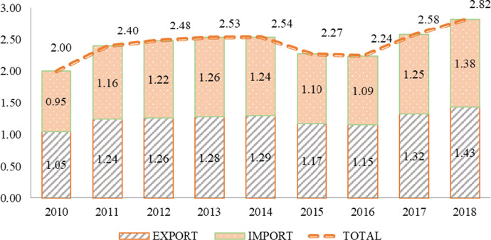
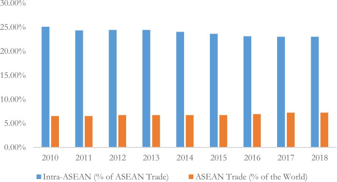
Figure 1 shows that trade in the ASEAN has increased substantially, from US$ 2 trillion in 2010 to US$ 2.82 trillion by 2018. Similarly, during the same period, export and imports increased from US$ 1.05 trillion to US$ 1.43 and US$ 0.95 trillion to US$ 1.38 trillion, respectively. Likewise, Fig. 2 shows that intra-ASEAN trade decreased over the years, from 25 in 2010 to 23% in 2018. However, the region’s contribution to world trade also increased from 5 to 7.2% during the same period. It highlights the extra-regional trade preference of the region.
Fig. 1.
ASEAN trade in goods 2010–2018 (US$ trillion). Data
source: ASEAN Integration Report (2019). This figure reports exports, imports, and total goods trade of ASEAN countries to the world
Fig. 2.
Intra-ASEAN and ASEAN (% to total world trade) 2010–2018. Data
source: ASEANstat database (retrieved Feb 2020). The figure shows the intra-ASEAN trade to total ASEAN trade and percentage of ASEAN trade to the world. The intra-ASEAN trade is between 25 and 23% from 2010 to 2018
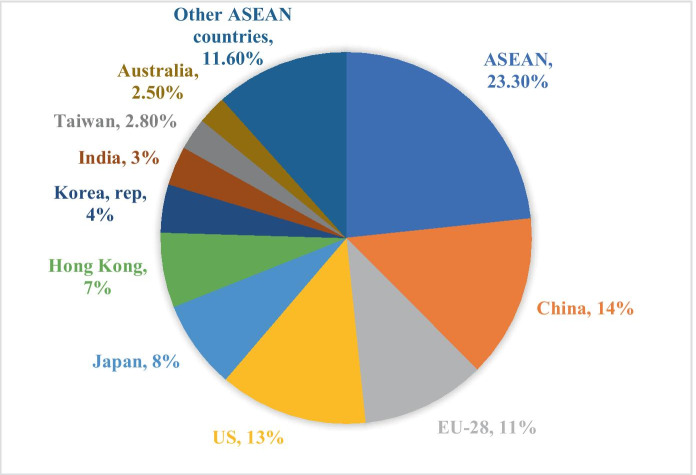
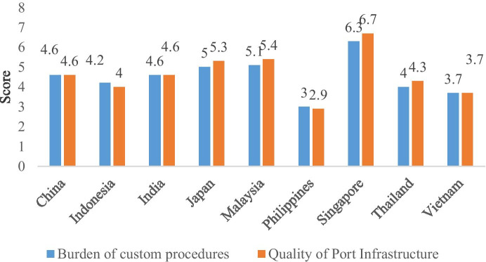
Similarly, Fig. 3 also shows that China, India, and Japan are the region’s major export destinations. In terms of port and customs procedures at the borders, we also report the quality of infrastructure in selected ASEAN countries and India, China, and Japan in Fig. 4. It clearly shows that the quality of the infrastructure varies across these countries.
Fig. 3.
Top ten export partners of ASEAN. Data
source: ASEAN statistical yearbook 2020, ASEAN Secretariat, Jakarta. This figure shows that with in bloc trade contributes around 23.3%, and hence, the members are the major partners. It is followed by China, the USA, EU, Japan, etc.
Fig. 4.
The port infrastructure and burden of custom procedures quality in selected ASEAN and India, China, and Japan in 2018. Note: quality of port is rated as 1 = extremely underdeveloped to 7 = well developed and efficient and border custom procedures: 1 = extremely inefficient to 7 = extremely efficient.
Source: World Economic Forum, Global Competitiveness Report. Accessed from WDI, 2019. The figure shows that Singapore has excellent quality of port infrastructure and less burdensome custom procedures. Malaysia and Japan are the followers with score ranging 5–5.4. Rest of all ASEAN falls below 5
Hence, this study attempts to analyze the effect of infrastructure on trade connectivity among the ASEAN, India, China, and Japan. Specifically, it addresses the following questions: (1) Are there any trade interdependence among the ASEAN and India, China, and Japan? (2) Are there any center-periphery structures in the trade network? (3) Does the infrastructure growth impact trade connectivity? (4) Do the trade cost, foreign direct investment (FDI), and regional trade agreements impact trade connectivity? We include China, Japan, and India with the ASEAN economies because (1) India and China are the world’s largest economies. They are rapidly expanding their markets and increasing their integration with the ASEAN. (2) Among the Asian giants, Japan maintains well-coordinated economic relationships in the ASEAN.
Our approach toward testing the above issues is as follows: to examine trade interconnectedness, we apply trade network analysis on these 13 countries for 1990–2018. We use network centrality parameters such as density, degree, closeness, eigenvector, betweenness, and clustering to examine trade structure. We find trade connectedness in the region and then estimate the role of the different modes of transport in supporting trade. We also construct two control variables to estimate the role of policy and foreign investments. We then apply the panel fixed effects model. Our empirical findings suggest high trade integration among the ASEAN, India, China, and Japan.
We can summarize our contributions to the existing literature as follows: first, our study is one of the rare attempts to examine the link between trade and infrastructure through the network perspective in the context of ASEAN. It supplements the existing literature on infrastructure and trade, such as Arvis and Shepherd (2011), Helble (2014), and Shepherd (2016). Second, the literature has thus far ignored the “center-periphery relationship” within the ASEAN; hence, this study also attempts to bridge this divide. Third, our finding a “trade intensive path” within the ASEAN and India, China, and Japan provides a source to frame appropriate policies in the region.
“Literature review” section in this paper reviews the literature. “Data” section presents the data, and “Methodology and empirical model” section discusses the methodology. “Results and discussion” section discusses the results, while “Conclusion and policy implications” section concludes this paper.
Literature review
We can divide the literature into four strands: (A) theoretical background, (B) network analysis and trade, (C) trade integration and its impact, and (D) role of infrastructure and trade.
Theoretical background
Economic regionalism3 theories chiefly explain the domestic factors that drive toward static and dynamic effects of economic integration in a regional level. However, the influence of external factors too turned detrimental to the development of regionalism. Balassa (1961) introduced typology of economic integration which is most widely used for theoretical and empirical discussion pertaining to regionalism and economic integration. The five forms of economic integration are free trade agreements (FTAs), customs union, common market, economic union, and monetary union. The first type is the economic cooperation among countries that rests on specific set of issues such as investment and trade.
Later in the 1990s, there came up an active debate over the impact of FTAs on the regions. One group favored the regional trade agreements (RTAs) under Summers, and the other group claimed that RTAs could be harmful and cause a threat to multilateralism in the long run under Bhagwati. From this debate, the “spaghetti bowl” theory came up. According to Bhagwati, “too many crisscrossing FTAs would allow countries to adopt discriminatory trade policies and reduce the economic benefits of trade.” And, he suggested that “coping with multiple tariffs and ROOs in FTAs can raise transaction costs for enterprises, particularly SMEs” (Kawai and Wignaraja 2009). Thus, Bhagwati et al. (1998) and Panagariya (2000) worked on the theoretical literature of FTAs and the spaghetti bowl. Later came up the insight of “ noodle bowl effect4” interpretation of the same in the context of Asian FTAs. Most of these economic integrations are based on the theoretical underpinnings of international economics. The classical and neoclassical trade theories emphasize the comparative advantage models and ignore the transport costs. However, the new trade theory identified transport cost and increasing returns as the determinants of trade patterns. Many studies have examined the importance of trade interconnectedness and its positive spillover effects (Krugman 1991; Baldwin and Okubo 2006). The Helpman and Krugman (1985) model proved the importance of scale (economies of scale) determining trade patterns. An increase in trade integration reduces countries’ geodesic distance over the years.
Network analysis and trade
Many studies discuss social and economic aspects using network analysis. This study examines the networks in the realm of international trade. Some early studies analyzed networks in the context of trade protectionism, specifically, the relationship between the “center” and “periphery” during times of high protectionism. Synder and Kick (1979) examined the world system theory and the prevailing economic system during the 1980s. However, the period after 1990 brought considerable changes in global economic systems. Globalization and technological developments have facilitated trade integration among nations. However, few studies examined binary trade networks between countries and measured trade flow to find its intensity (De Benedictis and Tajoli 2011). Kali and Reyes (2007) discussed the hierarchical structure of core and periphery positioning in global trade.
Gould et al. (2018) analyzed multidimensional connectivity using trade networks. They found that migration, internet connection, and FDI are the main channels determining growth. Arvis and Shepherd (2011) applied network connectivity to analyze the hub and spoke relationship in the air transport networks of 211 countries. In a recent study, Vidya et al. (2020) examined trade interconnectedness in a cross-country sample of 50 countries using the network model. Most recently, Vidya and Prabheesh (2020) found that world trade is changing after the COVID-19 pandemic. This study finds that the emerging economies of Asia, such as India and China, have become leaders in world trade networks. However, over the years, there is no reduction in the geodesic distance among them, which implies scant gains from trade due to trade integration.
Trade integration and its impact
Most studies on trade integration emphasize the elimination of barriers and trade costs to promote economic integration (Kahnert et al. 1969). Some studies show that trade integration promotes economic growth (Rodriguez and Rodrik 2000). Specifically, regional and preferential trade agreements improve regionalization among member countries (Frankel et al. 1995; Thangavelu and Chongvilaivan 2009). Most of these studies find that regionalization can increase the growth, competitiveness, and investments in the member countries. Some studies also highlight the prevalence of barriers for the ASEAN countries in achieving the fullest benefit from regional trade integration. One such barrier is the non-tariff barriers in the region.
Role of infrastructure on trade
Prior literature (Anderson and Wincoop 2004; Brooks and Menon 2008) has analyzed the relationship between international trade and infrastructure, finding a substantial impact on the latter. In a notable work, Nordas and Piermartini (2004) estimated the impact of the quality of infrastructure (road, airport, telecommunication, and the time required for customs clearance) on total bilateral trade and on trade in automotive, clothing, and textile sectors. The study found that port efficiency is the crucial factor among all the indicators of infrastructure. Moreover, timeliness and access to telecommunication are more important for export competitiveness. Shepherd and Wilson (2009) analyzed trade facilitation in ASEAN region and found that there is a need for reforms in trade facilitations. Expanding the port facilities can increase the trade, and hence, transport infrastructure can play a major role in enhancing intra-regional trade. Portugal-Perez and Wilson (2012) analyzed the role of physical and soft infrastructure in trade facilitation. They found that infrastructure plays a crucial role in Southeast Asian countries. Francois and Manchin (2013) and Donaubauer et al. (2018) constructed an infrastructure index and found a significant impact on trade. These infrastructure indices captured a larger set of variables—transport, communication, financial, and so on. Helble (2014) included shipping, air connectivity, and frequency, in their analysis of Pacific nations. They found that direct connectivity and frequency had a high impact on trade. Similarly, trade cost, as a proxy for tariff rates, affects trade relationships, as demonstrated by Novy (2013).
Data
This study used bilateral trade data in goods among the ASEAN countries, that is, Indonesia, Thailand, Brunei, Singapore, Philippines, Malaysia, Vietnam, Cambodia, Myanmar, and Laos. In addition, we included three Asian countries from different regions, that is, India, China, and Japan. We first estimate the network analysis to check interdependence among the ASEAN and these three countries for the continuous period of 1990–2018. We choose 1990 as the starting year of analysis because complete data is available from this year. We accessed bilateral data from the WITS World Bank database.
For network analysis, we constructed a bilateral trade matrix. The matrix is a representation of each cell showing the exports of country one to country two and its imports. We first establish trade interconnectedness and then analyze the nexus between trade connectivity and infrastructure. We then apply the panel fixed effects model for estimation purposes for the period 1990–2018 (see Table 1) for a description of our data, sources, and sample).
Table 1.
Data and variable description for the panel estimations
| Variable | Description | Definition | Source |
|---|---|---|---|
| Trade connectivity | Natural logarithm of eigenvector centrality (EVC) based on the matrix of bilateral trade flows derived using network analysis | Author’s calculations | |
| GDP per capita | Natural logarithm of per capita GDP in ppp terms | World Development Indicators (WDI) | |
| Infrastructure index | Natural logarithm of infrastructure index. The index is the PCA of 4 indicators; fixed telephone subscriptions (per 100 people), air transport (freight) million ton-km, energy use (kg of oil equivalent per capita), electric power consumption (kWh per capita) | Author’s own calculation based and WDI | |
| Trade cost | Natural logarithm of simple average of aggregate tariff | WITS-TRAINS | |
| Air transport | Natural logarithm of air transport freight (million ton-km) | WDI | |
| Power consumption | Natural logarithm of electric power consumption (kWh per capita) | WDI | |
| Shipping connectivity index | Natural logarithm of liner shipping connectivity index | WDI | |
| Foreign direct investment | Natural logarithm of FDI inflows in US$ million | WDI | |
| FDI multiplied free trade agreement | FDI and FTA is number of free trade agreements for each country specific to the region | WDI |
Methodology and empirical model
Network model estimation
To explore the trade interdependence among these countries, we first estimate the network model. We construct an undirected matrix of networks for 13 countries from 1990 to 2018. Subsequently, we adopt the following steps. An export matrix X calculated, and the value of Xij shows average exports from to and imports. We call this the “trade matrix.” Importantly, we use a trade matrix to construct an undirected network graph for the countries. Notably, an edge includes two nodes and if the value of the threshold is greater, we choose 0. We consider a threshold of 0 here.
In addition, a network model explains the nexus between different elements, such as nodes and edges. Generally, nodes act as individual actors and edges show the relationships between the nodes. Every node has an in-degree and an out-degree. An in-degree is the number of incoming edges representing the imports, while the out-degree is the number of outgoing edges, which are the exports. Table 2 provides the terms and descriptions of parameters used in the network analysis.
Table 2.
Definition of the parameters applied in network models
| Term | Description of the network parameter |
|---|---|
| Degree centrality | It shows how a node is positioned in a network and how important it is in a network structure. It represents the trade interconnectedness |
| Eigenvector centrality (EVC) |
It indicates the significance of each node to other nodes around it. In this study, the countries that show high EVC are highly connected to all the countries It represents the connectivity measure |
| Closeness centrality | The parameter that defines how much close one node to all the remaining nodes. The topological distance among the countries is mentioned here. The parameter measures the geodesic distance |
| Betweenness centrality |
The number of short paths that go through the vertex It represents the dependency |
| Density | It represents the trade density among the countries |
| Clustering coefficient | It shows the network density |
The table describes the definition and implication of the parameters used in the network model
Panel fixed effect, Poisson pseudo-maximum likelihood, and two-stage least square
The estimates of the empirical model proposed in this paper will be performed by the panel fixed effects model (country effect and time effect) at first. The various tests like Lagrange multiplier (LM) test (Breusch and Pagan 1980), F test (Moulton and Randolph 1989), likelihood ratio (LR) test (Gourieroux et al. 1982), and Hausman specification test (Hausman 1978) are carried out to understand the presence of country effect and time effect in the data and to determine fixed effects or random effects should be incorporated into the model. LM test statistics indicate that either the fixed effect country and time/time effect only or the random effect country and time/time effect only are preferred to classical linear regression model.
Moreover, Silva and Tenreyro (2006) propose the use of the Poisson pseudo-maximum likelihood (PPML) estimator because it has certain important properties compared to traditional models of OLS. First, it eliminates the sample biases and statistical problems arise due to the existence of zero trade flows. In our models, we do have bilateral cross country data set and few zero trade flows in the case of trade cost. Second, it will try in resolving the econometric problems of both efficiency and consistency that emerge in the likely presence of heteroscedastic residuals (Esteve‐Pérez et al. 2020).
We also apply two-stage least square (2SLS) method as a robustness check for the empirical model. The 2SLS helps to address the issue of endogeneity issues in a panel fixed effects model. Since many macroeconomic variables are found to be correlated with the error term, the problem of multicollinearity may arise. Thus, in the presence of multicollinearity OLS may produce spurious results. Hence, there is a need for regression model to control the correlation among the variables. To resolve the issue, several regression methods are available that may apply instruments to eliminate the effect of correlation between the independent variables and the residuals, such as 2SLS regression recommended by Cumby et al. (1983). The 2SLS model is an extension of OLS method. It can be applied in case dependent variables correlate with error term.
Empirical model
We now analyze the impact of infrastructure on trade. We estimate the following three empirical models using the panel estimation-fixed effect model. Here, the dependent variable “trade connectivity” is the eigenvector centrality derived from the network model. “Connectivity5 is considered a key ‘policy’ concept and lacks a rigorous empirical framework” (Arvis and Shepherd 2011). Hence, this study6 uses a rigorous approach to perform panel estimation on the sample.
| 1 |
| 2 |
| 3 |
The above Eqs. (1)–(3) represent bilateral trade data, where “i” stands for the home country and “j” stands for trading partner countries. Trade_Connectivity denotes the eigenvector centrality (EVC) of the bilateral trade of respective countries. EVC measures the connectivity of all the countries for the nodes in the network graphs.7GDPPC denotes GDP per capita, which is the proxy for economic development. Infra denotes the infrastructure index and we construct it using the principal component analysis (PCA) summation of four variables. These variables are as follows: fixed telephone lines (per 100 people), air transport freight in ton-km, energy use in kg of oil equivalent per capita denomination, and electric power consumption in kWh per capita. We expect a positive association between infrastructure and trade. This shows that regional infrastructure indicators such as transport, communication, and energy are important factors for trade connectivity.
Similarly, we obtain the simple average of aggregate tariff data for each country by dividing the aggregate tariff rate of each country by the sum of countries. As TC increases, trade connectivity among the countries decreases, implying a negative relationship. This variable has been taken from WITS-TRAINS database.
To minimize possible omitted variable bias on the main variables, we included the control variables and FTAit. The rationale for our selection of these variables lies in previous studies on trade and infrastructure nexus (Francois and Manchin 2013; Maurer 2009). is the FDI inflow to each country for the period 1990–2018. As FDI inflow increases, it increases the trade connectivity among countries. Similarly, FTAit shows the number of free trade agreements among the ASEAN and India, China, and Japan. FTAit is a trade policy proxy.
The second model (2) has 2 new variables in addition to the above, that is, Transport_Air and . Transport_Air denotes the air transport and freight given in million ton-kilometers. It defines the volume of freight in million tons. Similarly, . denotes the electric power consumption in each country denoted in kWh per capita. Both the variables have been availed from the WDI, World Bank. The third model (3) adds another new variable Ship_connectivity, which is the shipping connectivity index. It measures the global shipping networks of each country.
Finally, the βis in the models are the parameters to be estimated and all variables are expressed in logarithmic form (In). The detailed description of the explanatory variables and dependent variable is discussed above (Table 1).
Results and discussion
This section discusses the estimation results. We present the network analysis results and discuss them in “Results and discussion of network analysis” section, and present the panel fixed effects results in “Results and discussion—trade connectivity and its determinants” section.
Results and discussion of network analysis
We consider 13 countries in a bilateral trade matrix for the years 1990, 1992, 1995, 2000, 2005, 2010, 2015, and 2018. A visual representation of the network graphs can provide vital information on trade integration. The complete results from 1990 to 2018 are difficult to present in this paper because of their complexity. Therefore, we show the network parameters of certain years in Table 3 and include the full period of study from 1992 to 2018 and the full series in Table 4.
Table 3.
Parameters of network analysis
| Year | Density | Degree centrality | Eigenvector centrality | Betweenness centrality | Closeness centrality | Clustering coefficient |
|---|---|---|---|---|---|---|
| 1990 | 0.679 | 0.662 | 0.269 | 0.029 | 0.788 | 0.843 |
| 1992 | 0.679 | 0.679 | 0.269 | 0.029 | 0.788 | 0.843 |
| 1995 | 0.795 | 0.795 | 0.273 | 0.019 | 0.855 | 0.874 |
| 2000 | 0.962 | 0.962 | 0.277 | 0.003 | 0.967 | 0.965 |
| 2005 | 0.962 | 0.962 | 0.277 | 0.003 | 0.967 | 0.965 |
| 2010 | 0.868 | 0.929 | 0.277 | 0.012 | 0.934 | 0.988 |
| 2015 | 0.879 | 0.941 | 0.277 | 0.012 | 0.934 | 0.988 |
| 2018 | 0.846 | 0.905 | 0.277 | 0.009 | 0.907 | 0.980 |
This table discusses the results of parameters of network analysis. Source: Author’s analysis using network models
Table 4.
Parameters of network analysis, 1990–2018
| Year | Density | Degree centrality | Eigenvector centrality | Betweenness centrality | Closeness centrality | Clustering coefficient |
|---|---|---|---|---|---|---|
| 1990 | 0.679 | 0.662 | 0.269 | 0.029 | 0.788 | 0.843 |
| 1991 | 0.679 | 0.679 | 0.269 | 0.029 | 0.788 | 0.843 |
| 1992 | 0.758 | 0.811 | 0.275 | 0.024 | 0.846 | 0.898 |
| 1993 | 0.846 | 0.980 | 0.274 | 0.014 | 0.886 | 0.897 |
| 1994 | 0.859 | 0.859 | 0.274 | 0.013 | 0.895 | 0.902 |
| 1995 | 0.795 | 0.795 | 0.273 | 0.019 | 0.855 | 0.874 |
| 1996 | 0.859 | 0.859 | 0.274 | 0.013 | 0.895 | 0.902 |
| 1997 | 0.923 | 0.978 | 0.276 | 0.007 | 0.938 | 0.937 |
| 1998 | 0.910 | 0.910 | 0.276 | 0.008 | 0.929 | 0.931 |
| 1999 | 0.872 | 0.872 | 0.275 | 0.012 | 0.904 | 0.907 |
| 2000 | 0.962 | 0.962 | 0.277 | 0.003 | 0.967 | 0.965 |
| 2001 | 0.857 | 0.917 | 0.277 | 1.551 | 0.925 | 0.976 |
| 2002 | 0.987 | 0.987 | 0.277 | 0.001 | 0.988 | 0.987 |
| 2003 | 0.987 | 0.987 | 0.277 | 0.001 | 0.988 | 0.987 |
| 2004 | 0.987 | 0.987 | 0.277 | 0.001 | 0.988 | 0.987 |
| 2005 | 0.962 | 0.962 | 0.277 | 0.003 | 0.967 | 0.965 |
| 2006 | 0.987 | 0.987 | 0.277 | 0.001 | 0.988 | 0.987 |
| 2007 | 0.987 | 0.987 | 0.277 | 0.001 | 0.988 | 0.987 |
| 2008 | 0.987 | 0.987 | 0.277 | 0.001 | 0.988 | 0.987 |
| 2009 | 0.987 | 0.987 | 0.277 | 0.001 | 0.988 | 0.987 |
| 2010 | 0.868 | 0.929 | 0.277 | 0.012 | 0.934 | 0.988 |
| 2011 | 0.868 | 0.929 | 0.277 | 0.012 | 0.934 | 0.988 |
| 2012 | 0.868 | 0.929 | 0.277 | 0.012 | 0.934 | 0.988 |
| 2013 | 0.868 | 0.929 | 0.277 | 0.012 | 0.934 | 0.988 |
| 2014 | 0.879 | 0.941 | 0.277 | 0.012 | 0.934 | 0.988 |
| 2015 | 0.879 | 0.941 | 0.277 | 0.012 | 0.934 | 0.988 |
| 2016 | 0.868 | 0.929 | 0.277 | 0.012 | 0.934 | 0.988 |
| 2017 | 0.857 | 0.917 | 0.277 | 0.013 | 0.925 | 0.976 |
| 2018 | 0.846 | 0.905 | 0.277 | 0.008 | 0.907 | 0.985 |
Source: Author’s own calculations
Trade density improved from 0.679 in 1990 to 0.846 in 2018. This highlights the increasing trade density among the ASEAN and India, China, and Japan.
Similarly, degree centrality (DC) measures trade interconnectedness. The DC is between 0 and 1. The DC of the ASEAN and India, China, and Japan increased from 1990 to 2018 (see Table 3). The value in 1990 was about 0.662, which spiked to 0.795 in 1995; it then rose to 0.962 during 2000 to 2005. The high degree centrality is due to higher trade reciprocity and there are several RTAs among the ASEAN and India, China, and Japan.
During 1990, the closeness centrality was around 0.788, increasing to 0.967 by 2000 and to 0.907 by 2018. This implies that geodesic distance has decreased among the ASEAN and India, China, and Japan. Therefore, the countries have become closer over the years.
Similarly, the eigenvector centrality explains the connectivity measure. The median value in 1990 is 0.269; in 2000, it is 0.277, and until 2018, the value remains unchanged at 0.277. The metric is almost stable from 2000 to 2018. Hence, countries that trade closely in the region remain well connected within the region, but not with the rest of the region. Explicitly, trade connectivity became centripetal in the ASEAN.
The betweenness centrality, which represents dependency, fell to 0.029 in 1990 and to 0.003 in 2000. Later, the metric caught up to 0.012 (2010–2015); however, it fell again to 0.009 in 2018. This indicates growing trade integration in the region. The theory states that high betweenness centrality implies that a country is playing an important role in connecting other countries, probably as an intermediary that consumes raw materials and produces finished goods (Zhao 2017). In this study, Japan, Thailand, Singapore, Malaysia, and China act as export hubs and suppliers of intermediate goods.
Similarly, network density is depicted as a clustering coefficient. Network density was around 0.843 during 1990; it increased to 0.965 in 2000 and 0.980 in 2018. This indicates growing regional trade integration and trade interconnectedness. Therefore, trade integration before and after ASEAN-108 shows that trade intensity among the member countries increased substantially after 2000. Trade relationships among the member countries and Japan, India, and China became denser, interconnected, and grew close over the years. Importantly, trade in the region turned asymmetric and highly regionalized. In fact, trade connectivity became centripetal in the ASEAN.
The results from the EVC are from the bilateral trade links (see Table 5). During 1990, the highest connectivity score was for India, Japan, Thailand, and Malaysia, and the least connectivity score was for Brunei, Vietnam, Cambodia, and Laos. The post-trade liberalization (post-1995) saw tangible improvement in connectivity in intra-regional trade. Except for Brunei, almost all the ASEAN and India, China, and Japan improved their trade connectivity. In 2015, Myanmar made drastic changes to its connectivity trends.
Table 5.
Eigenvector centrality (connectivity) for bilateral trade in goods, 1990–2018
| Country | 1990 | 1992 | 1995 | 2000 | 2005 | 2010 | 2015 | 2018 |
|---|---|---|---|---|---|---|---|---|
| India | 0.35 | 0.30 | 0.32 | 0.29 | 0.29 | 0.28 | 0.28 | 0.28 |
| Japan | 0.35 | 0.30 | 0.32 | 0.29 | 0.29 | 0.28 | 0.28 | 0.28 |
| Malaysia | 0.35 | 0.30 | 0.32 | 0.29 | 0.29 | 0.28 | 0.28 | 0.28 |
| Thailand | 0.35 | 0.30 | 0.32 | 0.29 | 0.29 | 0.28 | 0.28 | 0.28 |
| Indonesia | 0.33 | 0.30 | 0.30 | 0.29 | 0.29 | 0.28 | 0.28 | 0.28 |
| Singapore | 0.29 | 0.30 | 0.32 | 0.29 | 0.29 | 0.28 | 0.28 | 0.28 |
| China | 0.23 | 0.30 | 0.32 | 0.29 | 0.29 | 0.28 | 0.28 | 0.28 |
| Myanmar | 0.23 | 0.27 | 0.22 | 0.25 | 0.25 | 0.28 | 0.30 | 0.31 |
| Philippines | 0.23 | 0.22 | 0.22 | 0.29 | 0.29 | 0.28 | 0.28 | 0.28 |
| Cambodia | 0.20 | 0.22 | 0.22 | 0.29 | 0.29 | 0.28 | 0.28 | 0.24 |
| Lao PDR | 0.20 | 0.20 | 0.22 | 0.25 | 0.25 | 0.28 | 0.28 | 0.24 |
| Vietnam | 0.20 | 0.25 | 0.22 | 0.29 | 0.29 | 0.28 | 0.28 | 0.24 |
| Brunei | 0.19 | 0.27 | 0.19 | 0.25 | 0.25 | 0.28 | 0.28 | 0.28 |
The table shows indicator of a country’s overall place in the world trade network. Source: Author’s analysis
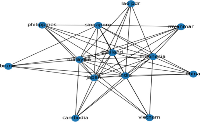
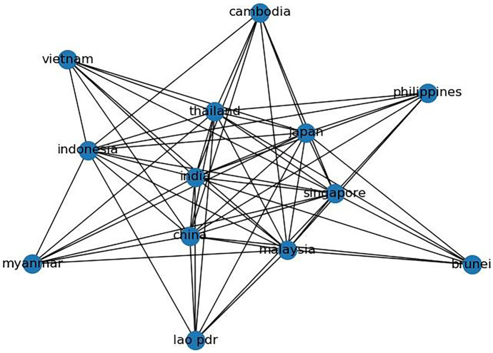
Figure 5 shows the network graphs of ASEAN and India, China, and Japan for the year 1990. During 1990, the countries in the center are Thailand, Malaysia, Japan, and India. The periphery includes Brunei, Philippines, Singapore, Lao, Cambodia, Indonesia, Myanmar, China, and Vietnam. Strikingly, the map reveals a thick black line passing through some countries. We term these “trade intensive paths.” This path starts from Singapore, passes through Thailand, reaches India, and then stretches to Vietnam. The networks highlight the trade connections and emergence of within interconnections.
Fig. 5.
Network of trade in goods, 1990.
Source: Author’s analysis
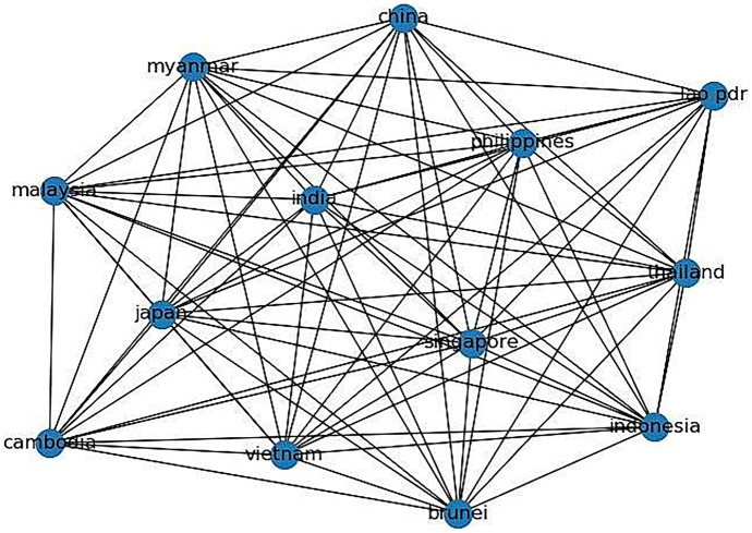
We plot the immediate year, 1992 (Fig. 6), to show a complex network graph. In the 1990s, most countries in Asia began to liberalize their markets. Trade openness and liberalization helped expand and diversify trade across borders. India, Singapore, Japan, Philippines, and Vietnam are in the center of the networks. The trade intensive path goes through China, Japan, and Cambodia.
Fig. 6.
Network of trade in goods, 1992.
Source: Author’s analysis
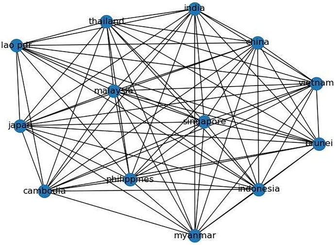
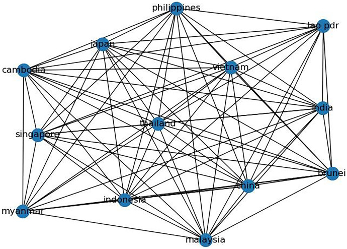
Noticeably, by 2000 (Fig. 7), there was a substantial change in trade connectivity. Malaysia and Singapore concentrated toward the center and became the main centrifugal forces in deciding trade relationships. Although we can see multiple thick lines (trade intensive paths) on the map, the most prominent among them is Thailand-Malaysia-Philippines-India. Another striking feature of the trade connectivity map of 2005 is the leadership of Thailand. Thailand became the core or dominant country in the ASEAN and India, China, and Japan. Figure 8 shows that most of the nodes and edges passed through Thailand, implying its emergence as a reliable trade partner for many. We may also consider it an export hub supplying raw materials.
Fig. 7.
Network of trade in goods, 2000.
Source: Author’s analysis
Fig. 8.
Network of trade in goods, 2005.
Source: Author’s analysis
Figure 9 presents the map of 2015. The nodes and edges in the trade network became denser but less complicated. The 2015 map is more symmetric and definite in the relationships among countries than the previous trade networks. There emerged clearer and visible trade intensive paths by 2015. Some of the explicit routes are (i) Cambodia-Thailand-India-China, (ii) Japan-Singapore-Thailand, (iii) Japan-India-Thailand, and (iv) Thailand-Malaysia-Japan.
Fig. 9.
Network of trade in goods, 2015.
Source: Author’s analysis
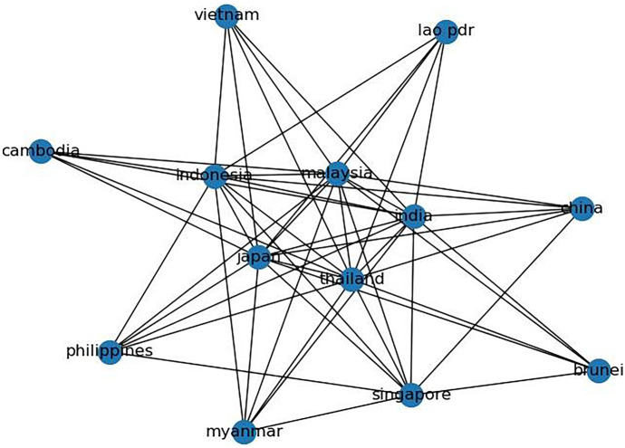
The most recent trade network map is of 2018 (see Fig. 10). Unlike the previous maps, it represents a more transparent and distinct trade interconnection. The center countries in the network are Indonesia, Japan, Thailand, India, and Malaysia. We presume the trade intensive paths to be (i) Indonesia-Japan-Malaysia, (ii) Japan-Malaysia-Thailand, and (iii) Malaysia-Thailand-India.
Fig. 10.
Network of trade in goods, 2018.
Source: Author’s analysis
Results and discussion—trade connectivity and its determinants
Table 6 shows the results of three basic tests conducted as a primary step before proceeding to the panel data model. The tests are likelihood ratio (LR), F-test, and the Hausman specification test. The results of the LR and F-test indicate that the null hypotheses and are rejected at the 1% level of significance; therefore, both country and time effect are present in the data. The Hausman specification test is significant at the 1% level (Table 7). The null hypothesis stating that individual country specific effects are uncorrelated with the regressors in the model is rejected. Hence, we conclude that the fixed effect model is preferable over the random effect model. The results of the panel unit root in Table 8 do not show any evidence of non-stationarity.
Table 6.
LR and F-test results for the significance of the country and time effect
| Type of test | P-value | Model 2 | P-value | Model 3 | P-value | |||
|---|---|---|---|---|---|---|---|---|
| LR | χ2(01) = 261.08 | 0.00 | LR | χ2(01) = 178.95 | 0.00 | χ2(01) = 4.04 | 0.00 |
Table 7.
Panel fixed effects model
| Variables | Model 1 | Model 2 | Model 3 |
|---|---|---|---|
|
0.340* (0.113) |
|||
|
0.017* (0.006) |
0.011* (0.003) |
||
|
− 0.177* (0.018) |
− 0.218* (0.019) |
− 0.118* (0.031) |
|
|
0.017* (0.006) |
|||
|
0.072* (0.020) |
|||
|
0.022** (0.011) |
|||
|
0.575* (0.232) |
|||
|
0.005* (0.002) |
|||
| Constant |
1.520* (0.123) |
1.942* (0.152) |
0.730* (0.131) |
| N | 279 | 279 | 279 |
| 0.28 | 0.32 | 0.32 | |
| F-stat | 14.29 [0.00] | 13.13 [0.00] | 9.74 [0.00] |
| Hausman spec | 17.89 [0.00] | 20.66 [0.00] | 129.50 [0.00] |
*, **, and *** denote statistical significance at the 1%, 5%, and 10% levels, respectively
Values in parenthesis and square brackets indicate standard errors and level significance
Table 8.
Panel unit root—Results (Im-Pesaran-Shin)
| Variables | Statistics (P-value) |
|---|---|
| − 4.541 (0.00)* | |
| − 6.823 (0.00)* | |
| − 4.3172 (0.00)* | |
| − 2.887 (0.00)* | |
| − 3.413 (0.00)* | |
| − 5.29 (0.00)* | |
| − 6.75 (0.00)* |
* and ** indicate significance levels at 1% and 5%, respectively
Our estimates begin with the fixed effects model results presented in Table 4. We estimated the variables in a step-by-step manner so as to avoid any harmful collinearity between variables. In column 2, we introduced , , and . The variable has a positive relationship with trade connectivity, indicating that a rise in GDP per capita positively impacts trade connectivity among the countries. Similarly, the variable infrastructure index shows positive and significant impact on trade connectivity. Hence, the development of hard infrastructure is crucial for trade connectivity. This is similar to the findings of Francois and Manchin (2013).
Conversely, the trade cost, which represents the simple average tariff bilateral tariff rates among the countries in the region, shows a negative and significant impact. The results show that an increase in trade cost negatively affects trade connectivity among the countries. The variable shows significant but negative and a very small percentage change in trade connectivity. The theoretical underpinning (Krugman 1991) is that a reduction in trade costs leads to more geographical concentration of production and trade integration. Importantly, when trade costs of the intermediate inputs drop substantially, it facilitates fragmented trade in different locations of the region (WTO 2008).
In the second model in column 3, we introduced and as a separate variables to capture the infrastructural development of the regions. Hence, there are four variables altogether in the 2nd model— and , and . The infrastructural variables (air transport and power) are positive and significant. However, they show a very small amount of change in the dependent variable. Apart from the infrastructural variables, we have included control variables . As expected, they are positive and significant. The coefficient FDI influences the host countries in multiple ways, such as the development of multinational firms in the host country, technological development, and infrastructural development. Thus, the positive spillover benefits the acceleration of strong trade connectivity. Similarly, the interaction of FDI with FTA reveals policy implications. The ASEAN have a high number of FTAs. The impact of more FTAs among the ASEAN and India, China, and Japan has encouraged more FDI, contributing to trade growth.
The third model is given in the 4th column of the table. It highlights that infrastructure index and shipping connectivity shows positive and significant change. To capture the benefits of policy, we include an interaction term free trade agreement () with . The positive and significant interaction term conveys that trade agreements play a crucial role in bringing foreign investments and facilitating better trade connectivity.
We have re-estimated the model using PPML to rule out any biases and to resolve the zero trade flows in the bilateral trade. The results are almost in line with the fixed effects model with minor changes and given in Table 9. The model has been estimated in the same step-wise manner. It is important to note that, in model 2 and model 3, the infrastructural development index () which is a proxy for all the major hard infrastructures of ASEAN and the three shows more pronounced values. One percent increase in the trade connectivity increases the infrastructure of the region by 1.36%, indicating the importance of the same as the major determinant. Similarly, the trade cost also shows better results compared to FE model.
Table 9.
Poisson pseudo-maximum likelihood (PPML) model
| Variables | Model 1 | Model 2 | Model 3 |
|---|---|---|---|
|
0.244 (0.146) |
|||
|
0.036* (0.003) |
0.0557** (0.028) |
||
|
− 0.800* (0.030) |
− 0.642* (0.192) |
− 0.516* (0.146) |
|
|
0.0752* (0.0187) |
|||
|
0.368 (0.614) |
|||
|
0.594* (0.206) |
|||
|
0.376** (0.148) |
|||
|
0.006 (0.087) |
|||
| Constant |
7.37* (2.431) |
4.86* (2.611) |
0.730* (0.131) |
| N | 279 | 279 | 279 |
| 0.216 | 0.297 | 0.187 |
*, **, and *** denote statistical significance at the 1%, 5%, and 10% levels, respectively
Values in parenthesis and square brackets indicate standard errors and level significance
Finally, in Table 10, we report the findings from the robustness test based on a two-stage least square (2SLS). This methodology takes into account any endogenous issue between the variables in the model. The findings from the 2SLS estimation do not alter the overall conclusion.
Table 10.
Robustness check—2-stage least squares (2SLS)
| Variables | Model 1 | Model 2 | Model 3 |
|---|---|---|---|
|
0.340* (0.11) |
|||
|
0.0228* (0.003) |
|||
|
0.490* (0.043) |
0.329* (0.058) |
0.262* (0.003) |
|
|
0.146 (0.22) |
|||
|
0.394 (0.45) |
|||
|
1.170 (0.80) |
|||
|
0.575* (0.23) |
|||
|
0.026 (0.029) |
|||
| Constant |
10.07* (2.29) |
30.46* (9.44) |
12.573* (5.3) |
| N | 206 | 101 | 101 |
| 0.28 | 0.32 | 0.32 | |
| Under identification test (Anderson canon. corr. LM statistic,(Chi-sq)) | 68.02* | 44.65* | 21.27* |
| Weak identification test (Cragg-Donald Wald F statistic) | 68.35* | 24.83* | 19.93* |
|
Sargan statistic (over identification test of all instruments)/Hansen J statistic (Chi-sq) |
6.35* | 21.16* | 6.65* |
|
Endogeneity test of endogenous regressors (Chi-sq) |
22.18* | 17.22* | 15.34* |
*, **, and *** denote statistical significance at the 1%, 5%, and 10% levels, respectively. Values in parenthesis indicate standard errors
Conclusion and policy implications
The study investigated the trade interconnectedness of ASEAN economies and the nexus between infrastructure and trade connectivity. We considered 13 countries—ASEAN and three selected partners (India, China, and Japan) for the period 1990 to 2018. We used network analysis to estimate trade interdependence and the panel fixed effects, PPML model to estimate the determining factors of trade connectivity.
Our findings confirm the growing trade integration among ASEAN and India, China, and Japan. Trade density and interdependence have increased substantially since 1990. However, there is no dominant center and periphery within the region. Many developing countries in the region have come to the center. During 1990, India, Japan, Indonesia, Malaysia, Thailand, and Singapore were in the center. However, by the mid-1990s, many developing economies, such as the Philippines, Myanmar, and Vietnam, approached the center of the trade networks. Hence, trade integration has benefited the developing economies of ASEAN and India, China, and Japan. Trade integration and intensity increased substantially after 2000. The trade relationship of ASEAN with India, China, and Japan improved significantly.
Moreover, the study finds “trade intensive paths” within the region, as per the network maps. A prominent path is Thailand-Malaysia-Japan. Noticeably, the emergence of Thailand as a leader is notable. Thailand is the only country in the center in most network maps for the period 1990–2018. Specifically, during 1990, 2005, 2015, and 2018, Thailand was positioned as a center. Similarly, India approached the center in 1992, 2015, and 2018.
In terms of other network maps’ parameters, we find that trade density has increased substantially. The geodesic distance among the ASEAN and India, China, and Japan has decreased over the years. Importantly, the closeness among the countries has narrowed. Trade interlinkage is dense, and hence, a strong trade regionalization. The high degree of centrality is due to the increased trade reciprocity and the RTAs and FTAs in the region and with India, China, and Japan. The countries are well connected within the region but not with the rest of the region. Explicitly, trade connectivity has become centripetal in the ASEAN. In this study, Japan, Thailand, Singapore, Malaysia, and China act as export hubs and intermediate goods suppliers.
Our second analysis connected trade connectivity and infrastructural development; for this, we first estimated the fixed effect panel model. As the fixed effects model may not capture the zero trade flows and may bias the estimation, the study applied the PPML model. The study also conducted the robustness check using 2SLS to check the endogeneity issue with the model. We found a positive relationship between connectivity and infrastructure. We also found that trade cost (a proxy for trade barriers) negatively affects trade connectivity.
Similarly, air transport and shipping connectivity play a crucial role in increasing trade connectivity. Apart from infrastructural developments, reducing tariffs and non-tariff barriers is equally important in reducing trade costs. Reduction in trade costs can enhance trade facilitation and future trade prospects for the region. Increasing trade fragmentation promotes barrier-free markets and reduces cost and time at the borders. Hence, technology plays a crucial role in digitization and better trade connectivity. We recommend developing quality infrastructure and investment in soft infrastructure (trade facilitation programs). This study finds that the ASEAN and India, China, and Japan are export hubs for intermediate markets within the region; they can expand connectivity beyond the region too. The ASEAN and India, China, and Japan can develop the region as both exporters and suppliers for Asia and Europe. We argue that given the high intra-regional trade connectivity among the ASEAN, policymakers in this region should consider “trade intensive paths” to position the production and supply among the ASEAN and its leading partners.
Acknowledgements
This paper was presented in the Asian Development Bank Institute, Tokyo, webinar/workshop on “Energy and Transport Infrastructure Connecting Asia and Europe: Investment, Transportation, Trade & COVID-19” on 27–29 May 2020. The authors are grateful to the participants of the webinar, the Editor in Chief of the Asia-Europe Journal, and the anonymous reviewers for providing us with constructive comments that helped us to revise the paper and prepare the current version.
Appendix
Declarations
Competing interests
The authors declare no competing interests.
Footnotes
As per May 2019, 99.3% of all tariffs have been eliminated by the ASEAN-6.
See for details ASEAN Integration Report 2019, ASEAN Secretariat, Jakarta.
Economic integration refers to both institutionalized economic structure established by regional agreements (regionalism) and the process/status of integration driven by trade and investments (regionalization). The term regionalism, of which its origins are found in international relations, refers to any form of institutionalized regional cooperation involving more than two countries. Distinguished from regionalism, the term regionalization refers to an intensification of trade and investments at an intra-regional level (see for details Kang 2016).
Introduced by President Haruhiko Kuroda of the Asian Development Bank in July 2006 in a speech delivered to the Jeju Summer Forum in South Korea (Bhagwati 2008) as cited in Kawai and Wignaraja (2009).
The description of “connectivity” “An intrinsic characteristic of ‘connectivity’ is it is synonymous with the networks, which consists of interconnected nodes. Therefore, connectivity is an attribute of a network and which is a measure of how well connected anyone node other nodes in the network” (World Bank-OECD 2019; PP:1) https://www.oecd.org/g20/summits/osaka/G20-DWG-Background-Paper-Infrastructure-Connectivity.pdf.
In this section, we modeled the estimation in line with Shepherd (2016).
De Benedictis et al. (2014) and (Shepherd 2016) have used EVC, which measures each country’s position in the trade network.
ASEAN-10 formed on April 30, 1999.
Publisher's Note
Springer Nature remains neutral with regard to jurisdictional claims in published maps and institutional affiliations.
References
- Anderson J, Wincoop VE. Trade costs. J Econ Lit. 2004;42:691–751. doi: 10.1257/0022051042177649. [DOI] [Google Scholar]
- Arvis J, Shepherd B (2011) The air connectivity index: measuring integration in the global air transport network. The World Bank policy research
- Balassa B (1961)The theory of economic integration. Homewood: Richard Irwin
- Baldwin RE, Okubo T. Heterogeneous firms, agglomeration and economic geography: spatial selection and sorting. J Econ Geogr. 2005;6:323–346. doi: 10.1093/jeg/lbi020. [DOI] [Google Scholar]
- Bhagwati J, Greenaway D, Panagariya A. Trading preferentially: theory and policy. Econ j. 1998;108:1128–1148. doi: 10.1111/1468-0297.00334. [DOI] [Google Scholar]
- Bhagwati J (2008) Termites in the Trading System: How Preferential Agreements Undermine Free Trade. Oxford: Oxford University Press
- Breusch TS, Pagan AR. The Lagrange multiplier test and its applications to model specification in econometrics. Rev Econ Stud. 1980;47:239–253. doi: 10.2307/2297111. [DOI] [Google Scholar]
- Brooks DH. Regional cooperation, infrastructure and trade costs in Asia in the book trade facilitation and regional cooperation in Asia. Asian Development Bank Institute (ADBI) 2010 doi: 10.4337/9781849806527.00005. [DOI] [Google Scholar]
- Brooks DH, Menon J. Infrastructure and trade in Asia. United Kingdom: Edward Elgar Publishing; 2008. [Google Scholar]
- Cumby RE, Huizinga J, Obstfeld M. Two-step two-stage least squares estimation in models with rational expectations. J Econ. 1983;21:333–355. doi: 10.1016/0304-4076(83)90049-0. [DOI] [Google Scholar]
- De Benedictis L, Tajoli L. The world trade network. The World Econ. 2011;34:1417–1454. doi: 10.1111/j.1467-9701.2011.01360.x. [DOI] [Google Scholar]
- De Benedictis L, Nenci S, Santoni G, Tajoli L, Vicarelli C. Network analysis of world trade using the BACI-CEPII dataset. Global Eco Journal. 2014;14:287–343. doi: 10.1515/gej-2014-0032. [DOI] [Google Scholar]
- Donaubauer J, Glas A, Meyer B, Nunnenkamp P. Disentangling the impact of infrastructure on trade using a new index of infrastructure. Rev World Econ. 2018;154:745–784. doi: 10.1007/s10290-018-0322-8. [DOI] [Google Scholar]
- Esteve-Pérez G-P, Llorca-Vivero R, Martínez-Serrano JA. EMU and trade: a PPML re-assessment with intra-national trade flows. The World Eco. 2020;43:2574–2599. doi: 10.1111/twec.12960. [DOI] [Google Scholar]
- Francois J, Manchin M. Institutions, infrastructure, and trade. World Dev. 2013;46:165–175. doi: 10.1016/j.worlddev.2013.02.009. [DOI] [Google Scholar]
- Frankel J, Stein E, Wei SJ (1995) Trading blocs and the Americas: the natural, the unnatural, and the super-natural. J Dev Econ 47:61–95
- Gould D, Kenett DY, Panterov G. Multidimensional connectivity: benefits, risks, and policy implications for Europe and Central Asia. The World Bank. 2018 doi: 10.1596/1813-9450-8438. [DOI] [Google Scholar]
- Gourieroux C, Holly A, Monfort A (1982) Likelihood ratio test, Wald test, and Kuhn-Tucker test in linear models with inequality constraints on the regression parameters.Econometrica 63–80
- Hausman JA (1978) Specification tests in econometrics. Econometrica 1251–1271
- Helble M (2014) The Pacific’s connectivity and its trade implications, working paper.Asian Development Bank. https://doi.org/https://www.adb.org/sites/default/files/publication/156354/adbi-wp499.pdf
- Helpman E, Krugman P (1985) Increasing returns, imperfect competition, and international trade. MIT Press, Cambridge. https://doi.org/http://documents1.worldbank.org/curated/en/859151468161649899/pdf/WPS5722.pdf
- Kahnert FP, Richards E, Stoutjesdijk, Thomopoulos P (1969) Economic integration among developing countries. Paris: Development Center of the Organization for Economic Co-operation and Development (OECD)
- Kali R, Reyes J. The architecture of globalization: a network approach to international economic integration. J Int Bus Stu. 2007;38:595–620. doi: 10.1057/palgrave.jibs.8400286. [DOI] [Google Scholar]
- Kang YD (2016) Development of regionalism: new criteria and typology. J Econ Integr 234–274
- Kawai M, Wignaraja G (2009) The Asian noodle bowl: is it serious for business? Working paper series no. 135 Asian Development Bank, Manila
- Krugman PR. Geography and trade. Cambridge, MA: MIT Press; 1991. [Google Scholar]
- Maurer J (2009) The effects of foreign direct investment in urban development: The case of Budapest. Development Planning Unit, University College London
- Moulton BR, Randolph WC. Alternative tests of the error components model. Econometrica. 1989;57:685–693. doi: 10.2307/1911059. [DOI] [Google Scholar]
- Nordas H, Piermartini R (2004) Infrastructure and trade, Staff working paper series, Economics Research and Statistics Division, World Trade Organization, Geneva
- Novy D. Gravity redux: measuring international trade costs with panel data. Econ Inq. 2013;51:101–121. doi: 10.1111/j.1465-7295.2011.00439.x. [DOI] [Google Scholar]
- Panagariya A (2000) Preferential Trade Liberalization: The Traditional Theory and New Developments. J Econ Lit. 38(2):287–331
- Portugal-Perez A, Wilson JS. Export performance and trade facilitation reform: hard and soft infrastructure. World Dev. 2012;40:1295–1307. doi: 10.1016/j.worlddev.2011.12.002. [DOI] [Google Scholar]
- Rodriguez F, Rodrik D. Trade policy and economic growth: a skeptic’s guide to the cross-national evidence. NBER Macroecon Annu. 2000;15:261–325. doi: 10.1086/654419. [DOI] [Google Scholar]
- Roland-Holst D (2006) Infrastructure as a catalyst for regional integration, growth, and economic convergence: scenario analysis for Asia. Economics and research department working paper series no. 91, Asian Development Bank, Manila
- Shepherd B. Infrastructure, trade facilitation, and network connectivity in sub-Saharan Africa. J Afr Trade. 2016;3:1–22. [Google Scholar]
- Shepherd B, Wilson JS (2009) Trade facilitation in ASEAN member countries: Measuring progress and assessing priorities. J Asian Econ, 20(4), 367–383
- Silva JS, Tenreyro S. The log of gravity. Rev Econ Stat. 2006;88:641–658. doi: 10.1162/rest.88.4.641. [DOI] [Google Scholar]
- Snyder D, Kick EL. Structural position in the world system and economic growth, 1955–1970: a multiple-network analysis of transnational interactions. Am J Sociol. 1979;84:1096–1126. doi: 10.1086/226902. [DOI] [Google Scholar]
- Thangavelu S, Chongvilaivan A (2009) Free trade agreements, regional integration and growth in ASEAN. National University of Singapore
- Vidya CT, Prabheesh KP. Implications of COVID-19 pandemic on the global trade networks. Emerg Mark Financ Tr. 2020;56:2408–2421. doi: 10.1080/1540496X.2020.1785426. [DOI] [Google Scholar]
- Vidya CT, Prabheesh KP, Sirowa S. Is trade integration leading to regionalization? Evidence from Cross-Country Network Analysis, J Econ Integr. 2020;35:10–38. [Google Scholar]
- World Bank-OECD (2019) Infrastructure connectivity, Japan G20 Development Working Group. Prepared for OECD, Organization for Economic Cooperation and Development. Accessed online website https://www.oecd.org/g20/summits/osaka/G20-DWG-Background-Paper-Infrastructure-Connectivity.pdf on 14th June 2020
- World Trade Organization (2008) World trade report. World Trade Organization
- Zhao C. International trade and economic growth: a network perspective, unpublished Master’s thesis. Texas, United States: Baylor University; 2017. [Google Scholar]


