Knowledge extraction and transfer in data-driven fracture mechanics

Significance

Data-driven approaches have launched a new paradigm in scientific research that is bound to have an impact on all disciplines of science and engineering. However, at this juncture, the exploration of data-driven techniques in the century-old field of fracture mechanics is highly limited, and there are key challenges including accurate and intelligent knowledge extraction and transfer in a data-limited regime. Here, we propose a framework for data-driven knowledge extraction in fracture mechanics with rigorous accuracy assessment which employs active learning for optimizing data usage and for data-driven knowledge transfer that allows efficient treatment of three-dimensional fracture problems based on two-dimensional solutions.

Abstract

Data-driven approaches promise to usher in a new phase of development in fracture mechanics, but very little is currently known about how data-driven knowledge extraction and transfer can be accomplished in this field. As in many other fields, data scarcity presents a major challenge for knowledge extraction, and knowledge transfer among different fracture problems remains largely unexplored. Here, a data-driven framework for knowledge extraction with rigorous metrics for accuracy assessments is proposed and demonstrated through a nontrivial linear elastic fracture mechanics problem encountered in small-scale toughness measurements. It is shown that a tailored active learning method enables accurate knowledge extraction even in a data-limited regime. The viability of knowledge transfer is demonstrated through mining the hidden connection between the selected three-dimensional benchmark problem and a well-established auxiliary two-dimensional problem. The combination of data-driven knowledge extraction and transfer is expected to have transformative impact in this field over the coming decades.

Data-driven approaches, e.g., machine learning (ML), have emerged as a new paradigm in scientific research (1–11). So far there is very little understanding in two essential components of the data-driven approaches, knowledge extraction and transfer, in the century-old engineering discipline of fracture mechanics. Here knowledge generally includes both qualitative and quantitative understanding of a physical phenomenon, as well as the connection between different physical problems. Interestingly, both knowledge extraction and transfer have been involved extensively in the historical development of fracture mechanics. For example, size-dependent fracture strength was originally observed in experiments. Exactly a century ago Griffith invoked the laws of thermodynamics and formulated a quantitative fracture theory which connects the fracture strength and flaw size in brittle materials (12). Weibull built on Griffith’s work and formulated the statistical nature and specimen-size dependence of fracture strength by assuming a probabilistic distribution of the largest flaw size (13). This statistical theory of size effect was adapted and “transferred” by Bažant and Planas in the study of quasi-brittle fracture (14, 15).

Indeed, using advanced ML algorithms, valuable knowledge can be extracted from experimental or computational data on fracture-related problems, as shown in some prior work (4–11). However, these studies rely on limited datasets due to practical issues associated with the generation of large amounts of data. Data scarcity is a common challenge that raises the concern of knowledge bias, as the accuracy cannot be correctly assessed without sufficient data. On the other hand, it is imperative to incorporate rigorous accuracy assessment in knowledge extraction, even when the quantity of data is limited. Moreover, there have been no studies on knowledge transfer in the context of data-driven fracture mechanics. It is still unclear how to implement ML-based knowledge transfer between different fracture mechanics problems.

Here, we propose a data-driven framework for knowledge extraction in fracture mechanics, with particular emphasis on accuracy assessment. The applicability of the proposed framework is demonstrated through a specific example problem encountered in small-scale fracture toughness measurements. This specific problem requires a predictive model in which accuracy assessment is a nontrivial and data-intensive task yet of paramount importance. To this end, a general active learning framework is proposed, which is found to significantly increase the efficiency of data usage for accuracy assessment during knowledge extraction. Furthermore, we explore the feasibility of knowledge transfer in data-driven fracture mechanics by demonstrating that ML solution to the chosen benchmark problem with full three-dimensional (3D) complexity can be efficiently constructed based on a much simpler two-dimensional (2D) problem. The underlying physical connection between these two problems turns out to be transferable to a series of different scenarios. It is expected that the developed framework for data-driven fracture mechanics can help boost further discoveries in the field.

Results

Accurate Knowledge Extraction Is Data-Demanding.

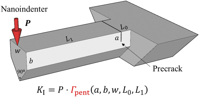
The selected benchmark problem comes from a practical experimental method for measuring fracture toughness (16–19) of brittle isotropic materials (e.g., polycrystalline silicon) by loading a prenotched microcantilever of pentagonal cross-section at its free end, as shown in Fig. 1. The fracture toughness is correlated directly with the critical load at the onset of fracture as well as a set of parameters that define the specimen geometry, $\left\{a,b,w,L_0,L_1\right\}$. The relationship that describes the stress intensity factor, $K_I$, at the crack tip for a given load, $P$, is required. Note that this is essentially a linear elastic boundary value problem involving five independent dimensionless variables:

$$\begin{array}{c}\{\begin{array}{c}\underset{¯}{x}=\left(x_1,x_2,x_3,x_4\right)=\left(\frac{a}{b},\frac{w}{b},\frac{L_0}{b},\frac{L_1}{b}\right)\hspace{1em}\\ y=\frac{K_I}{P{L}_1{a}^{0.5}{b}^{-1}{w}^{-2}}\hspace{1em}\end{array}.\end{array}$$ [1]

The correlation between $y$ and $\underset{¯}{x}$ needs to be extracted (20), so that the ratio of the stress intensity factor to the applied load, $K_I/P={\mathrm{\Gamma }}_{pent}\left(a,b,w,L_0,L_1\right)$, can be obtained.

Fig. 1.

Selected demonstration problem from a common sample to measure fracture toughness at small scales. A prenotched microcantilever with pentagonal cross-section, whose dimensions are $\left\{w,b,a,L_0,L_1\right\}$, is loaded at one end using a nanoindenter. The fracture toughness is directly correlated with the critical load at the onset of fracture as well as the specimen geometry. The relationship, ${\mathrm{\Gamma }}_{pent}$, that describes the stress intensity factor, $K_I$, at the crack tip for a given load, $P$, is required for a valid toughness measurement.

This correlation can be extracted in a data-driven manner and stored as a predictive ML model, enabling broad application of this fracture toughness characterization method. Note that in such tests specimens are typically micromachined by focused ion beams and their dimensions cannot be precisely controlled (16–19). More specifically, the ML solution should provide an accurate output of $y$ for an arbitrary input $\underset{¯}{x}$ in a predefined parameter space, which in the present case is $\mathrm{\Lambda }=\left[0.1,\hspace{0.17em}0.8\right]\times \left[1.0,\hspace{0.17em}3.0\right]\times \left[0.1,\hspace{0.17em}0.4\right]\times \left[2.0,\hspace{0.17em}5.0\right]$, according to the range of microcantilever dimensions used in practice. The dataset for knowledge extraction comprises $\underset{¯}{x}\in \mathrm{\Lambda }$ and its corresponding target value of $y$, i.e., $y_{target}$, from 3D finite element simulations (more details in Data Acquisition from Finite Element Simulations).

The development of such a predictive ML model includes model selection, training, and assessment. To find an appropriate model, the “link” from the four inputs, $\underset{¯}{x}=\left(\frac{a}{b},\frac{w}{b},\frac{L_0}{b},\frac{L_1}{b}\right)$, to the output, $y$, needs to be identified. The following question can be immediately raised: Are all inputs important for establishing such a link? To address this issue, a data-based tool is built to quantify the importance of each input (more details in Quantification of the Feature Importance). With this tool, and by using a small amount of data, the relative error of the target variable, $y$, caused by neglecting its dependence on $x_i$ is found to be at least 63.0%, 52.3%, 19.7%, and 37.2%, respectively. Therefore, all four inputs are indispensable for this problem. A fully connected neural network (NN) with rectified linear activation function (ReLU) is selected, which consists of an input layer with four nodes, two hidden layers with $n_1$ and $n_2$ nodes, and an output layer with a single node, denoted by “$4/n_1/n_2/1$.” A supervised learning problem is then formulated by minimizing the difference between the NN prediction, $y_{pred}$, and the target value from finite element method (FEM), $y_{target}$ (more details in Basic Training Procedure for an ML Model). Informing the model with a training dataset provides a series of different candidates due to the randomness of initialization and training. By testing these candidates with sufficient assessment data their accuracy can be evaluated so that those with an acceptable prediction error can be selected as qualified solutions to the problem.

To provide a broad scope of the correlation between $y$ and $\underset{¯}{x}$, the training data are selected from a uniform grid across the entire parameter space, $\mathrm{\Lambda }$, with each input domain being discretized into $\left(5,\hspace{0.17em}8,\hspace{0.17em}2,\hspace{0.17em}2\right)$ intervals. It is not possible to estimate whether these training data points are enough unless the accuracy of the trained model is correctly assessed. The model accuracy can be defined as the maximum absolute percentage error between the model prediction, $y_{pred}$, and the target value, $y_{target}$ (which corresponds to the worst-case scenario prediction):

$$\begin{array}{c}E=\underset{\underset{¯}{x}\hspace{0.17em}\in \hspace{0.17em}\mathrm{\Lambda }}{\max }\left|\frac{y_{pred}\left(\underset{¯}{x}\right)-y_{target}\left(\underset{¯}{x}\right)}{y_{target}\left(\underset{¯}{x}\right)}\right|\times 100\%.\end{array}$$ [2]

The accuracy assessment is not trivial since it is defined in a continuum parameter space but can only be evaluated in a discrete assessment dataset. Inspired by the idea of mesh convergence in finite element analysis (21), a series of assessment datasets is built by refining the interval of the sampling grid, i.e., $\left\{{\chi }_h^{\left(0\right)},{\chi }_h^{\left(1\right)},{\chi }_h^{\left(2\right)},\dots \right\}$. ${\chi }_h^{\left(0\right)}$ corresponds to a uniform grid with $\left(5,\hspace{0.17em}8,\hspace{0.17em}2,\hspace{0.17em}2\right)$ intervals in each dimension, and ${\chi }_h^{\left(n\right)}$ corresponds to a grid with $\left(5,\hspace{0.17em}8,\hspace{0.17em}2,\hspace{0.17em}2\right)\times 2^n$ intervals. The prediction error of a trained model is evaluated on these datasets, and a nondecreasing sequence of estimates of the model accuracy is obtained, i.e., $\left\{E_h^{\left(0\right)},E_h^{\left(1\right)},E_h^{\left(2\right)},\dots \right\}$, the convergent value of which provides a reliable estimate of model accuracy in the continuous parameter space, i.e., $E=E_h^{\left(\infty \right)}$. If none of the trained models achieves the desired accuracy, a larger training dataset or a more complicated model architecture should be employed. This iterative framework will ultimately provide a qualified predictive model regardless of how the initial grid, ${\chi }_h^{\left(0\right)}$, is selected. Moreover, the fact that the information is not distributed evenly across the uniform grids motivates our active learning study of data collection in An Active Learning Approach to Accuracy Assessment.

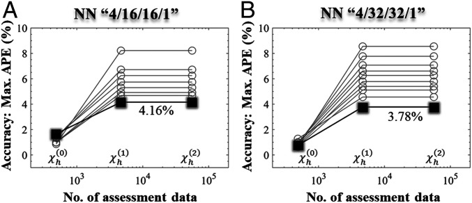
As shown in Fig. 2, different NN structures, “4/16/16/1” and “4/32/32/1,” are selected. The details of the training procedure are described in Basic Training Procedure for an ML Model. It is found that the smallest assessment dataset, ${\chi }_h^{\left(0\right)}$, which is also used for training, cannot provide a correct value of the model accuracy. Most of the trained models can be correctly assessed with ${\chi }_h^{\left(2\right)}$, i.e., a convergent value of the model accuracy is observed with 56,133 data points. Among the well-assessed models, one can choose the appropriate model according to their accuracy. Specifically, using 486 training data and 56,133 assessment data, a predictive model with less than 5.0% relative error can be obtained, which stores the desired knowledge for this problem. It is worth noting that while we have used the four dimensionless variables, $\underset{¯}{x}=\left(\frac{a}{b},\frac{w}{b},\frac{L_0}{b},\frac{L_1}{b}\right)$, as descriptors of the fracture mechanics problem under study, in general more advanced feature encoding methods, e.g., Fourier descriptor (22) or the principal component of the signed distance function (23), can be employed for more complicated geometries. While simple NNs with a few hidden nodes are selected in this work, other approaches, such as the extreme learning machine algorithm with a single-hidden layer feedforward NN (24), may also be employed for this problem.

Fig. 2.

Accuracy assessment of the predictive models is data-demanding. NNs with different structures, (A) “4/16/16/1” and (B) “4/32/32/1,” are selected to extract knowledge from a small dataset, ${\chi }_h^{\left(0\right)}$. The resulting predictive models are assessed with a series of enriched datasets, ${\chi }_h^{\left(1\right)}$ and ${\chi }_h^{\left(2\right)}$. Due to the randomness of initialization and training, these models have different prediction performances. With ${\chi }_h^{\left(1\right)}$ and ${\chi }_h^{\left(2\right)}$, these models exhibit a convergent value of the maximum absolute percentage error (max. APE) between the model prediction and target value. The convergent value provides a reliable estimate of the accuracy of these models. The best predictive models exhibit a relative error of less than 4.16% and 3.78%, respectively, for the two cases.

Thus, a template approach to accuracy assessment in the general framework for extracting a predictive model involves a large amount of data. The total consumption for acquiring 56,133 data is ∼25,000 central processing unit (CPU) hours with the finite element software FEAP (25). Surprisingly, the majority of data usage is allocated to accuracy assessment rather than knowledge extraction.

An Active Learning Approach to Accuracy Assessment.

Data scarcity is a major challenge in building an accurate predictive ML model. The results in Accurate Knowledge Extraction Is Data-Demanding have demonstrated that the model accuracy can be assessed by progressively acquiring data in a brute-force manner, i.e., by sampling the full parameter space with a uniform and refining interval. However, such systematic sampling can be inefficient due to noninformative data. Active learning and design-of-experiment approaches alleviate the need for large datasets by selecting the most informative data (26–28). Thus, the goal is to identify points where the model exhibits the largest prediction error without knowing the target values (as defined in Eq. 1) beforehand or requiring any prior physical information associated with the problem.

Inspired by recent developments in computer science (26, 27, 29), we employ the so-called query-by-committee algorithm. Here, a committee of mutually independent models, $C=\left\{{\widehat{y}}^{\left(1\right)},{\widehat{y}}^{\left(2\right)},\dots ,{\widehat{y}}^{\left(N_c\right)}\right\}$, is established, which shows consistent predictive values with the currently available data. The pointwise prediction error of the committee is defined as

$$\begin{array}{c}\epsilon \left(\underset{¯}{x}\right)=\underset{i=\mathrm{1,2},\dots ,\hspace{0.17em}{N}_c}{\max }\left|\frac{{\widehat{y}}^{\left(i\right)}\left(\underset{¯}{x}\right)-y_{target}\left(\underset{¯}{x}\right)}{y_{target}\left(\underset{¯}{x}\right)}\right|.\end{array}$$ [3a]

Based on the premise that the committee’s predictions at each point in the parameter space follow an unbiased distribution, the average prediction serves as an optimal alternative to the target value, i.e., $\overline{y}=\frac{1}{N_c}{\displaystyle \sum _i{\widehat{y}}^{\left(i\right)}\left(\underset{¯}{x}\right)}$ and $\underset{N_c\to \infty }{\lim }\overline{y}=y_{target}$. On this basis, the pointwise prediction error of the committee, $\epsilon \left(\underset{¯}{x}\right)$, can be approximated by

$$\begin{array}{c}\stackrel{\sim }{\epsilon }\left(\underset{¯}{x}\right)=\underset{i}{\max }\left|\frac{{\widehat{y}}^{\left(i\right)}\left(\underset{¯}{x}\right)-\overline{y}\left(\underset{¯}{x}\right)}{\overline{y}\left(\underset{¯}{x}\right)}\right|.\end{array}$$ [3b]

Since the number of committee members, $N_c$, is limited by practical considerations, the value of $\epsilon \left(\underset{¯}{x}\right)$ could be slightly different from $\stackrel{\sim }{\epsilon }\left(\underset{¯}{x}\right)$ . However, such disturbance barely affects the effort to detect locations where $\epsilon \left(\underset{¯}{x}\right)$ attains local maximum values from $\stackrel{\sim }{\epsilon }\left(\underset{¯}{x}\right)$. In other words, the maximum values of $\stackrel{\sim }{\epsilon }\left(\underset{¯}{x}\right)$ and $\epsilon \left(\underset{¯}{x}\right)$ in a local patch, $\mathrm{\Lambda }\prime$, of the parameter space, $\mathrm{\Lambda }$, are found to be nearly colocalized:

$$\begin{array}{c}\underset{\underset{¯}{x}\hspace{0.17em}\in \hspace{0.17em}{\mathrm{\Lambda }}^{\prime }}{\text{arg}\hspace{0.17em}\text{max}}\epsilon \left(\underset{¯}{x}\right)\approx \underset{\underset{¯}{x}\hspace{0.17em}\in \hspace{0.17em}{\mathrm{\Lambda }}^{\prime }}{\text{arg}\hspace{0.17em}\text{max}}\stackrel{\sim }{\epsilon }\left(\underset{¯}{x}\right).\end{array}$$ [4]

The evaluation of $\stackrel{\sim }{\epsilon }\left(\underset{¯}{x}\right)$ would guide us to points where the committee shows the largest prediction error. Acquiring the target values at these points allows an accuracy assessment of the committee and provides crucial data for improving the committee’s overall accuracy. Note that the purpose of our committee setup for accuracy assessment in active learning is different from that of the ensemble method in ML (30), which aims to make a definitive prediction based on a weighted sum of each member’s prediction.

Accordingly, an iterative framework for collecting data is formulated (discussed in detail in Committee-Based Active Learning Approach). During each iteration, 20,000 NNs of the same structure (“4/32/32/1”) are trained with all the available data. More than 60% of the NN models make predictions with a relative error of less than 1.0% at these data points. These models are then enrolled into the committee. The points with the largest values of $\stackrel{\sim }{\epsilon }\left(\underset{¯}{x}\right)$ are found throughout the parameter space, and the target values at these points are acquired from simulations so that the maximum prediction error of the committee, $E_{\text{c}}$, can be assessed. The newly collected data are added to the current dataset and utilized for the next iteration. The iteration ends when the desired accuracy is achieved.

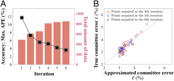
This active learning approach significantly improves the efficiency of data usage for accuracy assessment and knowledge extraction, as shown in Fig. 3. After five iterations, using 486 initial and 362 newly collected data, a committee of NNs with less than 5.0% relative error is established. Each committee member is a qualified and well-assessed ML model that provides precise predictions with less than 5.0% relative error. To verify the assumption that $\epsilon \left(\underset{¯}{x}\right)$ and $\stackrel{\sim }{\epsilon }\left(\underset{¯}{x}\right)$ are colocalized (as described in Eq. 4), their behaviors for newly selected points in each iteration are evaluated. As expected, the point with a larger value of $\stackrel{\sim }{\epsilon }\left(\underset{¯}{x}\right)$ usually exhibits a larger value of $\epsilon \left(\underset{¯}{x}\right)$, especially when $\stackrel{\sim }{\epsilon }\left(\underset{¯}{x}\right)\ge 4.0\%$.

Fig. 3.

The iterative active learning framework for extracting knowledge with metrics. (A) The iteration is initialized with 486 data points, which are uniformly dispersed in the parameter space. Through training 20,000 NNs of the same structure (“4/32/32/1”), a committee of more than 12,000 models is established. The committee’s accuracy is estimated to be less than 12% relative error by acquiring selective data from simulations. The newly collected data are utilized in the next iteration. After five iterations, 362 new data points are collected, and a group of NNs with less than 5.0% relative error is obtained. (B) The premise that $\epsilon \left(\underset{¯}{x}\right)$ and $\stackrel{\sim }{\epsilon }\left(\underset{¯}{x}\right)$ are colocalized (as described Eq. 4) is verified with the newly selected points in each iteration. As expected, $\stackrel{\sim }{\epsilon }\left(\underset{¯}{x}\right)$ is a good approximation to $\epsilon \left(\underset{¯}{x}\right)$.

Data-Driven Knowledge Transfer.

The results in Accurate Knowledge Extraction Is Data-Demanding and An Active Learning Approach to Accuracy Assessment have demonstrated that the desired knowledge can be extracted from simulation data without any prior knowledge of the system, as most important physical information is already contained in the dataset. Naturally, it can be expected that the incorporation of physical knowledge of the system may have a significant impact on creating the predictive model. Some prior attempts used physics-informed ML models, i.e., NNs coupled with governing equations, for capturing the physical correlation between inputs and outputs (26, 31). However, there is no governing equation that can be theoretically derived for the fracture problem under consideration. Instead, an existing ML model that deals with a similar but simpler problem might be more likely to provide useful knowledge. This follows the idea of transfer learning, i.e., the knowledge gained while learning to solve one problem can be transferred to help solve another.

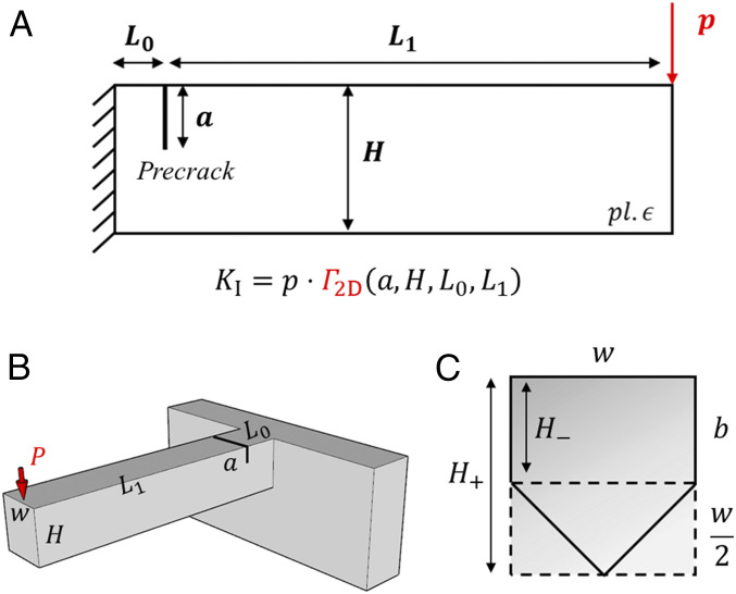
Here, it is interesting to note that the fracture of a notched cantilever with pentagonal cross-section is similar to that of a 2D notched cantilever under a line force $p$, as shown in Fig. 4A. The knowledge gained from solving this 2D problem, which is much easier compared to the 3D problem, can be stored as an auxiliary ML solution, i.e., $K_I=p\cdot {\mathrm{\Gamma }}_{2D}\left(a,H,L_0,L_1\right)$. The establishment of ${\mathrm{\Gamma }}_{2D}$ is detailed in SI Appendix.

Fig. 4.

The pentagonal cross-section cantilever shares a similar feature of fracture with a 2D notched cantilever. (A) A 2D notched cantilever, whose dimensions are $\left\{a,H,L_0,L_1\right\}$, is loaded at its free end by a line force, $p$. The established solution to this problem, ${\mathrm{\Gamma }}_{2D}$, describes the stress intensity factor at the crack, $K_I$, for a given $p$. (B)${\mathrm{\Gamma }}_{2D}$ can also be used to predict the stress intensity factor for a rectangular cross-section cantilever (width $w$ and height $H$) under an external load, $P$. (C) The pentagonal cross-section falls in between two corresponding rectangular cross-sections: One is contained within the pentagon and the other itself contains the pentagon. It is postulated that the solution for the notched cantilever with pentagonal cross-section, ${\mathrm{\Gamma }}_{pent}$, is implicitly connected to its rectangular cross-section counterparts (described by ${\mathrm{\Gamma }}_{2D}$).

The transfer of the auxiliary solution relies on mining the connection between ${\mathrm{\Gamma }}_{pent}$ and ${\mathrm{\Gamma }}_{2D}$. Discovering this connection is not a trivial task as it requires advanced data analysis. Note that ${\mathrm{\Gamma }}_{2D}$ has the capability of predicting the stress intensity factor for a rectangular cross-section cantilever (width $w$ and height $H$), i.e., $K_I/P=w^{-1}\cdot {\mathrm{\Gamma }}_{2D}\left(a,H,L_0,L_1\right)$, as shown in Fig. 4B. By comparing the beam compliance of the pentagonal cross-section cantilever and the rectangular cross-section cantilevers (width $w$ and height $H_{\pm }=b+\frac{w}{4}\pm \frac{w}{4}$), an intuitive relation can be formed:

$$\begin{array}{c}{\mathrm{\Gamma }}^n=\alpha {\mathrm{\Gamma }}_{+}^n+\left(1-\alpha \right){\mathrm{\Gamma }}_{-}^n,\end{array}$$ [5a]

where $\mathrm{\Gamma }={\mathrm{\Gamma }}_{pent}\left(a,b,w,L_0,L_1\right)$ and ${\mathrm{\Gamma }}_{\pm }=w^{-1}\cdot {\mathrm{\Gamma }}_{2D}\left(a,H_{\pm },L_0,L_1\right)$. For an arbitrary configuration $\left\{a,b,w,L_0,L_1\right\}$, the values of ${\mathrm{\Gamma }}_{\pm }$ are known beforehand. However, the interpolation coefficient, $\alpha \in \left(0,\hspace{0.17em}1\right)$, has yet to be determined. Through dimensional analysis, $\alpha$ should be a bounded function of four independent dimensionless variables, $\underset{¯}{x}=\left(x_1,x_2,x_3,x_4\right)=\left(\frac{a}{b},\frac{w}{b},\frac{L_0}{b},\frac{L_1}{b}\right)$, and one tuning parameter, $n$:

$$\begin{array}{c}\alpha ={\alpha }_n=\alpha \left(x_1,x_2,x_3,x_4;n\right).\end{array}$$ [5b]

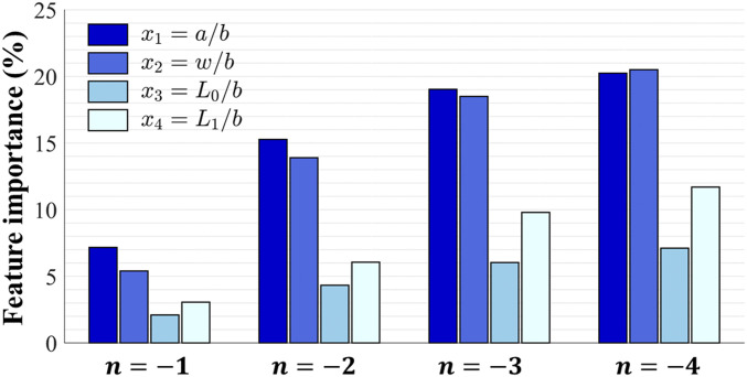
The importance of $x_i$ to $\alpha$ can be identified conveniently from 16 different configurations of $\underset{¯}{x}$ (more details in Quantification of the Feature Importance), which estimates the possible deviation of $\mathrm{\Gamma }$ in Eq. 5 if the dependence of $\alpha$ on $x_i$ is neglected. The additional flexibility factor, $n$, is intentionally introduced to tune the importance of $x_i$, as shown in Fig. 5. Surprisingly, an optimal value of $n=-1$ is found, in which case the importance of $\underset{¯}{x}$, especially $x_3$ and $x_4$, are minimized. This observation provides valuable insights into the undiscovered connection between ${\mathrm{\Gamma }}_{pent}$ and ${\mathrm{\Gamma }}_{2D}$. More specifically, the dependence of $\alpha$ on $x_{\mathrm{3,4}}$ and even $x_{\mathrm{1,2}}$ can be reduced if the resulting deviation of $\mathrm{\Gamma }$ in Eq. 5 is within tolerance.

Fig. 5.

Identifying and tunning the importance of $x_i$ to the prediction of ${\mathrm{\Gamma }}_{pent}$. The (feature) importance of $x_i$ to $\alpha$ can be identified from 16 different configurations of $\underset{¯}{x}$, which can be further tuned by varying the additional flexibility factor, $n$ (Eq. 5). Interestingly, the optimal value of $n=-1$ is found to minimize the importance of $\underset{¯}{x}$, especially $x_3$ and $x_4$. This observation provides valuable insights into the choice of $\alpha$, as well as the establishment of the connection between ${\mathrm{\Gamma }}_{pent}$ and ${\mathrm{\Gamma }}_{2D}$.

The ideal scenario is that $\alpha$ can be replaced with a constant, e.g., $\overline{\alpha }=0.5452$, which is acquired from the center of the parameter space. As a result, a reduced expression of $\mathrm{\Gamma }$ is obtained:

$$\begin{array}{c}\overline{\mathrm{\Gamma }}=\frac{1}{\overline{\alpha }{\mathrm{\Gamma }}_{+}^{-1}+\left(1-\overline{\alpha }\right){\mathrm{\Gamma }}_{-}^{-1}},\hspace{0.17em}\hspace{0.17em}\overline{\alpha }=\mathrm{0.5452.}\end{array}$$ [6]

To validate this simplification, the relative error between $\overline{\mathrm{\Gamma }}$ and its target value from finite element simulations needs to be evaluated. By sampling the parameter space with a uniform and refining interval, the relative error is estimated, in a reliable manner, to be less than 7% with 625 data points. This marginal deviation suggests a successful practice of knowledge transfer, i.e., the knowledge of how $\overline{\mathrm{\Gamma }}$ depends on $\underset{¯}{x}$ is almost fully inherited from the auxiliary solution, ${\mathrm{\Gamma }}_{2D}$.

The relative error of $\overline{\mathrm{\Gamma }}$ in Eq. 6 can be narrowed by incorporating the dependence of $\alpha$ on $x_1$ and $x_2$, i.e., by replacing $\overline{\alpha }$ with $\widehat{\alpha }\left(x_1,x_2\right)$. To establish this function, an intermediate value of $x_{\mathrm{3,4}}=x_{\mathrm{3,4}}^{\ast }=\left(0.25,\hspace{0.17em}3.5\right)$ is chosen from the center of the parameter space. Also, for arbitrary $x_{\mathrm{1,2}}$ combined with the selected $x_{\mathrm{3,4}}^{\ast }$, a unique value of $\alpha$ can be determined by Eq. 5, which provides a one-to-one mapping, i.e., $\widehat{\alpha }=\widehat{\alpha }\left(x_1,x_2\right)$. Thus, a new reduced expression of $\mathrm{\Gamma }$ is proposed:

$$\begin{array}{c}\widehat{\mathrm{\Gamma }}=\frac{1}{\widehat{\alpha }{\mathrm{\Gamma }}_{+}^{-1}+\left(1-\widehat{\alpha }\right){\mathrm{\Gamma }}_{-}^{-1}},\hspace{0.17em}\hspace{0.17em}\widehat{\alpha }=\widehat{\alpha }\left(x_1,x_2\right).\end{array}$$ [7]

Similarly, with 625 data points, the relative error between $\widehat{\mathrm{\Gamma }}$ and its target value is estimated to be less than 3%. Compared with Eq. 6, the dependence of ${\mathrm{\Gamma }}_{2D}$ on $x_{\mathrm{3,4}}$ (instead of all variables) is transferred, and the relative error of $\widehat{\mathrm{\Gamma }}$ is narrowed. Interestingly, a balance between simplicity and accuracy is achieved in Eq. 7 with this selective knowledge transfer.

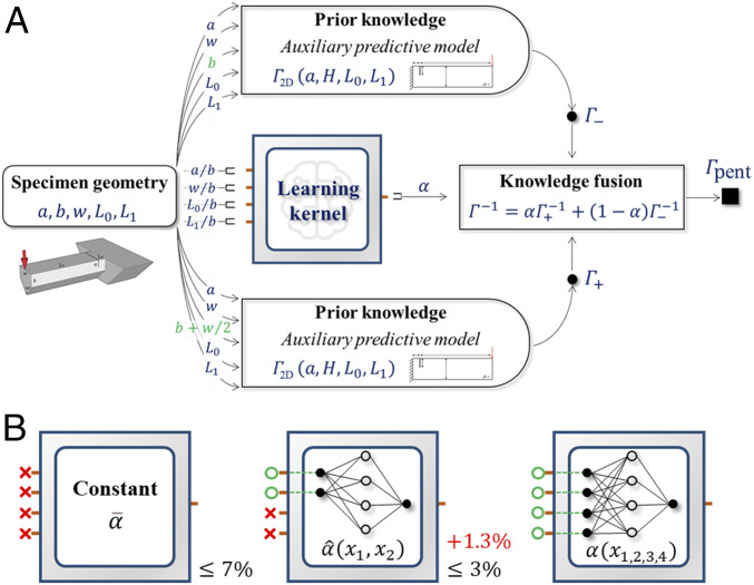
Therefore, a practical protocol of knowledge transfer from ${\mathrm{\Gamma }}_{2D}$ to ${\mathrm{\Gamma }}_{\text{pent}}$ is formulated (Eqs. 6 and 7), in which the simplification of $\alpha$ to $\overline{\alpha }$ and $\widehat{\alpha }$ is crucial. On this basis, a hierarchical framework for predicting ${\mathrm{\Gamma }}_{\text{pent}}$ is established, as shown in Fig. 6. The dependence of $\alpha$ on $\underset{¯}{x}$ is represented by a switchable kernel in this framework, which can have multiple versions, i.e., $\overline{\alpha }$ and $\widehat{\alpha }$. Note that these two versions feature different levels of simplification and error tolerance. If the constant $\overline{\alpha }$ is selected, this framework predicts ${\mathrm{\Gamma }}_{\text{pent}}$with less than 7% relative error. If $\widehat{\alpha }$ is selected, this framework has the capability of predicting ${\mathrm{\Gamma }}_{\text{pent}}$ with less than 3% relative error. Note that the knowledge of $\widehat{\alpha }$ needs to be extracted from a set of discrete data, which causes additional error in the prediction of ${\mathrm{\Gamma }}_{\text{pent}}$. For example, a simple fully connected NN with two nodes in the input layer, four nodes in the hidden layer, and a single node in the output layer, denoted by “2/4/1,” can be employed for learning $\widehat{\alpha }\left(x_1,x_2\right)$. A small dataset ${\chi }_{\text{reduced}}^{\left(0\right)}$ is acquired from a uniform grid across the reduced parameter space, ${\mathrm{\Lambda }}_{\text{reduced}}=\left[0.1,\hspace{0.17em}0.8\right]\times \left[1.0,\hspace{0.17em}3.0\right]$, with each input domain being discretized into $\left(4,\hspace{0.17em}4\right)$ intervals. By refining the interval of the sampling grid, two enriched datasets, ${\chi }_{\text{reduced}}^{\left(1\right)}$ and ${\chi }_{\text{reduced}}^{\left(2\right)}$, can be obtained, corresponding to grids with $\left(8,\hspace{0.17em}8\right)$ and $\left(16,\hspace{0.17em}16\right)$ intervals. The NN is informed by ${\chi }_{\text{reduced}}^{\left(0\right)}$ (more details in Basic Training Procedure for an ML Model) and assessed on ${\chi }_{\text{reduced}}^{\left(1\right)}$ and ${\chi }_{\text{reduced}}^{\left(2\right)}$. It is found that an additional error of 1.3% for predicting ${\mathrm{\Gamma }}_{\text{pent}}$ arises when $\widehat{\alpha }$ is approximated by the trained NN.

Fig. 6.

The hierarchical framework for predicting ${\mathrm{\Gamma }}_{\text{pent}}$ based on knowledge transfer. (A) The predictive framework utilizes the well-established auxiliary solution, ${\mathrm{\Gamma }}_{2D}$, and the discovered connection to predict ${\mathrm{\Gamma }}_{\text{pent}}$. The switchable kernel in this framework, which concretizes the dependence of $\alpha$ on $\underset{¯}{x}$, can have multiple versions, i.e., $\overline{\alpha }$ and $\widehat{\alpha }$ (Eqs. 6 and 7). (B) These two versions feature different levels of error tolerance, less than 7% and 3% relative error for $\overline{\alpha }$ and $\widehat{\alpha }$, respectively. Note that the original form of $\alpha$ in Eq. 5 shows the best approximation capability but does not provide a solid connection between ${\mathrm{\Gamma }}_{2D}$ and ${\mathrm{\Gamma }}_{\text{pent}}$. The second kernel, $\widehat{\alpha }$, is established with a simple fully connected NN (“2/4/1”), which adds 1.3% relative error.

The above example of successful knowledge transfer provides a unique perspective on how to solve a linear elastic fracture mechanics problem in a data-driven manner. Instead of directly extracting the solution from data (as discussed in Accurate Knowledge Extraction Is Data-Demanding and An Active Learning Approach to Accuracy Assessment), finding its relevance to a resolved auxiliary problem through careful data analysis can provide useful insights. Once the connection between these problems is established, the solution can be built on the existing knowledge from the auxiliary problem, rather than from scratch. This may substantially shorten the time and reduce the cost for solving a complex problem. Our selected benchmark problem showcases the capabilities of data-driven knowledge transfer in fracture mechanics. A framework (Fig. 6A) is designed based on the discovered connection (Eqs. 6 and 7) between the unsolved problem of a pentagonal cross-section cantilever (Fig. 1) and the resolved 2D counterpart (Fig. 4). The replaceable kernel can switch between $\overline{\alpha }$ and $\widehat{\alpha }$ (Fig. 6B), which provides two reliable predictive models with less than 7% and 5% relative error, respectively. Interestingly, most of the data, i.e., 625 data points, are used to discover the hidden connection while only a small amount of data are required for extracting the switchable kernel, i.e., 1 point for $\overline{\alpha }$ or 289 points for $\widehat{\alpha }$. This practice offers a state-of-the-art combination of data-driven knowledge transfer and knowledge extraction in fracture mechanics, which turns out to be data-efficient.

Discussion

Importance of Knowledge Accuracy.

In this work, both knowledge extraction and knowledge transfer are demonstrated to be effective approaches in data-driven fracture mechanics. The importance of knowledge accuracy for making predictions is highlighted. Inaccuracies in knowledge mainly arise from either unreliable data sources or limited approximation capabilities of the selected ML models. The first issue can be resolved through proper data acquisition, e.g., high-resolution FEM. The latter is inevitable, making an estimation of the resulting error necessary. However, reliable accuracy assessment is data-demanding and challenging as all possible configurations of the problem need to be explored. To enable accuracy assessment in a data-limited regime, a tailored active learning approach is proposed. This approach relies on establishing an unbiased and independent committee, i.e., a large assembly of well-informed ML models. The average of the committee members’ predictions provides an optimal alternative to the target value, which is essential for locating the configurations where the committee has the largest prediction error. By acquiring the target values for these high-risk configurations, the upper bound of each committee member’s prediction error is determined, causing all the models in the committee to be well-assessed. It is important to collect enough committee members (∼10 times larger than the degrees of freedom in the ML model) to guarantee that the average prediction from the committee is a valid approximation to the target value, which sets the basis for accuracy assessment. On the other hand, the newly acquired data during this process are expected to be most useful in improving the overall accuracy of the committee. This forms an iterative framework for learning and assessment, which ultimately provides a group of accurate and well-assessed ML models using a small amount of data.

Unraveling Hidden Connections between Related Problems Enables Knowledge Transfer.

The success of knowledge transfer in data-driven fracture mechanics is expected to benefit from advanced data analytics, as well as human intelligence and well-established domain knowledge. First, it is essential to find an appropriate auxiliary problem that is relevant and resolved, with the input of researchers’ experience and intuition. Second, the underlying connection between the auxiliary problem and the problem under consideration needs to be recovered from a limited amount of data via intelligent data analysis and knowledge extraction. Finally, the discovered connection can be incorporated into a hybrid framework, which transfers the prior knowledge to the current problem. The combination of knowledge transfer and extraction not only offers engaging opportunities for further exploration of data-driven fracture mechanics but also poses challenges of enhancing the versatility and accuracy of the extracted knowledge.

The Elegance and Versatility of the Established Connection.

Dirac wrote, “A physical law must possess mathematical beauty.” The established connection (in two versions, Eqs. 6 and 7) can be revisited under this principle. Note that both versions are derived from Eq. 5, in which $\mathrm{\Gamma }$ is expressed as a weighted generalized mean of ${\mathrm{\Gamma }}_{\pm }$ with a coefficient $\alpha$ and exponent $n$. Determining $\alpha$ and $n$ in Eqs. 6 and 7 provides a physical connection between $\mathrm{\Gamma }$ and ${\mathrm{\Gamma }}_{\pm }$. The discovery of both the integer exponent, $n=1$, and the weak dependance of $\alpha$ on various configurations significantly simplifies the connection. Interestingly, by assuming $\alpha =1/2$, $\mathrm{\Gamma }$ takes a more concise form, i.e., the harmonic mean of ${\mathrm{\Gamma }}_{\pm }$:

$$\begin{array}{c}\overline{\overline{\mathrm{\Gamma }}}=\frac{2}{{\mathrm{\Gamma }}_{+}^{-1}+{\mathrm{\Gamma }}_{-}^{-1}}.\end{array}$$ [8]

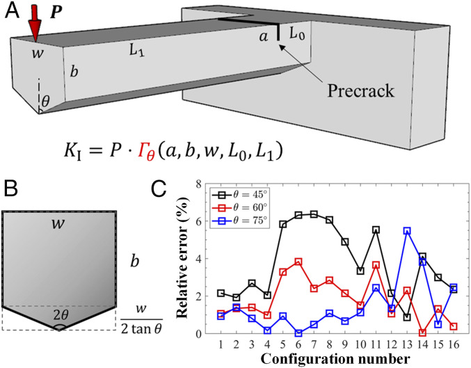
The deviation of the connection from the acquired data might be an artifact caused by either numerical errors from simulations or by the inaccuracy of the prior knowledge. It is anticipated that the recovered connection (Eq. 8) can be applied to a series of new fracture mechanics problems, which are formulated by relaxing the constraint on the bottom angle, $2\theta$, of the pentagonal cross-section (Fig. 7 A and B). With ${\mathrm{\Gamma }}_{\pm }=w^{-1}\cdot {\mathrm{\Gamma }}_{2D}\left(a,b+\frac{w}{4\tan \theta }\pm \frac{w}{4\tan \theta },L_0,L_1\right)$ being modified accordingly, the prediction of $\mathrm{\Gamma }$ by Eq. 8 is consistent with the simulation results in Fig. 7C and Table 1. It is worth pointing out that other methods such as symbolic regression (32) could potentially enable such knowledge transfer as well. For example, the mathematically concise connection (Eq. 8) may also be uncovered using purely data-driven symbolic regression. In comparison, our present study suggests that combining domain knowledge and data analytics can make the knowledge transfer more interpretable.

Fig. 7.

Application of the recovered connection to a series of new fracture mechanics problems. (A) A prenotched microcantilever, with a modified pentagonal cross-section, is loaded at one end. It is desired to determine the ratio of the stress intensity factor at the crack tip, to the external load, i.e., ${\mathrm{\Gamma }}_{\theta }=K_I/P$. (B) The new problems are formed based on the original one (in Fig. 1) by relaxing the constraint on the bottom angle, $2\theta$, of the pentagonal cross-section. Note that the modified pentagonal cross-section falls in between two rectangular cross-sections. (C) The recovered connection (Eq. 8) is demonstrated to be applicable to these new problems, with ${\mathrm{\Gamma }}_{\pm }$ being modified accordingly. The difference between the prediction by Eq. 8 and the simulation results is less than 10% for different angles, $\theta$, and different configurations, as listed in Table 1.

Table 1.

Comparison between the recovered connection and finite element simulations

Configurationno.	$\mathit{a}/\mathit{b}$	$w/b$	${\mathit{L}}_0/\mathit{b}$	${\mathit{L}}_1/\mathit{b}$	Relative error*
					θ = 45°,%	θ = 60°,%	θ = 75°,%
1	0.10	1.00	0.10	2.00	2.15	1.06	0.93
2	0.10	1.00	0.10	5.00	1.92	1.34	1.40
3	0.10	1.00	0.40	2.00	2.69	1.40	0.81
4	0.10	1.00	0.40	5.00	2.05	0.98	0.17
5	0.10	3.00	0.10	2.00	5.83	3.28	0.93
6	0.10	3.00	0.10	5.00	6.32	3.84	0.02
7	0.10	3.00	0.40	2.00	6.36	2.40	0.48
8	0.10	3.00	0.40	5.00	6.06	2.84	1.08
9	0.80	1.00	0.10	2.00	4.89	2.15	0.66
10	0.80	1.00	0.10	5.00	3.34	1.51	1.12
11	0.80	1.00	0.40	2.00	5.54	3.66	2.44
12	0.80	1.00	0.40	5.00	2.15	1.06	1.35
13	0.80	3.00	0.10	2.00	0.87	2.30	5.48
14	0.80	3.00	0.10	5.00	4.11	0.04	3.82
15	0.80	3.00	0.40	2.00	2.99	1.32	0.49
16	0.80	3.00	0.40	5.00	2.35	0.38	2.47

^*The relative error is defined as $\left|\left(\overline{\overline{\mathrm{\Gamma }}}-{\mathrm{\Gamma }}_{\text{target}}\right)/{\mathrm{\Gamma }}_{\text{target}}\right|\times 100\%$, where ${\mathrm{\Gamma }}_{\text{target}}$ is acquired from finite element simulations.

The Principle behind the Established Connections.

Although the recovered connection (Eq. 8) arises from data analysis, rather than an interpretable physical theory, it would be interesting to investigate its physical origin and insights. First, the discovery of the connection is enlightened by the 2D nature of the stress field near the straight crack front in the cantilevers (Figs. 1, 4, and 7). Second, these cantilevers differ by additional 3D geometric feature of the boundary (Figs. 1 and 7), while maintaining the 2D feature of the crack front. In short, these cantilevers are characterized by an identical 2D feature, e.g., $K_I$, although they exhibit differences in geometry. The geometric difference affects $K_I$ when an external load, $P$, is applied. Therefore, the shared feature, $K_I$, in the pentagonal cross-section cantilever may be recovered from its 2D counterparts, in a similar manner that the geometric complexity can be related to a 2D cantilever (or a rectangular cross-section cantilever). The area of a pentagon is the average of that of two rectangles (Fig. 4C), and the ratio of $K_I$ to $P$ in the pentagonal cross-section cantilever can be estimated as a generalized mean of $K_I/P$ in the rectangular (2D) counterparts (Eq. 8). Overall, the above discussion rationalizes the principle behind the discovered connection, for which a rigorous theoretical derivation is not feasible. If the geometric complexity of a fracture problem does not severely distort its similarity to a set of resolved problems (e.g., similar notched cantilevers and same fracture mode in this work), then their intrinsic connection may be recovered using a weighted generalized mean of solutions to the latter.

Universality of the Guiding Principle for Knowledge Transfer.

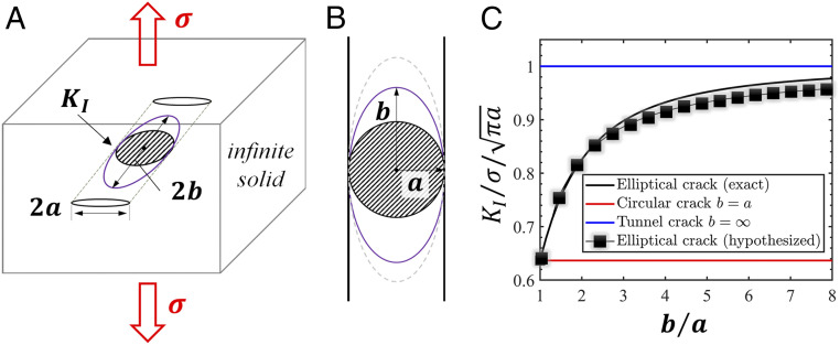
From a more general perspective, this principle can be applied to several different scenarios. 1) Different loading modes, e.g., pure bending and axial tension, can be applied to the cantilevers, while keeping the 2D feature of the fracture mechanics problem. Based on this, the following hypothesis is formed: The ratio of $K_I$ to the magnitude of the remote load in the pentagonal cross-section cantilever can be approximated by the generalized mean of its 2D (rectangular) counterparts. 2) Consider a flat elliptical crack (with major axis $b$ and minor axis $a$) embedded in an infinite solid subject to uniform far-field tension, $\sigma$, in the normal direction of the crack plane (as shown in Fig. 8). Although the stress intensity factor is not uniform along the crack front, its maximum, $K_{I,\left(a,b\right)}$, is located at the minor axis vertices. Note that varying $b$ results in a series of ellipses that are tangent to each other at their minor axis vertices including two special cases, a circular crack $\left(b=a\right)$ and a tunnel crack with a straight front $\left(b=\infty \right)$. All these ellipses have the same direction of crack propagation at the minor axis vertices, which suggests $K_{I,\left(a,b\right)}$, $K_{I,\left(a,b=a\right)}$ and $K_{I,\left(a,b=\infty \right)}$ are connected. Their geometric difference can be quantified by the finite number, $b^{-n_1}$, thus the elliptical crack can be approximated by a weighted generalized mean of the tunnel crack and circular crack, with an interpolation coefficient, $\alpha ={\left(b/a\right)}^{-n_1}$. On this basis, the connection between $K_{I,\left(a,b\right)}$, $K_{I,\left(a,b=a\right)}$ and $K_{I,\left(a,b=\infty \right)}$ can be postulated as

$$\begin{array}{c}{K}_{I,\left(a,b\right)}^{n_2}=\left(1-\alpha \right)K_{I,\left(a,\infty \right)}^{n_2}+\alpha K_{I,\left(a,a\right)}^{n_2},\hspace{0.17em}\hspace{0.17em}\alpha ={\left(b/a\right)}^{-n_1}.\end{array}$$ [9]

Similar connection with $n_1=\hspace{0.17em}{n}_2=1$ has been proposed from a different perspective in ref. 33. Since the exact solutions to the internal circular crack, tunnel crack, and elliptical crack are all well-established (33, 34), this hypothesis (Eq. 9) can be readily examined. It is found, with $n_1=\hspace{0.17em}1$ and $n_2=3/2$, the deviation of $K_{I,\left(a,b\right)}$ between the hypothesized solution (Eq. 9) and the exact solution is less than 5%, as shown in Fig. 8C. Therefore, the principle behind these established connections is demonstrated to be universal and provides a unique perspective on how to discover hidden connections and enable knowledge transfer between problems in fracture mechanics.

Fig. 8.

Demonstration of the principle of knowledge transfer for an elliptical crack. (A) Consider an internal elliptical crack (with major axis $b$ and minor axis $a$) in an infinite solid subject to uniform far-field tension, $\sigma$, normal to the crack plane. For the sake of demonstration, it is desired to determine the stress intensity factor at the minor axis vertices, $K_{I,\left(a,b\right)}$. (B) The circular crack $\left(b=a\right)$ and tunnel crack $\left(b=\infty \right)$ are two special cases of the elliptical crack and have the same direction of crack propagation at the minor axis vertices. Based on the guiding principle (discussed in The Principle behind the Established Connections and Universality of the Guiding Principle for Knowledge Transfer), $K_{I,\left(a,b\right)}$, $K_{I,\left(a,b=a\right)}$ and $K_{I,\left(a,b=\infty \right)}$ should be connected. (C) With the exact solutions to the internal circular crack, tunnel crack, and elliptical crack, the hypothesized connection (Eq. 9) is validated. The difference between the hypothesized solution and the exact solution is less than 5% over a broad range of $b/a$.

Methods

Data Acquisition from Finite Element Simulations.

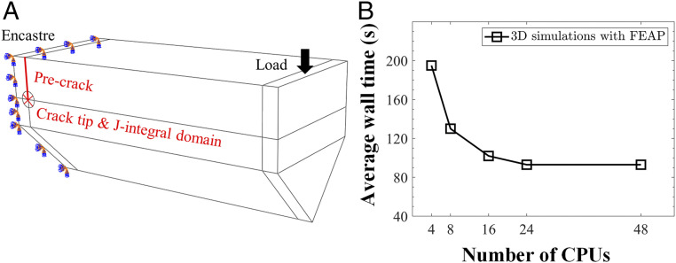
The stress intensity factor, $K_I$, at the crack tip can be evaluated from domain J-integral (35–37) and 3D finite element simulations for the cantilevers with pentagonal cross-section. As shown in Fig. 9, an encastré boundary condition is applied to the fixed end of the cantilever and a displacement-controlled boundary condition to the free end. More than 10,000 full integration elements (C3D20) are employed with refined mesh near the crack tip. The simulations are performed through a user-defined subroutine in the finite element software FEAP (25) or the built-in function in ABAQUS (38). The average wall time for each simulation was ∼100 s when running in parallel on 16 CPUs with FEAP.

Fig. 9.

Data acquisition from FEM simulations. (A) The domain J-integral method is used to evaluate the stress intensity factor at the crack tip. An encastré boundary condition is applied to the fixed end of the cantilever and a displacement-controlled boundary condition to the free end. (B) The computational time of the 3D simulation can be reduced by parallel computing. A typical simulation takes ∼100 s when running in parallel on 16 CPUs with FEAP.

Quantification of the Feature Importance.

The quantification of the importance of inputs (i.e., features) to the prediction of the target output provides valuable insights into the problem. The complexity of the problem can be reduced by neglecting unimportant features. Only relevant features are selected as inputs for the ML model. This also impacts the acquisition of data as the dataset size will shrink with a reduced number of features. Therefore, it is necessary to identify the feature importance of inputs, i.e., $\underset{¯}{x}=\left(x_1,x_2,x_3,x_4\right)$ in our selected problem.

Most of the current methods to evaluate the feature importance rely on the establishment of a predictive model which can tell how sensitive the prediction is to the model inputs (39). These approaches require a large amount of data and appropriate choice of models. Therefore, a simple technique, which only requires a small amount of data and no predictive models, is developed.

To study the dependence of $y$ on $\underset{¯}{x}$ in Eq. 1, a small set of data points are selected from a uniform grid across the entire parameter space, i.e., ${\chi }_{FI}=\left\{x_1^{\left(1\right)},x_1^{\left(2\right)},\dots ,x_1^{\left(N_1\right)}\right\}\times \left\{x_2^{\left(1\right)},x_2^{\left(2\right)},\dots ,x_2^{\left(N_2\right)}\right\}\times \left\{x_3^{\left(1\right)},x_3^{\left(2\right)},\dots ,x_3^{\left(N_3\right)}\right\}\times \left\{x_4^{\left(1\right)},x_4^{\left(2\right)},\dots ,x_4^{\left(N_4\right)}\right\}$. At each point $\underset{¯}{x}=\left(x_1^{\left(i\right)},x_2^{\left(j\right)},x_3^{\left(k\right)},x_4^{\left(l\right)}\right)\in {\chi }_{FI}$, a target value of $y=y^{\left(i,j,k,l\right)}$ can be obtained from simulations. If $y$ is independent of $x_1$, $y^{\left(i_1,j,k,l\right)}=y^{\left(i_2,j,k,l\right)}$ holds for arbitrary $\left(j,k,l\right)$. Otherwise, these values differ greatly. Therefore, the difference among these target values quantifies the feature importance of $x_1$:

$$\begin{array}{c}F{I}_1=\underset{i_1,i_2,j,k,l}{\max }\left|\frac{y^{\left(i_1,j,k,l\right)}-y^{\left(i_2,j,k,l\right)}}{y^{\left(i_2,j,k,l\right)}}\right|.\end{array}$$ [10]

As $N_i$ increases, this is equivalent to the relative error of $y_{target}$ if its dependence on $x_1$ is neglected. Similarly, the feature importance of other inputs can be evaluated.

To study the importance of $\underset{¯}{x}$ to $\mathrm{\Gamma }$ in Eq. 5, it is essential to utilize preobtained correlations between ${\mathrm{\Gamma }}_{\pm }$ and $\underset{¯}{x}$. More specifically, at each point $\underset{¯}{x}=\left(x_1^{\left(i\right)},x_2^{\left(j\right)},x_3^{\left(k\right)},x_4^{\left(l\right)}\right)$, ${\mathrm{\Gamma }}_{\pm }^{\left(i,j,k,l\right)}$ can be obtained from ${\mathrm{\Gamma }}_{2D}$. $\mathrm{\Gamma }={\mathrm{\Gamma }}^{\left(i,j,k,l\right)}$ and $\alpha ={\alpha }_n^{\left(i,j,k,l\right)}$ can be acquired from simulations. If the dependence on $x_1$ is neglected, ${\alpha }_n^{\left(i_1,j,k,l\right)}$ can be replaced by ${\alpha }_n^{\left(i_2,j,k,l\right)}$ for arbitrary $\left(j,k,l\right)$. As a result, the evaluation of $\mathrm{\Gamma }$, i.e., ${\mathrm{\Gamma }}^{\left(i_1,j,k,l\right)}$ can be replaced by ${\mathrm{\Gamma }}^{\left(i_1\to i_2,j,k,l\right)}$:

$$\begin{array}{c}\{\begin{array}{c}\hspace{0.17em}\\ {\mathrm{\Gamma }}^{\left(i_1,j,k,l\right)}=\sqrt[n]{\left(1-{\alpha }_n^{\left(i_1,j,k,l\right)}\right){\left[{\mathrm{\Gamma }}_{-}^{\left(i_1,j,k,l\right)}\right]}^n+{\alpha }_n^{\left(i_1,j,k,l\right)}{\left[{\mathrm{\Gamma }}_{+}^{\left(i_1,j,k,l\right)}\right]}^n}\hspace{1em}\hspace{1em}\\ {\mathrm{\Gamma }}^{\left(i_1\to i_2,j,k,l\right)}=\sqrt[n]{\left(1-{\alpha }_n^{\left(i_2,j,k,l\right)}\right){\left[{\mathrm{\Gamma }}_{-}^{\left(i_1,j,k,l\right)}\right]}^n+{\alpha }_n^{\left(i_2,j,k,l\right)}{\left[{\mathrm{\Gamma }}_{+}^{\left(i_1,j,k,l\right)}\right]}^n}\hspace{1em}\end{array}.\end{array}$$ [11]

Therefore, the difference between ${\mathrm{\Gamma }}^{\left(i_1,j,k,l\right)}$ and ${\mathrm{\Gamma }}^{\left(i_1\to i_2,j,k,l\right)}$ reflects the error of $\mathrm{\Gamma }$ caused by neglecting the dependence of $\alpha$ on $x_1$. Thus, the feature importance of $x_1$ can be evaluated as

$$\begin{array}{c}F{I}_1^{\text{*}}=\underset{i_1,i_2,j,k,l}{\max }\left|\frac{{\mathrm{\Gamma }}^{\left(i_1\to i_2,j,k,l\right)}-{\mathrm{\Gamma }}^{\left(i_1,j,k,l\right)}}{{\mathrm{\Gamma }}^{\left(i_1,j,k,l\right)}}\right|.\end{array}$$ [12]

Similarly, the feature importance of other inputs can be evaluated.

This method can be generalized to evaluate the combined importance of multiple variables, e.g., $x_1$ and $x_2$:

$$\begin{array}{c}F{I}_{\mathrm{1,2}}^{\text{*}}=\underset{i_1,i_2,j_1,j_2,k,l}{\max }\left|\frac{{\mathrm{\Gamma }}^{\left(i_1\to i_2,j_1\to j_2,k,l\right)}-{\mathrm{\Gamma }}^{\left(i_1,j_1,k,l\right)}}{{\mathrm{\Gamma }}^{\left(i_1,j_1,k,l\right)}}\right|.\end{array}$$ [13]

It is worth mentioning that the value of the feature importance depends on the tuning parameter $n$. This additional flexibility is introduced to tune the feature importance so that feature reduction can be achieved.

Strictly speaking, the evaluation of the feature importance depends on the size of ${\chi }_{FI}$ as it is entirely data-driven. For finite $\left(N_1,N_2,N_3,N_4\right)$, this method always provides a lower bound of the maximum relative error caused by feature reduction. As more data points are acquired, a convergent and accurate estimate of the error induced by feature reduction can be obtained. However, even with a small amount of data, e.g., 16 data points with $N_1=N_2=N_3=N_4=2$, this method already provides valuable information about feature selection and reduction.

Basic Training Procedure for an ML Model.

The training of NNs is performed on the open-source platform TensorFlow r2.2 (40), with the “mean absolute percentage error” loss function and the Nadam algorithm. This specific loss function can effectively avoid vanishing gradients when the difference between $y_{pred}$ and $y_{target}$ is small. A two-step strategy is adopted, i.e., 5,000 training iterations with a learning rate of 0.01 followed by another 5,000 iterations with a learning rate of 0.001 as to achieve good predictions on the training dataset. However, its performance outside the training data points is yet to be investigated. It is worth mentioning that the dataset is not split into three subdatasets (training, validation, and testing sets) during the training step, since the model will be rigorously validated and tested in the subsequent assessment step. The assessment step rigorously prevents the issue of overfitting without extra treatments (e.g., regularization). The hyperparameters in the training iterations (e.g., coefficients in the Nadam algorithm) are set to default values in TensorFlow. While these settings resulted in successful training of the selected simple NNs, more advanced tuning techniques (41–43) may be required in the case of more sophisticated NNs.

Committee-Based Active Learning Approach.

The adopted active learning approach relies on the establishment of an unbiased and independent committee, which consists of a large number of models. It is technically challenging to train massive models with limited computational resources. Therefore, a special technique is developed to assemble multiple NNs with the same structure into one compact model, by utilizing tensor operations. Training this assembled model is highly efficient on graphics processing units, i.e., the wall time it takes to train the assembled model is comparable to the time for a single NN. In this study, 20,000 NNs of the same structure (“4/32/32/1” with the “ReLU” activation function) are initialized with random weights and then assembled. The assembled model is trained (more details in Basic Training Procedure for an ML Model) and then assessed by comparing their predictions with the available data. More than 60% of the NNs are qualified as they make consistent predictions (with less than 1.0% relative error) at these data points. Thus, a committee of more than 12,000 NNs is established.

To locate the points where the committee has the largest prediction error, its approximated value, $\stackrel{\sim }{\epsilon }\left(x\right)$ defined in Eq. 3b, needs to be evaluated in the entire parameter space. A pool-based method is employed to find the locations of the maximum values of $\stackrel{\sim }{\epsilon }\left(\underset{¯}{x}\right)$. A dense grid is constructed inside the parameter space by discretizing each dimension, $x_i$, into $m_i=\left(35,\hspace{0.17em}100,\hspace{0.17em}10,\hspace{0.17em}10\right)$ uniform intervals, which provides a pool of 439,956 points. The value of $\stackrel{\sim }{\epsilon }\left(\underset{¯}{x}\right)$ is evaluated throughout the pool and the local maximum points can be located. If the local maximum of $\stackrel{\sim }{\epsilon }\left(\underset{¯}{x}\right)$ is greater than a selected tolerance, the target value, $y_{target}$, at this point will be acquired through finite element simulations. This way, a new set of data, ${\chi }_{ac}$, is obtained and added to the current dataset. The maximum value of $\epsilon \left(\underset{¯}{x}\right)$ at these new points gives exactly the maximum prediction error of the committee in the entire parameter space, i.e., $E_{\text{c}}=\underset{\underset{¯}{x}\hspace{0.17em}\in \hspace{0.17em}{\chi }_{ac}}{\max }\epsilon \left(\underset{¯}{x}\right)$. The enriched dataset will be used to improve the committee’s overall accuracy in the subsequent step. After several iterations, the committee’s prediction error can be significantly reduced, and each committee member can serve as an accurate and well-assessed ML solution.

Data Availability

All study data are included in the article and/or SI Appendix.

References

- 1.Iten R., Metger T., Wilming H., Del Rio L., Renner R., Discovering physical concepts with neural networks. Phys. Rev. Lett. 124, 010508 (2020). [DOI] [PubMed] [Google Scholar]
- 2.Mozaffar M., et al., Deep learning predicts path-dependent plasticity. Proc. Natl. Acad. Sci. U.S.A. 116, 26414–26420 (2019). [DOI] [PMC free article] [PubMed] [Google Scholar]
- 3.Meng X., Karniadakis G. E., A composite neural network that learns from multi-fidelity data: Application to function approximation and inverse PDE problems. J. Comput. Phys. 401, 109020 (2020). [Google Scholar]
- 4.Wang K., Sun W. C., Meta-modeling game for deriving theory-consistent, microstructure-based traction-separation laws via deep reinforcement learning. Comput. Methods Appl. Mech. Eng. 346, 216–241 (2019). [Google Scholar]
- 5.Rovinelli A., Sangid M. D., Proudhon H., Ludwig W., Using machine learning and a data-driven approach to identify the small fatigue crack driving force in polycrystalline materials. npj Comput. Mater. 4, 1–10 (2018). [Google Scholar]
- 6.Guilleminot J., Dolbow J. E., Data-driven enhancement of fracture paths in random composites. Mech. Res. Commun. 103, 103443 (2020). [Google Scholar]
- 7.Guo K., Yang Z., Yu C. H., Buehler M. J., Artificial intelligence and machine learning in design of mechanical materials. Mater. Horiz. 8, 1153–1172 (2021). [DOI] [PubMed] [Google Scholar]
- 8.Hsu Y. C., Yu C. H., Buehler M. J., Using deep learning to predict fracture patterns in crystalline solids. Matter 3, 197–211 (2020). [Google Scholar]
- 9.Lu L., et al., Extraction of mechanical properties of materials through deep learning from instrumented indentation. Proc. Natl. Acad. Sci. U.S.A. 117, 7052–7062 (2020). [DOI] [PMC free article] [PubMed] [Google Scholar]
- 10.Bessa M. A., Glowacki P., Houlder M., Bayesian machine learning in metamaterial design: Fragile becomes supercompressible. Adv. Mater. 31, e1904845 (2019). [DOI] [PubMed] [Google Scholar]
- 11.Schwarzer M., et al., Learning to fail: Predicting fracture evolution in brittle material models using recurrent graph convolutional neural networks. Comput. Mater. Sci. 162, 322–332 (2019). [Google Scholar]
- 12.Griffith A. A., The phenomena of rupture and flow in solids. Philos. Trans. R. Soc. Lond. A 221, 163–198 (1921). [Google Scholar]
- 13.Weibull W., A statistical distribution function of wide applicability. J. Appl. Mech. 18, 293–297 (1951). [Google Scholar]
- 14.Bažant Z. P., Planas J., Fracture and Size Effect in Concrete and Other Quasibrittle Materials (CRC Press, 1997). [Google Scholar]
- 15.Bažant Z. P., Scaling theory for quasibrittle structural failure. Proc. Natl. Acad. Sci. U.S.A. 101, 13400–13407 (2004). [DOI] [PMC free article] [PubMed] [Google Scholar]
- 16.Di Maio D., Roberts S. G., Measuring fracture toughness of coatings using focused-ion-beam-machined microbeams. J. Mater. Res. 20, 299–302 (2005). [Google Scholar]
- 17.Athanasiou C. E., et al., High toughness carbon-nanotube-reinforced ceramics via ion-beam engineering of interfaces. Carbon 163, 169–177 (2020). [Google Scholar]
- 18.Tatami J., et al., Local fracture toughness of Si3N4 ceramics measured using single‐edge notched microcantilever beam specimens. J. Am. Ceram. Soc. 98, 965–971 (2015). [Google Scholar]
- 19.Vasudevan S., Kothari A., Sheldon B. W., Direct observation of toughening and R-curve behavior in carbon nanotube reinforced silicon nitride. Scr. Mater. 124, 112–116 (2016). [Google Scholar]
- 20.Liu X., Athanasiou C. E., Padture N. P., Sheldon B. W., Gao H., A machine learning approach to fracture mechanics problems. Acta Mater. 190, 105–112 (2020). [Google Scholar]
- 21.Babuska I., Szabo B. A., Katz I. N., The p-version of the finite element method. SIAM J. Numer. Anal. 18, 515–545 (1981). [Google Scholar]
- 22.Zhang D., Lu G., Shape-based image retrieval using generic Fourier descriptor. Signal Process. Image Commun. 17, 825–848 (2002). [Google Scholar]
- 23.Tsai A., et al., “Model-based curve evolution technique for image segmentation” in Proceedings of the 2001 IEEE Computer Society Conference on Computer Vision and Pattern Recognition (IEEE, 2001). [Google Scholar]
- 24.Huang G. B., Zhu Q. Y., Siew C. K., Extreme learning machine: Theory and applications. Neurocomputing 70, 489–501 (2006). [Google Scholar]
- 25.Taylor R. L., FEAP: A Finite Element Analysis Program (University of California, Berkeley, 2014).
- 26.Costabal F. S., Yang Y., Perdikaris P., Hurtado D. E., Kuhl E., Physics-informed neural networks for cardiac activation mapping. Front. Phys. 8, 42 (2020). [Google Scholar]
- 27.Cohn D. A., Ghahramani Z., Jordan M. I., Active learning with statistical models. J. Artif. Intell. Res. 4, 129–145 (1996). [Google Scholar]
- 28.Wang K., Sun W. C., Du Q., A non-cooperative meta-modeling game for automated third-party calibrating, validating and falsifying constitutive laws with parallelized adversarial attacks. Comput. Methods Appl. Mech. Eng. 373, 113514 (2021). [Google Scholar]
- 29.Seung H. S., Opper M., Sompolinsky H., “Query by committee” in Proceedings of The Fifth Annual Workshop on Computational Learning Theory (Association for Computing Machinery, New York, 1992), pp. 287−294. [Google Scholar]
- 30.Thomas T. G., “Ensemble methods in machine learning” in International Workshop on Multiple Classifier Systems (Springer, Berlin, 2000), pp. 1−15. [Google Scholar]
- 31.Raissi M., Perdikaris P., Karniadakis G. E., Physics-informed neural networks: A deep learning framework for solving forward and inverse problems involving nonlinear partial differential equations. J. Comput. Phys. 378, 686–707 (2019). [Google Scholar]
- 32.Udrescu S. M., Tegmark M., Feynman A. I., AI Feynman: A physics-inspired method for symbolic regression. Sci. Adv. 6, eaay2631 (2020). [DOI] [PMC free article] [PubMed] [Google Scholar]
- 33.Tada H., Paris P. C., Irwin G. R., The Stress Analysis of Cracks Handbook (ASME Press, 2000), pp. 598–600. [Google Scholar]
- 34.Sadowsky M. A., Sternberg E., Stress concentration around a triaxial ellipsoidal cavity. J. Appl. Mech. 16, 149–157 (1949). [Google Scholar]
- 35.Rice J. R., A path independent integral and the approximate analysis of strain concentration by notches and cracks. J. Appl. Mech. 35, 379–386 (1968). [Google Scholar]
- 36.Shih C. F., Moran B., Nakamura T., Energy release rate along a three-dimensional crack front in a thermally stressed body. Int. J. Fract. 30, 79–102 (1986). [Google Scholar]
- 37.Nguyen T. D., Govindjee S., Klein P. A., Gao H., A material force method for inelastic fracture mechanics. J. Mech. Phys. Solids 53, 91–121 (2005). [Google Scholar]
- 38.Abaqus , Abaqus Reference Manuals, Version 6.10 (Dassault Systèmes Simulia, Providence, RI, 2010). [Google Scholar]
- 39.Breiman L., Random forests. Mach. Learn. 45, 5–32 (2001). [Google Scholar]
- 40.Abadi M., et al., TensorFlow: Large-scale machine learning on heterogeneous systems. arXiv [Preprint] (2016). https://arxiv.org/abs/1603.04467 (Accessed 25 January 2021).
- 41.Heider Y., Suh H. S., Sun W., An offline multi‐scale unsaturated poromechanics model enabled by self‐designed/self‐improved neural networks. Int. J. Numer. Anal. Methods Geomech., 10.1002/nag.3196 (2021). [DOI] [Google Scholar]
- 42.Li L., Jamieson K., DeSalvo G., Rostamizadeh A., Talwalkar A., Hyperband: A novel bandit-based approach to hyperparameter optimization. J. Mach. Learn. Res. 18, 1–52 (2018). [Google Scholar]
- 43.Wang K., Sun W., A multiscale multi-permeability poroplasticity model linked by recursive homogenizations and deep learning. Comput. Methods Appl. Mech. Eng. 334, 337–380 (2018). [Google Scholar]
Associated Data
This section collects any data citations, data availability statements, or supplementary materials included in this article.
Supplementary Materials
Data Availability Statement