A numerical and analytical study of SE(Is)(Ih)AR epidemic fractional order COVID-19 model

Abstract

This article describes the corona virus spread in a population under certain assumptions with the help of a fractional order mathematical model. The fractional order derivative is the well-known fractal fractional operator. We have given the existence results and numerical simulations with the help of the given data in the literature. Our results show similar behavior as the classical order ones. This characteristic shows the applicability and usefulness of the derivative and our numerical scheme.

Introduction

The end of year 2019 was shocking for the world, especially for Chinese people in Wuhan city where a novel corona virus (COVID-19) was identified with rapid transmission rate. Later this virus spread in almost all parts of the globe at pandemic level and caused 111 million infections with 2.6 million deaths. According to Johns Hopkins University, the biggest amount of cases were reported in the United States of America with a tally of 28.1 M infections and 497 K deaths. Initially, it was considered that this virus came from the local fish market in Wuhan city; however, the transmission was identified from people to people with a huge ratio. This transmission happened through water, food, air droplets, and through physical contact with an infected person. The symptoms of COVID-19 infection last for 14 days, and to overcome or to resist the spread of this infection, 20 seconds of hands wash, avoidance of social gathering, and wearing face masks was suggested by the World Health Organization (WHO). Many countries banned traveling of people from one place to another to minimize the spreading ratio and also defined policies which can uplift the balance between country economy and health sector [1]. The scientists analyzed and made different experiments to find the cure or any medicinal treatment of the COVID-19 infection. Different countries have endorsed various mitigation strategies; however, the world still awaits the arrival of vaccine which is the only tool to fight against this infection. Approximately, 100 vaccines are under development, and some of these are in Phase 3 stage of clinical trials [2]. The number of vaccines has been identified in this regard with different recovery percentage. Currently, three vaccines are authorized and recommended to prevent COVID-19 i.e. Pfizer-BioNTech, Moderna’s, and China’s Sinopharm COVID-19 vaccine. As of December 28, 2020, large-scale (Phase 3) clinical trials have been in progress or being planned for three COVID-19 vaccines in the United States, namely AstraZeneca’s COVID-19 vaccine, Janssen’s COVID-19 vaccine, and Novavax’s COVID-19 vaccine [3]. Recently, scientists from the field of medical engineering acknowledged the importance of mathematical modeling of any pandemic disease. Many of such mathematical modeling examples have already contributed to the control of infections [4–7]. These models also can be used for the prediction of expected patients in the future and can define well the control strategies. The mathematical models are usually developed in ordinary (ODEs) or in partial differential equations (PDEs) having equations of integration of natural order (IDEs). Such types of equations are well utilized in various fields of science i.e. medicine, economic, business, engineering, and analysis of different infections [8–16]. Recently, the implementation and application of fractional calculus for different models got attention from researchers [17–20]. Fractional calculus is defined as various kinds of possibilities of defining real or complex number powers [21–23]. Fractional calculus of any disease model plays a vital role in making decisions and helping to control the spread of infections. The fractional calculus was first communicated between Leibnitz and L’Hospital for the nth derivative of y. Fractional derivative was first introduced by Lacroix [24]. Afterward, many of the researchers introduced fractional derivatives in different forms, among which the most valuable are Caputo fractional derivative [25], Riemann–Liouville fractional derivative [26], and Atangana–Baleanu derivative [27]. Recently, various models have been solved by using fractional differential equations in many fields such as dynamics, control theory, and biology. The existence, uniqueness, and stability of models have been studied deeply [28–33]. In recent research a new idea of differentiation i.e. that the operator has fractional order as well as fractal dimension if the operator is of order two was proposed [34]. Usually, nonlinear models need specific parameters which are not available from experiments. The possible solution of these problems has been addressed by using fractal fractional derivatives. The fractal fractional derivatives models have advantage over the standard integer order derivatives [35, 36].

We use fractal fractional deactivate for the following formulation of SE(Is)(Ih)AR epidemic model with the help of [37]:

$$\{\begin{array}{c}{}^{FF}_0{D}_{\tau }^{u_1,u_2}S(\tau )=b_1-[b_2+\beta (I_s+{\beta }_{hr}{I}_h+{\beta }_{ar}A)+K_v]S+\eta R,\hfill \\ {}^{FF}_0{D}_{\tau }^{u_1,u_2}E(\tau )=-(b_2+\gamma )E+\beta (I_s+{\beta }_{hr}{I}_h+{\beta }_{(}ar)A)S,\hfill \\ {}^{FF}_0{D}_{\tau }^{u_1,u_2}{I}_s(\tau )=-(b_2+{\tau }_0)I_s+\gamma P_{s}E,\hfill \\ {}^{FF}_0{D}_{\tau }^{u_1,u_2}{I}_h(\tau )=-(b_2+\alpha +{\tau }_0+K_T)I_h+\gamma P_{h}E,\hfill \\ {}^{FF}_0{D}_{\tau }^{u_1,u_2}A(\tau )=-(b_2+{\tau }_0)A+\gamma (1-P_s-P_h)E,\hfill \\ {}^{FF}_0{D}_{\tau }^{u_1,u_2}R(\tau )=-(b_2+\eta )R+{\tau }_0(I_s+I_h+A)+K_T{I}_h+K_{v}S,\hfill \end{array}$$ 1

where $t>0$ with the initial conditions $S(0)=S_0$, $E(0)=E_0$, $I_s(0)=I_s(0)$, $I_h(0)=I_h(0)$, $A(0)=A_0$,and $R(0)=R_0$ subject to $min(S_0,E_0,I_{s_0},I_{h_0},A_0,R_0)\ge 0$. It is clear that the dimensions of both sides of the model are equivalent. In this model, $b_1$ is the recruitment rate, $b_2$ is the natural average death rate, $\beta (t)$, ${\beta }_{hr}\beta (t)$, ${\beta }_{ar}\beta (t)$ are the rates of transmission to the susceptible, $\frac{1}{\eta }$ is the average time of transition from the recovered to the susceptibles, γ is the rate of transition from the exposed class to the infectious group, α is the average mortality of the symptomatic infectious population, ${\tau }_0$ is the natural immune response rate for the infected people, $p_s,p_h,p_a=1-p_s-p_h$ are the fractions of the exposed that become slightly symptomatic, seriously symptomatic, and asymptomatic infected people, respectively.

We highlight some more related articles used for the definitions and applications of the following notions [38–51].

Definition 1.1

Suppose that ψτ is a continuous function and fractal differentiable in the interval $(a,b)$ of order $u_2$, then the fractal fractional derivative of ψτ of order $u_1\in (0,1)$ in the Caputo sense is given by

$${}^{FF}_0{D}_{\tau }^{u_1,u_2}\psi (\tau )=\frac{AB(u_1)}{1-u_1}{\int }_0^{\tau }\frac{d}{d{t}^{u_2}}{E}_{u_1}(-\frac{u_1}{1-u_1}{(\tau -s)}^{u_1})\psi (s)ds,$$ 2

where $AB(u_1)=1-u_1+\frac{u_1}{\mathrm{\Gamma }{u}_1}$.

Definition 1.2

Suppose that $\psi (\tau )$ is a continuous function in the interval (a, b), then the fractal fractional integral of $\psi (\tau )$ of order $u_1$ having a Mittag-Leffler type kernel is given by

$${}^{FF}_0{I}_{\tau }^{u_1,u_2}\psi (\tau )=\frac{u_1{u}_2}{AB(u_1)\mathrm{\Gamma }{u}_1}{\int }_0^{\tau }{s}^{u_2-1}\psi (s){(\tau -s)}^{u_1-1}ds+\frac{u_2(1-u_1){\tau }^{u_2-1}}{AB(u_1)}\psi (\tau ).$$ 3

Existence criteria

With the help of fixed point procedure we check the existence of fractal fractional to SE(Is)(Ih)AR epidemic model (1). We have

$$\{\begin{array}{c}S(t)-S(0)\hfill \\ =\frac{u_1{u}_2}{AB(u_1)\mathrm{\Gamma }{u}_1}{\int }_0^t{s}^{u_2-1}{(t-s)}^{u_1-1}(b_1-[b_2+\beta (I_s+{\beta }_{hr}{I}_h+{\beta }_{ar}A)+K_v]S+\eta R)ds\hfill \\ +\frac{u_2(1-u_1)t^{u_2-1}}{AB(u_1)}(b_1-[b_2+\beta (I_s+{\beta }_{hr}{I}_h+{\beta }_{ar}A)+K_v]S+\eta R),\hfill \\ E(t)-E(0)\hfill \\ =\frac{u_1{u}_2}{AB(u_1)\mathrm{\Gamma }{u}_1}{\int }_0^t{s}^{u_2-1}{(t-s)}^{u_1-1}(-(b_2+\gamma )E+\beta (I_s+{\beta }_{hr}{I}_h+{\beta }_{ar}A)S)ds\hfill \\ +\frac{u_2(1-u_1)t^{u_2-1}}{AB(u_1)}(-(b_2+\gamma )E+\beta (I_s+{\beta }_{hr}{I}_h+{\beta }_{ar}A)S),\hfill \\ I_s(t)-I_s(0)=\frac{u_1{u}_2}{AB(u_1)\mathrm{\Gamma }{u}_1}{\int }_0^t{s}^{u_2-1}{(t-s)}^{u_1-1}(-(b_2+{\tau }_0)I_s+\gamma P_{s}E)ds\hfill \\ \phantom{I_s(t)-I_s(0)=}+\frac{u_2(1-u_1)t^{u_2-1}}{AB(u_1)}(-(b_2+{\tau }_0)I_s+\gamma P_{s}E),\hfill \\ I_h(t)-I_h(0)=\frac{u_1{u}_2}{AB(u_1)\mathrm{\Gamma }{u}_1}{\int }_0^t{s}^{u_2-1}{(t-s)}^{u_1-1}(-(b_2+\alpha +{\tau }_0+K_T)I_h+\gamma P_{h}E)ds\hfill \\ \phantom{I_h(t)-I_h(0)=}+\frac{u_2(1-u_1)t^{u_2-1}}{AB(u_1)}(-(b_2+\alpha +{\tau }_0+K_T)I_h+\gamma P_{h}E),\hfill \\ A(t)-A(0)=\frac{u_1{u}_2}{AB(u_1)\mathrm{\Gamma }{u}_1}{\int }_0^t{s}^{u_2-1}{(t-s)}^{u_1-1}(-(b_2+{\tau }_0)A+\gamma (1-P_s-P_h)E)ds\hfill \\ \phantom{A(t)-A(0)=}+\frac{u_2(1-u_1)t^{u_2-1}}{AB(u_1)}(-(b_2+{\tau }_0)A+\gamma (1-P_s-P_h)E),\hfill \\ R(t)-R(0)\hfill \\ =\frac{u_1{u}_2}{AB(u_1)\mathrm{\Gamma }{u}_1}{\int }_0^t{s}^{u_2-1}{(t-s)}^{u_1-1}(-(b_2+\eta )R+{\tau }_0(I_s+I_h+A)+K_T{I}_h+K_{v}S)ds\hfill \\ +\frac{u_2(1-u_1)t^{u_2-1}}{AB(u_1)}(-(b_2+\eta )R+{\tau }_0(I_s+I_h+A)+K_T{I}_h+K_{v}S).\hfill \end{array}$$ 4

Now, we define some functions $Q_i$ and some constants ${\eta }_i$, $iϵN_1^6$ as follows:

$$\{\begin{array}{c}{Q}_1(t,S)=b_1-[b_2+\beta (I_s+{\beta }_{hr}{I}_h+{\beta }_{ar}A)+K_v]S+\eta R,\hfill \\ Q_2(t,E)=-(b_2+\gamma )E+\beta (I_s+{\beta }_{hr}{I}_h+{\beta }_{ar}A)S,\hfill \\ Q_3(t,I_s)=-(b_2+{\tau }_0)I_s+\gamma P_{s}E,\hfill \\ Q_4(t,I_h)==-(b_2+\alpha +{\tau }_0+K_T)I_h+\gamma P_{h}E,\hfill \\ Q_5(t,A)=-(b_2+{\tau }_0)A+\gamma (1-P_s-P_h)E,\hfill \\ Q_6(t,R)=-(b_2+\eta )R+{\tau }_0(I_s+I_h+A)+K_T{I}_h+K_{v}S.\hfill \end{array}$$ 5

(G*):

For proving our results, we assume the following assumptions: The continuous functions $S(t)$, $E(t)$, $I_s(t)$, $I_h(t)$, $A(t)$, $R(t)$ and $S^{\ast }(t)$, $E^{\ast }(t)$, $I_s^{\ast }(t)$, $I_h^{\ast }(t)$, $A^{\ast }(t)$, $R^{\ast }(t)$ all belong to $L[0,1]$ such that $\parallel I_s\parallel \le {\psi }_1$, $\parallel I_h\parallel \le {\psi }_2$, $\parallel A\parallel \le {\psi }_3$ for ${\psi }_1$, ${\varphi }_2$, ${\psi }_3>0$ and constants.

Theorem 2.1

The kernels $Q_i$ for $i=1,2,3,\dots ,6$ satisfy Lipschitz conditions if the assumption (G*) holds and satisfies ${\varphi }_i<1$ for $i\in N_1^6$.

Proof

First, we prove that $Q_1(t,S)$ satisfies the Lipschitz condition. Using $S(t)$, $S^{\ast }(t)$, we have

$$\begin{array}{rcl}\parallel Q_1(t,S)-Q_1(t,S^{\ast })\parallel & =& \parallel (b_1-[b_2+\beta (I_s+{\beta }_{hr}{I}_h+{\beta }_{ar}A)+K_v]S+\eta R)\\ & & -(b_1-[b_2+\beta (I_s+{\beta }_{hr}{I}_h+{\beta }_{ar}A)+K_v]S+\eta R)\parallel \\ & =& \parallel (b_2+\beta I_s+{\beta }_{hr}{I}_h+{\beta }_{ar}A+K_v)(S^{\ast }-S)\parallel \\ & \le & (b_2+\beta \parallel I_s\parallel +{\beta }_{hr}\parallel I_h\parallel +{\beta }_{ar}\parallel A\parallel +K_v)\parallel (S^{\ast }-S)\parallel \\ & \le & (b_2+\beta {\psi }_1+{\beta }_{hr}{\psi }_2)+{\beta }_{ar}{\psi }_3+K_v\parallel (S-S\ast )\parallel \\ & \le & {\varphi }_1\parallel (S-S^{\ast })\parallel .\end{array}$$

Hence $Q_1$ satisfies the Lipschitz condition and ${\varphi }_1<1$. Next we prove that $Q_2(t,E)$ satisfies the Lipschitz condition. Now, using $E(t)$, $E^{\ast }(t)$, we have

$$\begin{array}{rcl}\parallel Q_2(t,E)-Q_2(t,E^{\ast })\parallel & =& \parallel (-(b_2+\gamma )E+\beta (I_s+{\beta }_{hr}{I}_h+{\beta }_{ar}A)S)\\ & & -(-(b_2+\gamma )E^{\ast }+\beta (I_s+{\beta }_{hr}{I}_h+{\beta }_{ar}A)S)\parallel \\ & =& \parallel (b_2+\lambda )(E^{\ast }-E)\parallel \\ & \le & (b_2+\lambda )\parallel (E^{\ast }-E)\parallel \\ & \le & {\varphi }_2\parallel E-E^{\ast }\parallel .\end{array}$$

Hence $Q_2$ satisfies the Lipschitz condition and ${\varphi }_2<1$. Next we prove that $Q_3(t,I_s)$ satisfies the Lipschitz condition. Using $I_s(t)$, $I_s^{\ast }(t)$, we have

$$\begin{array}{rcl}\parallel Q_3(t,I_s)-Q_3(t,I_s^{\ast })\parallel & =& \parallel (-(b_2+{\tau }_0)I_s+\gamma P_{s}E)-(-(b_2+{\tau }_0)I_s+\gamma P_{s}E)\parallel \\ & =& \parallel (b_2+{\tau }_0)(I_s^{\ast }-I_s)\parallel \\ & \le & (b_2+{\tau }_0)\parallel (I_s^{\ast }-I_s)\parallel \\ & \le & {\varphi }_3\parallel I_s-I_s^{\ast }\parallel .\end{array}$$

Hence $Q_3$ satisfies the Lipschitz condition and ${\varphi }_3<1$. Next we prove that $Q_4(t,I_h)$ satisfies the Lipschitz condition. Using $I_h(t)$, $I_h^{\ast }(t)$, we have

$$\begin{array}{c}\parallel Q_4(t,I_h)-Q_4(t,I_h^{\ast })\parallel \hfill \\ =\parallel (-(b_2+\alpha +{\tau }_0+K_T)I_h+\gamma P_{h}E)\hfill \\ -(-(b_2+\alpha +{\tau }_0+K_T)I_h^{\ast }+\gamma P_{h}E)\parallel \hfill \\ =\parallel ((b_2+\alpha +{\tau }_0+K_T)(I_h^{\ast }-I_h)\parallel \hfill \\ \le ((b_2+\alpha +{\tau }_0+K_T)\parallel (I_h^{\ast }-I_h)\parallel \hfill \\ \le {\varphi }_4\parallel I_h-I_h^{\ast }\parallel .\hfill \end{array}$$

Hence $Q_4$ satisfies the Lipschitz condition and ${\varphi }_4<1$. Next we prove that $Q_5(t,A)$ satisfies the Lipschitz condition. Using $A(t)$, $A^{\ast }(t)$, we have

$$\begin{array}{c}\parallel Q_5(t,A)-Q_5(t,A^{\ast })\parallel \hfill \\ =\parallel (-(b_2+{\tau }_0)A+\gamma (1-P_s-P_h)E)\hfill \\ -(-(b_2+{\tau }_0)A^{\ast }+\gamma (1-P_s-P_h)E)\parallel \hfill \\ =\parallel (b_2+{\tau }_0)(A^{\ast }-A)\parallel \hfill \\ \le \parallel (b_2+{\tau }_0\parallel (A^{\ast }-A)\parallel \hfill \\ \le {\varphi }_5\parallel A-A^{\ast }\parallel .\hfill \end{array}$$

Hence $Q_5$ satisfies the Lipschitz condition and ${\varphi }_5<1$. Next we prove that $Q_6(t,R)$ satisfies the Lipschitz condition. Using $R(t)$, $R^{\ast }(t)$, we have

$$\begin{array}{c}\parallel Q_6(t,E_M)-Q_6(t,R^{\ast })\parallel \hfill \\ =\parallel (\beta S_{M}I-v{E}_M-{\mu }_M{E}_M)-(\beta S_{M}I-v{E}_M^{\ast }-{\mu }_M{E}_M^{\ast })\parallel \hfill \\ =\parallel (b_2+\eta )(R^{\ast }-R)\parallel \hfill \\ \le (b_2+\eta )\parallel (R^{\ast }-R)\parallel \hfill \\ \le {\varphi }_6\parallel R-R^{\ast }\parallel .\hfill \end{array}$$

Hence $Q_6$ satisfies the Lipschitz condition and ${\varphi }_6<1$. Ultimately all the functions satisfy Lipschitz conditions and are contractions with ${\varphi }_i<1$ for $i\in N_1^6$. Hence this completes the proof. □

We rewrite the system of equations (4) in the following form by using the kernels $Q_i$, $i\in N_1^6$ and the initial conditions $S(0)=E(0)=I_s(0)=I_h(0)=A(0)=R(0)=0$, we have

$$\{\begin{array}{c}S(t)=\frac{u_1{u}_2}{AB(u_1)\mathrm{\Gamma }{u}_1}{\int }_0^t{s}^{u_2-1}{(t-s)}^{u_1-1}{Q}_1(s,S(s))ds+\frac{u_2(1-u_1)t^{u_2-1}}{AB(u_1)}{Q}_1(t,S(t)),\hfill \\ E(t)=\frac{u_1{u}_2}{AB(u_1)\mathrm{\Gamma }{u}_1}{\int }_0^t{s}^{u_2-1}{(t-s)}^{u_1-1}{Q}_2(s,E(s))ds+\frac{u_2(1-u_1)t^{u_2-1}}{AB(u_1)}{Q}_2(t,E(t)),\hfill \\ I_s(t)=\frac{u_1{u}_2}{AB(u_1)\mathrm{\Gamma }{u}_1}{\int }_0^t{s}^{u_2-1}{(t-s)}^{u_1-1}{Q}_3(s,I_s(s))ds+\frac{u_2(1-u_1)t^{u_2-1}}{AB(u_1)}{Q}_3(t,I_s(t)),\hfill \\ I_h(t)=\frac{u_1{u}_2}{AB(u_1)\mathrm{\Gamma }{u}_1}{\int }_0^t{s}^{u_2-1}{(t-s)}^{u_1-1}{Q}_4(s,I_h(s))ds+\frac{u_2(1-u_1)t^{u_2-1}}{AB(u_1)}{Q}_4(t,I_h(t)),\hfill \\ A(t)=\frac{u_1{u}_2}{AB(u_1)\mathrm{\Gamma }{u}_1}{\int }_0^t{s}^{u_2-1}{(t-s)}^{u_1-1}{Q}_5(s,A(s))ds+\frac{u_2(1-u_1)t^{u_2-1}}{AB(u_1)}{Q}_5(t,A(t)),\hfill \\ R(t)=\frac{u_1{u}_2}{AB(u_1)\mathrm{\Gamma }{u}_1}{\int }_0^t{s}^{u_2-1}{(t-s)}^{u_1-1}{Q}_6(s,R(s))ds+\frac{u_2(1-u_1)t^{u_2-1}}{AB(u_1)}{Q}_6(t,R(t)).\hfill \end{array}$$ 6

Now we define the following recursive formulas:

$$\begin{array}{c}{S}_n(t)=\frac{u_1{u}_2}{AB(u_1)\mathrm{\Gamma }(u_1)}{\int }_0^t{s}^{u_2-1}{(t-s)}^{u_1-1}{Q}_1(s,S_{n-1}(s))ds\hfill \\ \phantom{S_n(t)=}+\frac{u_2(1-u_1)t^{u_2-1}}{AB(u_1)}{Q}_1(t,S_{n-1}(t)),\hfill \\ E_n(t)=\frac{u_1{u}_2}{AB(u_1)\mathrm{\Gamma }{u}_1}{\int }_0^t{s}^{u_2-1}{(t-s)}^{u_1-1}{Q}_2(s,E_{n-1}(s))ds\hfill \\ \phantom{E_n(t)=}+\frac{u_2(1-u_1)t^{u_2-1}}{AB(u_1)}{Q}_2(t,E_{n-1}(t)),\hfill \\ I_{s_n}(t)=\frac{u_1{u}_2}{AB(u_1)\mathrm{\Gamma }{u}_1}{\int }_0^t{s}^{u_2-1}{(t-s)}^{u_1-1}{Q}_3(s,I_{s_{n-1}}(s))ds\hfill \\ \phantom{I_{s_n}(t)=}+\frac{u_2(1-u_1)t^{u_2-1}}{AB(u_1)}{Q}_3(t,I_{s_{n-1}}(t)),\hfill \\ I_{h_n}(t)=\frac{u_1{u}_2}{AB(u_1)\mathrm{\Gamma }{u}_1}{\int }_0^t{s}^{u_2-1}{(t-s)}^{u_1-1}{Q}_4(s,I_{h_{n-1}}(s))ds\hfill \\ \phantom{I_{h_n}(t)=}+\frac{u_2(1-u_1)t^{u_2-1}}{AB(u_1)}{Q}_4(t,I_{h_{n-1}}(t)),\hfill \\ A_n(t)=\frac{u_1{u}_2}{AB(u_1)\mathrm{\Gamma }{u}_1}{\int }_0^t{s}^{u_2-1}{(t-s)}^{u_1-1}{Q}_5(s,A_{n-1}(s))ds\hfill \\ \phantom{A_n(t)=}+\frac{u_2(1-u_1)t^{u_2-1}}{AB(u_1)}{Q}_5(t,A_{n-1}(t)),\hfill \\ R_n(t)=\frac{u_1{u}_2}{AB(u_1)\mathrm{\Gamma }{u}_1}{\int }_0^t{s}^{u_2-1}{(t-s)}^{u_1-1}{Q}_6(s,R_{n-1}(s))ds\hfill \\ \phantom{R_n(t)=}+\frac{u_2(1-u_1)t^{u_2-1}}{AB(u_1)}{Q}_6(t,R_{n-1}(t)).\hfill \end{array}$$

Now we consider the following differences:

$$\begin{array}{c}D{S}_{n+1}(t)=S_{n+1}-S_n\hfill \\ \phantom{D{S}_{n+1}(t)}=\frac{u_1{u}_2}{AB(u_1)\mathrm{\Gamma }{u}_1}{\int }_0^t{s}^{u_2-1}{(t-s)}^{u_1-1}{Q}_1(s,S_n(s))ds+\frac{u_2(1-u_1)t^{u_2-1}}{AB(u_1)}{Q}_1(t,S_n(t))\hfill \\ \phantom{D{S}_{n+1}(t)=}-(\frac{u_1{u}_2}{AB(u_1)\mathrm{\Gamma }{u}_1}{\int }_0^t{s}^{u_2-1}{(t-s)}^{u_1-1}{Q}_1(s,S_{n-1}(s))ds\hfill \\ \phantom{D{S}_{n+1}(t)=}+\frac{u_2(1-u_1)t^{u_2-1}}{AB(u_1)}{Q}_1(t,S_{n-1}(t)))\hfill \\ \phantom{D{S}_{n+1}(t)}=\frac{u_1{u}_2}{AB(u_1)\mathrm{\Gamma }{u}_1}{\int }_0^t{s}^{u_2-1}{(t-s)}^{u_1-1}(Q_1(s,S_n(s))-Q_1(s,S_{n-1}(s)))ds\hfill \\ \phantom{D{S}_{n+1}(t)=}+\frac{u_2(1-u_1)t^{u_2-1}}{AB(u_1)}(Q_1(t,S_n(t))-Q_1(t,S_{n-1}(t))),\hfill \\ D{E}_{n+1}(t)=E_{n+1}-E_n\hfill \\ \phantom{D{E}_{n+1}(t)}=\frac{u_1{u}_2}{AB(u_1)\mathrm{\Gamma }{u}_1}{\int }_0^t{s}^{u_2-1}{(t-s)}^{u_1-1}{Q}_2(s,E_n(s))ds+\frac{u_2(1-u_1)t^{u_2-1}}{AB(u_1)}{Q}_2(t,E_n(t))\hfill \\ \phantom{D{E}_{n+1}(t)=}-(\frac{u_1{u}_2}{AB(u_1)\mathrm{\Gamma }{u}_1}{\int }_0^t{s}^{u_2-1}{(t-s)}^{u_1-1}{Q}_2(s,E_{n-1}(s))ds\hfill \\ \phantom{D{E}_{n+1}(t)=}+\frac{u_2(1-u_1)t^{u_2-1}}{AB(u_1)}{Q}_2(t,E_{n-1}(t)))\hfill \\ \phantom{D{E}_{n+1}(t)}=\frac{u_1{u}_2}{AB(u_1)\mathrm{\Gamma }{u}_1}{\int }_0^t{s}^{u_2-1}{(t-s)}^{u_1-1}(Q_2(s,E_n(s))-Q_1(s,E_{n-1}(s)))ds\hfill \\ \phantom{D{E}_{n+1}(t)=}+\frac{u_2(1-u_1)t^{u_2-1}}{AB(u_1)}(Q_2(t,E_n(t))-Q_2(t,E_{n-1}(t))),\hfill \\ D{I}_{s_{n+1}}(t)=I_{s_{n+1}}-I_{H_n}\hfill \\ \phantom{D{I}_{s_{n+1}}(t)}=\frac{u_1{u}_2}{AB(u_1)\mathrm{\Gamma }{u}_1}{\int }_0^t{s}^{u_2-1}{(t-s)}^{u_1-1}{Q}_3(s,I_{s_n}(s))ds+\frac{u_2(1-u_1)t^{u_2-1}}{AB(u_1)}{Q}_3(t,I_{s_n}(t))\hfill \\ \phantom{D{I}_{s_{n+1}}(t)=}-(\frac{u_1{u}_2}{AB(u_1)\mathrm{\Gamma }{u}_1}{\int }_0^t{s}^{u_2-1}{(t-s)}^{u_1-1}{Q}_3(s,I_{s_{n-1}}(s))ds\hfill \\ \phantom{D{I}_{s_{n+1}}(t)=}+\frac{u_2(1-u_1)t^{u_2-1}}{AB(u_1)}{Q}_3(t,I_{s_{n-1}}(t)))\hfill \\ \phantom{D{I}_{s_{n+1}}(t)}=\frac{u_1{u}_2}{AB(u_1)\mathrm{\Gamma }{u}_1}{\int }_0^t{s}^{u_2-1}{(t-s)}^{u_1-1}(Q_3(s,I_{s_n}(s))-Q_3(s,I_{s_{n-1}}(s)))ds\hfill \\ \phantom{D{I}_{s_{n+1}}(t)=}+\frac{u_2(1-u_1)t^{u_2-1}}{AB(u_1)}(Q_3(t,I_{s_n}(t))-Q_3(t,I_{s_{n-1}}(t))),\hfill \\ D{I}_{h_{n+1}}(t)=I_{h_{n+1}}-I_{h_n}\hfill \\ \phantom{D{I}_{h_{n+1}}(t)}=\frac{u_1{u}_2}{AB(u_1)\mathrm{\Gamma }{u}_1}{\int }_0^t{s}^{u_2-1}{(t-s)}^{u_1-1}{Q}_4(s,I_{h_n}(s))ds+\frac{u_2(1-u_1)t^{u_2-1}}{AB(u_1)}{Q}_4(t,I_{h_n}(t))\hfill \\ \phantom{D{I}_{h_{n+1}}(t)=}-(\frac{u_1{u}_2}{AB(u_1)\mathrm{\Gamma }{u}_1}{\int }_0^t{s}^{u_2-1}{(t-s)}^{u_1-1}{Q}_4(s,I_{h_{n-1}}(s))ds\hfill \\ \phantom{D{I}_{h_{n+1}}(t)=}+\frac{u_2(1-u_1)t^{u_2-1}}{AB(u_1)}{Q}_4(t,I_{h_{n-1}}(t)))\hfill \\ \phantom{D{I}_{h_{n+1}}(t)}=\frac{u_1{u}_2}{AB(u_1)\mathrm{\Gamma }{u}_1}{\int }_0^t{s}^{u_2-1}{(t-s)}^{u_1-1}(Q_4(s,I_{h_n}(s))-Q_4(s,I_{h_{n-1}}(s)))ds\hfill \\ \phantom{D{I}_{h_{n+1}}(t)=}+\frac{u_2(1-u_1)t^{u_2-1}}{AB(u_1)}(Q_4(t,I_{h_n}(t))-Q_4(t,I_{h_{n-1}}(t))),\hfill \\ D{A}_{n+1}(t)=A_{n+1}-A_n\hfill \\ \phantom{D{A}_{n+1}(t)}=\frac{u_1{u}_2}{AB(u_1)\mathrm{\Gamma }{u}_1}{\int }_0^t{s}^{u_2-1}{(t-s)}^{u_1-1}{Q}_5(s,A_n(s))ds+\frac{u_2(1-u_1)t^{u_2-1}}{AB(u_1)}{Q}_5(t,A_n(t))\hfill \\ \phantom{D{A}_{n+1}(t)=}-(\frac{u_1{u}_2}{AB(u_1)\mathrm{\Gamma }{u}_1}{\int }_0^t{s}^{u_2-1}{(t-s)}^{u_1-1}{Q}_5(s,A_{n-1}(s))ds\hfill \\ \phantom{D{A}_{n+1}(t)=}+\frac{u_2(1-u_1)t^{u_2-1}}{AB(u_1)}{Q}_5(t,A_{n-1}(t)))\hfill \\ \phantom{D{A}_{n+1}(t)}=\frac{u_1{u}_2}{AB(u_1)\mathrm{\Gamma }{u}_1}{\int }_0^t{s}^{u_2-1}{(t-s)}^{u_1-1}(Q_5(s,A_n(s))-Q_5(s,A_{n-1}(s)))ds\hfill \\ \phantom{D{A}_{n+1}(t)=}+\frac{u_2(1-u_1)t^{u_2-1}}{AB(u_1)}(Q_5(t,A_n(t))-Q_5(t,A_{n-1}(t))),\hfill \\ D{R}_{n+1}(t)=R_{n+1}-R_n\hfill \\ \phantom{D{R}_{n+1}(t)}=\frac{u_1{u}_2}{AB(u_1)\mathrm{\Gamma }{u}_1}{\int }_0^t{s}^{u_2-1}{(t-s)}^{u_1-1}{Q}_6(s,R_n(s))ds+\frac{u_2(1-u_1)t^{u_2-1}}{AB(u_1)}{Q}_6(t,R_n(t))\hfill \\ \phantom{D{R}_{n+1}(t)=}-(\frac{u_1{u}_2}{AB(u_1)\mathrm{\Gamma }{u}_1}{\int }_0^t{s}^{u_2-1}{(t-s)}^{u_1-1}{Q}_6(s,R_{n-1}(s))ds\hfill \\ \phantom{D{R}_{n+1}(t)=}+\frac{u_2(1-u_1)t^{u_2-1}}{AB(u_1)}{Q}_6(t,R_{n-1}(t)))\hfill \\ \phantom{D{R}_{n+1}(t)}=\frac{u_1{u}_2}{AB(u_1)\mathrm{\Gamma }{u}_1}{\int }_0^t{s}^{u_2-1}{(t-s)}^{u_1-1}(Q_6(s,R_n(s))-Q_6(s,R_{n-1}(s)))ds\hfill \\ \phantom{D{R}_{n+1}(t)=}+\frac{u_2(1-u_1)t^{u_2-1}}{AB(u_1)}(Q_6(t,R_n(t))-Q_6(t,R_{n-1}(t))).\hfill \end{array}$$

Taking norm of the above differences, we have

$$\begin{array}{c}\parallel D{S}_{n+1}(t)\parallel \hfill \\ =\parallel S_{n+1}-S_n\parallel \hfill \\ =\parallel \frac{u_1{u}_2}{AB(u_1)\mathrm{\Gamma }{u}_1}{\int }_0^t{s}^{u_2-1}{(t-s)}^{u_1-1}{Q}_1(s,S_n(s))ds+\frac{u_2(1-u_1)t^{u_2-1}}{AB(u_1)}{Q}_1(t,S_n(t))\hfill \\ -(\frac{u_1{u}_2}{AB(u_1)\mathrm{\Gamma }{u}_1}{\int }_0^t{s}^{u_2-1}{(t-s)}^{u_1-1}{Q}_1(s,S_{n-1}(s))ds\hfill \\ +\frac{u_2(1-u_1)t^{u_2-1}}{AB(u_1)}{Q}_1(t,S_{n-1}(t)))\parallel \hfill \\ =\frac{u_1{u}_2}{AB(u_1)\mathrm{\Gamma }{u}_1}{\int }_0^t{s}^{u_2-1}{(t-s)}^{u_1-1}\parallel Q_1(s,S_n(s))-Q_1(s,S_{n-1}(s))\parallel ds\hfill \\ +\frac{u_2(1-u_1)t^{u_2-1}}{AB(u_1)}\parallel Q_1(t,S_n(t))-Q_1(t,S_{n-1}(t))\parallel ,\hfill \\ \parallel D{E}_{n+1}(t)\parallel \hfill \\ =\parallel E_{n+1}-E_n\parallel \hfill \\ =\parallel \frac{u_1{u}_2}{AB(u_1)\mathrm{\Gamma }{u}_1}{\int }_0^t{s}^{u_2-1}{(t-s)}^{u_1-1}{Q}_2(s,E_n(s))ds+\frac{u_2(1-u_1)t^{u_2-1}}{AB(u_1)}{Q}_2(t,E_n(t))\hfill \\ -(\frac{u_1{u}_2}{AB(u_1)\mathrm{\Gamma }{u}_1}{\int }_0^t{s}^{u_2-1}{(t-s)}^{u_1-1}{Q}_2(s,E_{n-1}(s))ds\hfill \\ +\frac{u_2(1-u_1)t^{u_2-1}}{AB(u_1)}{Q}_2(t,E_{n-1}(t)))\parallel \hfill \\ =\frac{u_1{u}_2}{AB(u_1)\mathrm{\Gamma }{u}_1}{\int }_0^t{s}^{u_2-1}{(t-s)}^{u_1-1}\parallel (Q_2(s,E_n(s))-Q_1(s,E_{n-1}(s)))\parallel ds\hfill \\ +\frac{u_2(1-u_1)t^{u_2-1}}{AB(u_1)}\parallel (Q_2(t,E_n(t))-Q_2(t,E_{n-1}(t))\parallel ,\hfill \\ \parallel D{I}_{s_{n+1}}(t)\parallel \hfill \\ =\parallel I_{s_{n+1}}-I_{s_n}\parallel \hfill \\ =\parallel \frac{u_1{u}_2}{AB(u_1)\mathrm{\Gamma }{u}_1}{\int }_0^t{s}^{u_2-1}{(t-s)}^{u_1-1}{Q}_3(s,I_{s_n}(s))ds+\frac{u_2(1-u_1)t^{u_2-1}}{AB(u_1)}{Q}_3(t,I_{s_n}(t))\hfill \\ -(\frac{u_1{u}_2}{AB(u_1)\mathrm{\Gamma }{u}_1}{\int }_0^t{s}^{u_2-1}{(t-s)}^{u_1-1}{Q}_3(s,I_{s_{n-1}}(s))ds\hfill \\ +\frac{u_2(1-u_1)t^{u_2-1}}{AB(u_1)}{Q}_3(t,I_{s_{n-1}}(t)))\parallel \hfill \\ =\frac{u_1{u}_2}{AB(u_1)\mathrm{\Gamma }{u}_1}{\int }_0^t{s}^{u_2-1}{(t-s)}^{u_1-1}\parallel (Q_3(s,I_{s_n}(s))-Q_3(s,I_{s_{n-1}}(s))\parallel )ds\hfill \\ +\frac{u_2(1-u_1)t^{u_2-1}}{AB(u_1)}\parallel Q_3(t,I_{s_n}(t))-Q_3(t,I_{s_{n-1}}(t))\parallel ,\hfill \\ \parallel D{I}_{h_{n+1}}(t)\parallel \hfill \\ =\parallel I_{h_{n+1}}-I_{h_n}\parallel \hfill \\ =\parallel \frac{u_1{u}_2}{AB(u_1)\mathrm{\Gamma }{u}_1}{\int }_0^t{s}^{u_2-1}{(t-s)}^{u_1-1}{Q}_4(s,I_{h_n}(s))ds+\frac{u_2(1-u_1)t^{u_2-1}}{AB(u_1)}{Q}_4(t,I_{h_n}(t))\hfill \\ -(\frac{u_1{u}_2}{AB(u_1)\mathrm{\Gamma }{u}_1}{\int }_0^t{s}^{u_2-1}{(t-s)}^{u_1-1}{Q}_4(s,I_{h_{n-1}}(s))ds\hfill \\ +\frac{u_2(1-u_1)t^{u_2-1}}{AB(u_1)}{Q}_4(t,I_{h_{n-1}}(t)))\parallel \hfill \\ =\frac{u_1{u}_2}{AB(u_1)\mathrm{\Gamma }{u}_1}{\int }_0^t{s}^{u_2-1}{(t-s)}^{u_1-1}\parallel Q_4(s,I_{h_n}(s))-Q_4(s,I_{h_{n-1}}(s))\parallel ds\hfill \\ +\frac{u_2(1-u_1)t^{u_2-1}}{AB(u_1)}\parallel Q_4(t,I_{h_n}(t))-Q_4(t,I_{h_{n-1}}(t))\parallel ,\hfill \\ \parallel D{A}_{n+1}(t)\parallel \hfill \\ =\parallel A_{n+1}-A_n\parallel \hfill \\ =\parallel \frac{u_1{u}_2}{AB(u_1)\mathrm{\Gamma }{u}_1}{\int }_0^t{s}^{u_2-1}{(t-s)}^{u_1-1}{Q}_5(s,A_n(s))ds+\frac{u_2(1-u_1)t^{u_2-1}}{AB(u_1)}{Q}_5(t,A_n(t))\hfill \\ -(\frac{u_1{u}_2}{AB(u_1)\mathrm{\Gamma }{u}_1}{\int }_0^t{s}^{u_2-1}{(t-s)}^{u_1-1}{Q}_5(s,A_{n-1}(s))ds\hfill \\ +\frac{u_2(1-u_1)t^{u_2-1}}{AB(u_1)}{Q}_5(t,A_{n-1}(t)))\parallel \hfill \\ =\frac{u_1{u}_2}{AB(u_1)\mathrm{\Gamma }{u}_1}{\int }_0^t{s}^{u_2-1}{(t-s)}^{u_1-1}\parallel Q_5(s,A_n(s))-Q_5(s,A_{n-1}(s))\parallel ds\hfill \\ +\frac{u_2(1-u_1)t^{u_2-1}}{AB(u_1)}\parallel Q_5(t,A_n(t))-Q_5(t,A_{n-1}(t))\parallel ,\hfill \\ \parallel D{R}_{n+1}(t)\parallel \hfill \\ =\parallel R_{n+1}-R_n\parallel \hfill \\ =\parallel \frac{u_1{u}_2}{AB(u_1)\mathrm{\Gamma }{u}_1}{\int }_0^t{s}^{u_2-1}{(t-s)}^{u_1-1}{Q}_6(s,R_n(s))ds+\frac{u_2(1-u_1)t^{u_2-1}}{AB(u_1)}{Q}_6(t,R_n(t))\hfill \\ -(\frac{u_1{u}_2}{AB(u_1)\mathrm{\Gamma }{u}_1}{\int }_0^t{s}^{u_2-1}{(t-s)}^{u_1-1}{Q}_6(s,R_{n-1}(s))ds\hfill \\ +\frac{u_2(1-u_1)t^{u_2-1}}{AB(u_1)}{Q}_6(t,R_{n-1}(t)))\parallel \hfill \\ =\frac{u_1{u}_2}{AB(u_1)\mathrm{\Gamma }{u}_1}{\int }_0^t{s}^{u_2-1}{(t-s)}^{u_1-1}\parallel Q_6(s,R_n(s))-Q_6(s,R_{n-1}(s))\parallel ds\hfill \\ +\frac{u_2(1-u_1)t^{u_2-1}}{AB(u_1)}\parallel Q_6(t,R_n(t))-Q_6(t,R_{n-1}(t))\parallel .\hfill \end{array}$$

Theorem 2.2

The fractal fractional of diffusion model SE(Is)(Ih)AR epidemic has a solution if the following holds true:

$$\sigma =max\{{\varphi }_1,{\varphi }_2,\dots ,{\varphi }_6\}<1.$$

Proof

Let us define the following functions:

$$\{\begin{array}{c}{G}_{1}n(t)=S_{n+1}(t)-S(t),\hfill \\ G_{2}n(t)=E_{n+1}(t)-E(t),\hfill \\ G_{3}n(t)=I_{s_{n+1}}(t)-I_s(t),\hfill \\ G_{4}n(t)=I_{h_{n+1}}(t)-I_h(t),\hfill \\ G_{5}n(t)=A_{n+1}(t)-A(t),\hfill \\ G_{6}n(t)=R_{n+1}(t)-R(t).\hfill \end{array}$$ 7

Taking norm of the above system, we have

$$\begin{array}{c}\parallel G_{1}n(t)\parallel \hfill \\ =\parallel S_{n+1}(t)-S(t)\parallel \hfill \\ =\parallel \frac{u_1{u}_2}{AB(u_1)\mathrm{\Gamma }{u}_1}{\int }_0^t{s}^{u_2-1}{(t-s)}^{u_1-1}{Q}_1(s,S_n(s))ds+\frac{u_2(1-u_1)t^{u_2-1}}{AB(u_1)}{Q}_1(t,S_n(t))\hfill \\ -(\frac{u_1{u}_2}{AB(u_1)\mathrm{\Gamma }{u}_1}{\int }_0^t{s}^{u_2-1}{(t-s)}^{u_1-1}{Q}_1(s,S)(s))ds+\frac{u_2(1-u_1)t^{u_2-1}}{AB(u_1)}{Q}_1(t,S)(t)))\parallel \hfill \\ =\frac{u_1{u}_2}{AB(u_1)\mathrm{\Gamma }{u}_1}{\int }_0^t{s}^{u_2-1}{(t-s)}^{u_1-1}\parallel Q_1(s,S_n(s))-Q_1(s,S)(s)\parallel ds\hfill \\ +\frac{u_2(1-u_1)t^{u_2-1}}{AB(u_1)}\parallel Q_1(t,S_n(t))-Q_1(t,S)(t)\parallel \hfill \\ \le (\frac{u_1{u}_2}{AB(u_1)\mathrm{\Gamma }{u}_1}{\int }_0^t{s}^{u_2-1}{(t-s)}^{u_1-1}+\frac{u_2(1-u_1)t^{u_2-1}}{AB(u_1)}){\varphi }_1\parallel S_n-S\parallel \hfill \\ \le (\frac{u_1{u}_2\mathrm{\Gamma }{u}_2}{AB(u_1\mathrm{\Gamma }(u_1+u_2))}+\frac{u_2(1-u_1)}{AB(u_1)}){\varphi }_1\parallel S_n-S\parallel \hfill \\ \le {(\frac{u_1{u}_2\mathrm{\Gamma }{u}_2}{AB(u_1\mathrm{\Gamma }(u_1+u_2))}+\frac{u_2(1-u_1)}{AB(u_1)})}^n{\sigma }^n\parallel S_1-S\parallel ,\hfill \end{array}$$

where $\sigma <1$ and as $n\to \mathrm{\infty }$ so $S_n\to S$, and using the formula $B(u,v)={(b-a)}^{-u+v+1}{\int }_a^b{(s-a)}^{u-1}{(b-s)}^{v-1}ds$ and as $t\in [0,1]$ so $t^{-1-u_1+u_2}\le 1$ and $t^{u_2}\le 1$,

$$\begin{array}{rcl}\parallel G_{2}n(t)\parallel & =& \parallel E_{n+1}(t)-E(t)\parallel \\ & =& \parallel \frac{u_1{u}_2}{AB(u_1)\mathrm{\Gamma }{u}_1}{\int }_0^t{s}^{u_2-1}{(t-s)}^{u_1-1}{Q}_2(s,E_n(s))ds\\ & & +\frac{u_2(1-u_1)t^{u_2-1}}{AB(u_1)}{Q}_2(t,E_n(t))\\ & & -(\frac{u_1{u}_2}{AB(u_1)\mathrm{\Gamma }{u}_1}{\int }_0^t{s}^{u_2-1}{(t-s)}^{u_1-1}{Q}_2(s,E)(s))ds\\ & & +\frac{u_2(1-u_1)t^{u_2-1}}{AB(u_1)}{Q}_2(t,E(t)))\parallel \\ & =& \frac{u_1{u}_2}{AB(u_1)\mathrm{\Gamma }{u}_1}{\int }_0^t{s}^{u_2-1}{(t-s)}^{u_1-1}\parallel Q_2(s,E_n(s))-Q_2(s,E)(s))\parallel ds\\ & & +\frac{u_2(1-u_1)t^{u_2-1}}{AB(u_1)}\parallel Q_2(t,E_n(t))-Q_2(t,E)(t))\parallel \\ & \le & (\frac{u_1{u}_2}{AB(u_1)\mathrm{\Gamma }{u}_1}{\int }_0^t{s}^{u_2-1}{(t-s)}^{u_1-1}+\frac{u_2(1-u_1)t^{u_2-1}}{AB(u_1)}){\varphi }_2\parallel E_n-E\parallel \\ & \le & (\frac{u_1{u}_2\mathrm{\Gamma }{u}_2}{AB(u_1\mathrm{\Gamma }(u_1+u_2))}+\frac{u_2(1-u_1)}{AB(u_1)}){\varphi }_2\parallel E_n-E\parallel \\ & \le & {(\frac{u_1{u}_2\mathrm{\Gamma }{u}_2}{AB(u_1\mathrm{\Gamma }(u_1+u_2))}+\frac{u_2(1-u_1)}{AB(u_1)})}^n{\sigma }^n\parallel E_1-E\parallel ,\end{array}$$

where $\sigma <1$ and as $n\to \mathrm{\infty }$ so $E_{H_n}\to E$.

$$\begin{array}{c}\parallel G_{3}n(t)\parallel \hfill \\ =\parallel I_{s_{n+1}}(t)-I_s(t)\parallel \hfill \\ =\parallel \frac{u_1{u}_2}{AB(u_1)\mathrm{\Gamma }{u}_1}{\int }_0^t{s}^{u_2-1}{(t-s)}^{u_1-1}{Q}_3(s,I_{s_n}(s))ds\hfill \\ +\frac{u_2(1-u_1)t^{u_2-1}}{AB(u_1)}{Q}_3(t,I_{s_n}(t))\hfill \\ -(\frac{u_1{u}_2}{AB(u_1)\mathrm{\Gamma }{u}_1}{\int }_0^t{s}^{u_2-1}{(t-s)}^{u_1-1}{Q}_3(s,I_s(s))ds+\frac{u_2(1-u_1)t^{u_2-1}}{AB(u_1)}{Q}_3(t,I_s(t)))\parallel \hfill \\ =\frac{u_1{u}_2}{AB(u_1)\mathrm{\Gamma }{u}_1}{\int }_0^t{s}^{u_2-1}{(t-s)}^{u_1-1}\parallel Q_3(s,I_{s_n}(s))-Q_3(s,I_s(s))\parallel ds\hfill \\ +\frac{u_2(1-u_1)t^{u_2-1}}{AB(u_1)}\parallel Q_3(t,I_{s_n}(t))-Q_3(t,I_s(t))\parallel \hfill \\ \le (\frac{u_1{u}_2}{AB(u_1)\mathrm{\Gamma }{u}_1}{\int }_0^t{s}^{u_2-1}{(t-s)}^{u_1-1}+\frac{u_2(1-u_1)t^{u_2-1}}{AB(u_1)}){\varphi }_3\parallel I_{s_n}-I_s\parallel \hfill \\ \le (\frac{u_1{u}_2\mathrm{\Gamma }{u}_2}{AB(u_1\mathrm{\Gamma }(u_1+u_2))}+\frac{u_2(1-u_1)}{AB(u_1)}){\varphi }_3\parallel I_{s_n}-I_s\parallel \hfill \\ \le {(\frac{u_1{u}_2\mathrm{\Gamma }{u}_2}{AB(u_1\mathrm{\Gamma }(u_1+u_2))}+\frac{u_2(1-u_1)}{AB(u_1)})}^n{\sigma }^n\parallel I_{s_1}-I_s\parallel ,\hfill \end{array}$$

where $\sigma <1$ and as $n\to \mathrm{\infty }$ so $I_{s_n}\to I_s$.

$$\begin{array}{c}\parallel G_{4}n(t)\parallel \hfill \\ =\parallel I_{h_{n+1}}(t)-I_h(t)\parallel \hfill \\ =\parallel \frac{u_1{u}_2}{AB(u_1)\mathrm{\Gamma }{u}_1}{\int }_0^t{s}^{u_2-1}{(t-s)}^{u_1-1}{Q}_4(s,I_{h_n}(s))ds+\frac{u_2(1-u_1)t^{u_2-1}}{AB(u_1)}{Q}_4(t,I_{h_n}(t))\hfill \\ -(\frac{u_1{u}_2}{AB(u_1)\mathrm{\Gamma }{u}_1}{\int }_0^t{s}^{u_2-1}{(t-s)}^{u_1-1}{Q}_4(s,I_h(s))ds+\frac{u_2(1-u_1)t^{u_2-1}}{AB(u_1)}{Q}_4(t,I_h(t)))\parallel \hfill \\ =\frac{u_1{u}_2}{AB(u_1)\mathrm{\Gamma }{u}_1}{\int }_0^t{s}^{u_2-1}{(t-s)}^{u_1-1}\parallel Q_4(s,I_{h_n}(s))-Q_4(s,I_h(s))\parallel ds\hfill \\ +\frac{u_2(1-u_1)t^{u_2-1}}{AB(u_1)}\parallel Q_4(t,I_{h_n}(t))-Q_4(t,I_h(t))\parallel \hfill \\ \le (\frac{u_1{u}_2}{AB(u_1)\mathrm{\Gamma }{u}_1}{\int }_0^t{s}^{u_2-1}{(t-s)}^{u_1-1}+\frac{u_2(1-u_1)t^{u_2-1}}{AB(u_1)}){\varphi }_4\parallel I_{h_n}-I_h\parallel \hfill \\ \le (\frac{u_1{u}_2\mathrm{\Gamma }{u}_2}{AB(u_1\mathrm{\Gamma }(u_1+u_2))}+\frac{u_2(1-u_1)}{AB(u_1)}){\varphi }_4\parallel I_{h_n}-I_h\parallel \hfill \\ \le {(\frac{u_1{u}_2\mathrm{\Gamma }{u}_2}{AB(u_1\mathrm{\Gamma }(u_1+u_2))}+\frac{u_2(1-u_1)}{AB(u_1)})}^n{\sigma }^n\parallel I_{h_1}-I_h\parallel ,\hfill \end{array}$$

where $\sigma <1$ and as $n\to \mathrm{\infty }$ so $I_{h_n}\to I_h$.

$$\begin{array}{c}\parallel G_{5}n(t)\parallel \hfill \\ =\parallel A_{n+1}(t)-A(t)\parallel \hfill \\ =\parallel \frac{u_1{u}_2}{AB(u_1)\mathrm{\Gamma }{u}_1}{\int }_0^t{s}^{u_2-1}{(t-s)}^{u_1-1}{Q}_5(s,A_n(s))ds+\frac{u_2(1-u_1)t^{u_2-1}}{AB(u_1)}{Q}_5(t,A_n(t))\hfill \\ -(\frac{u_1{u}_2}{AB(u_1)\mathrm{\Gamma }{u}_1}{\int }_0^t{s}^{u_2-1}{(t-s)}^{u_1-1}{Q}_5(s,A)(s))ds+\frac{u_2(1-u_1)t^{u_2-1}}{AB(u_1)}{Q}_5(t,A)(t)))\parallel \hfill \\ =\frac{u_1{u}_2}{AB(u_1)\mathrm{\Gamma }{u}_1}{\int }_0^t{s}^{u_2-1}{(t-s)}^{u_1-1}\parallel Q_5(s,A_n(s))-Q_5(s,A)(s))\parallel ds\hfill \\ +\frac{u_2(1-u_1)t^{u_2-1}}{AB(u_1)}\parallel Q_5(t,A_n(t))-Q_5(t,A)(t))\parallel \hfill \\ \le (\frac{u_1{u}_2}{AB(u_1)\mathrm{\Gamma }{u}_1}{\int }_0^t{s}^{u_2-1}{(t-s)}^{u_1-1}+\frac{u_2(1-u_1)t^{u_2-1}}{AB(u_1)}){\varphi }_5\parallel A_n-A\parallel \hfill \\ \le (\frac{u_1{u}_2\mathrm{\Gamma }{u}_2}{AB(u_1\mathrm{\Gamma }(u_1+u_2))}+\frac{u_2(1-u_1)}{AB(u_1)}){\varphi }_5\parallel A_n-A\parallel \hfill \\ \le {(\frac{u_1{u}_2\mathrm{\Gamma }{u}_2}{AB(u_1\mathrm{\Gamma }(u_1+u_2))}+\frac{u_2(1-u_1)}{AB(u_1)})}^n{\sigma }^n\parallel A_1-A\parallel ,\hfill \end{array}$$

where $\sigma <1$ and as $n\to \mathrm{\infty }$ so $A_n\to A$.

$$\begin{array}{c}\parallel G_{6}n(t)\parallel \hfill \\ =\parallel R_{n+1}(t)-R(t)\parallel \hfill \\ =\parallel \frac{u_1{u}_2}{AB(u_1)\mathrm{\Gamma }{u}_1}{\int }_0^t{s}^{u_2-1}{(t-s)}^{u_1-1}{Q}_6(s,R_n(s))ds+\frac{u_2(1-u_1)t^{u_2-1}}{AB(u_1)}{Q}_6(t,R_n(t))\hfill \\ -(\frac{u_1{u}_2}{AB(u_1)\mathrm{\Gamma }{u}_1}{\int }_0^t{s}^{u_2-1}{(t-s)}^{u_1-1}{Q}_6(s,R)(s))ds+\frac{u_2(1-u_1)t^{u_2-1}}{AB(u_1)}{Q}_6(t,R)(t)))\parallel \hfill \\ =\frac{u_1{u}_2}{AB(u_1)\mathrm{\Gamma }{u}_1}{\int }_0^t{s}^{u_2-1}{(t-s)}^{u_1-1}\parallel Q_6(s,R_n(s))-Q_6(s,R)(s))\parallel ds\hfill \\ +\frac{u_2(1-u_1)t^{u_2-1}}{AB(u_1)}\parallel Q_6(t,R_n(t))-Q_6(t,R)(t))\parallel \hfill \\ \le (\frac{u_1{u}_2}{AB(u_1)\mathrm{\Gamma }{u}_1}{\int }_0^t{s}^{u_2-1}{(t-s)}^{u_1-1}+\frac{u_2(1-u_1)t^{u_2-1}}{AB(u_1)}){\varphi }_6\parallel R_n-R\parallel \hfill \\ \le (\frac{u_1{u}_2\mathrm{\Gamma }{u}_2}{AB(u_1\mathrm{\Gamma }(u_1+u_2))}+\frac{u_2(1-u_1)}{AB(u_1)}){\varphi }_6\parallel R_n-R\parallel \hfill \\ \le {(\frac{u_1{u}_2\mathrm{\Gamma }{u}_2}{AB(u_1\mathrm{\Gamma }(u_1+u_2))}+\frac{u_2(1-u_1)}{AB(u_1)})}^n{\sigma }^n\parallel R_1-R\parallel ,\hfill \end{array}$$

where $\sigma <1$ and as $n\to \mathrm{\infty }$ so $R_n\to R$. Thus we find that $G_{i}n(t)\to 0$ as $n\to \mathrm{\infty }$ for $i\in N_1^6$ AND $\sigma <1$. Hence this completes the proof. □

Uniqueness of the solution

Theorem 2.3

The fractal fractional model (1) has a unique solution if the following inequalities hold true:

$$(\frac{u_1{u}_2\mathrm{\Gamma }{u}_2}{AB(u_1\mathrm{\Gamma }(u_1+u_2))}+\frac{u_2(1-u_1)}{AB(u_1)}){\varphi }_i\le 1,i\in N_1^6.$$ 8

Proof

Let us consider the contradiction that there exists another solution of fractal fractional model (1) such that $S^{\ast }$, $E^{\ast }$, $I_s^{\ast }$, $I_h^{\ast }$, $A^{\ast }$, $R^{\ast }$ satisfying the given model. We have

$$\begin{array}{c}{S}^{\ast }(t)=\frac{u_1{u}_2}{AB(u_1)\mathrm{\Gamma }{u}_1}{\int }_0^t{s}^{u_2-1}{(t-s)}^{u_1-1}{Q}_1(s,S^{\ast }(s))ds+\frac{u_2(1-u_1)t^{u_2-1}}{AB(u_1)}{Q}_1(t,S^{\ast }(t)),\hfill \\ E^{\ast }(t)=\frac{u_1{u}_2}{AB(u_1)\mathrm{\Gamma }{u}_1}{\int }_0^t{s}^{u_2-1}{(t-s)}^{u_1-1}{Q}_2(s,E^{\ast }(s))ds+\frac{u_2(1-u_1)t^{u_2-1}}{AB(u_1)}{Q}_2(t,E^{\ast }(t)),\hfill \\ I_s^{\ast }(t)=\frac{u_1{u}_2}{AB(u_1)\mathrm{\Gamma }{u}_1}{\int }_0^t{s}^{u_2-1}{(t-s)}^{u_1-1}{Q}_3(s,I_s^{\ast }(s))ds+\frac{u_2(1-u_1)t^{u_2-1}}{AB(u_1)}{Q}_3(t,I_s^{\ast }(t)),\hfill \\ I_h^{\ast }(t)=\frac{u_1{u}_2}{AB(u_1)\mathrm{\Gamma }{u}_1}{\int }_0^t{s}^{u_2-1}{(t-s)}^{u_1-1}{Q}_4(s,I_h^{\ast }(s))ds+\frac{u_2(1-u_1)t^{u_2-1}}{AB(u_1)}{Q}_4(t,I_h^{\ast }(t)),\hfill \\ A^{\ast }(t)=\frac{u_1{u}_2}{AB(u_1)\mathrm{\Gamma }{u}_1}{\int }_0^t{s}^{u_2-1}{(t-s)}^{u_1-1}{Q}_5(s,A^{\ast }(s))ds+\frac{u_2(1-u_1)t^{u_2-1}}{AB(u_1)}{Q}_5(t,A^{\ast }(t)),\hfill \\ R^{\ast }(t)=\frac{u_1{u}_2}{AB(u_1)\mathrm{\Gamma }{u}_1}{\int }_0^t{s}^{u_2-1}{(t-s)}^{u_1-1}{Q}_6(s,R^{\ast }(s))ds+\frac{u_2(1-u_1)t^{u_2-1}}{AB(u_1)}{Q}_6(t,R^{\ast }(t)).\hfill \end{array}$$

Now, taking norm of the difference of $S(t)$, $S^{\ast }(t)$, we have

$$\begin{array}{c}\parallel S(t)-S^{\ast }(t)\parallel \hfill \\ =\parallel (\frac{u_1{u}_2}{AB(u_1)\mathrm{\Gamma }{u}_1}{\int }_0^t{s}^{u_2-1}{(t-s)}^{u_1-1}{Q}_1(s,S(s))ds+\frac{u_2(1-u_1)t^{u_2-1}}{AB(u_1)}{Q}_1(t,S(t)))\hfill \\ -(\frac{u_1{u}_2}{AB(u_1)\mathrm{\Gamma }{u}_1}{\int }_0^t{s}^{u_2-1}{(t-s)}^{u_1-1}{Q}_1(s,S^{\ast }(s))ds+\frac{u_2(1-u_1)t^{u_2-1}}{AB(u_1)}{Q}_1(t,S^{\ast }(t)))\parallel \hfill \\ =\frac{u_1{u}_2}{AB(u_1)\mathrm{\Gamma }{u}_1}{\int }_0^t{s}^{u_2-1}{(t-s)}^{u_1-1}\parallel Q_1(s,S(s)-Q_1(s,S^{\ast }(s))\parallel ds\hfill \\ +\frac{u_2(1-u_1)t^{u_2-1}}{AB(u_1)}\parallel Q_1(t,S(t)-Q_1(t,S^{\ast }(t))\parallel ds\hfill \\ \le (\frac{u_1{u}_2}{AB(u_1)\mathrm{\Gamma }{u}_1}{\int }_0^t{s}^{u_2-1}{(t-s)}^{u_1-1}+\frac{u_2(1-u_1)t^{u_2-1}}{AB(u_1)}){\varphi }_1\parallel S-S^{\ast }\parallel \hfill \\ \times [1-(\frac{u_1{u}_2\mathrm{\Gamma }{u}_2}{AB(u_1\mathrm{\Gamma }(u_1+u_2))}+\frac{u_2(1-u_1)}{AB(u_1)}){\varphi }_1]\parallel S-S^{\ast }\parallel \le 0.\hfill \end{array}$$

The above inequality is true if $\parallel S-S^{\ast }\parallel =0$, which implies $S=S^{\ast }$. Similarly, taking norm of the difference of $E(t)$, $E^{\ast }(t)$, we have

$$\begin{array}{c}\parallel E(t)-E^{\ast }(t)\parallel \hfill \\ =\parallel (\frac{u_1{u}_2}{AB(u_1)\mathrm{\Gamma }{u}_1}{\int }_0^t{s}^{u_2-1}{(t-s)}^{u_1-1}{Q}_2(s,E(s))ds+\frac{u_2(1-u_1)t^{u_2-1}}{AB(u_1)}{Q}_2(t,E(t)))\hfill \\ -(\frac{u_1{u}_2}{AB(u_1)\mathrm{\Gamma }{u}_1}{\int }_0^t{s}^{u_2-1}{(t-s)}^{u_1-1}{Q}_2(s,E^{\ast }(s))ds+\frac{u_2(1-u_1)t^{u_2-1}}{AB(u_1)}{Q}_2(t,E^{\ast }(t)))\parallel \hfill \\ =\frac{u_1{u}_2}{AB(u_1)\mathrm{\Gamma }{u}_1}{\int }_0^t{s}^{u_2-1}{(t-s)}^{u_1-1}\parallel Q_2(s,E(s)-Q_2(s,E^{\ast }(s))\parallel ds\hfill \\ +\frac{u_2(1-u_1)t^{u_2-1}}{AB(u_1)}\parallel Q_2(t,E(t)-Q_2(t,E^{\ast }(t))\parallel ds\hfill \\ \le (\frac{u_1{u}_2}{AB(u_1)\mathrm{\Gamma }{u}_1}{\int }_0^t{s}^{u_2-1}{(t-s)}^{u_1-1}+\frac{u_2(1-u_1)t^{u_2-1}}{AB(u_1)}){\varphi }_2\parallel E-E^{\ast }\parallel \hfill \\ \times [1-(\frac{u_1{u}_2\mathrm{\Gamma }{u}_2}{AB(u_1\mathrm{\Gamma }(u_1+u_2))}+\frac{u_2(1-u_1)}{AB(u_1)}){\varphi }_2]\parallel E-E^{\ast }\parallel \le 0.\hfill \end{array}$$

The above inequality is true if $\parallel E-E^{\ast }\parallel =0$, which implies $E=E^{\ast }$. Similarly, taking norm of the difference of $I_s(t)$, $I_s^{\ast }(t)$, we have

$$\begin{array}{c}\parallel I_s(t)-I_s^{\ast }(t)\parallel \hfill \\ =\parallel (\frac{u_1{u}_2}{AB(u_1)\mathrm{\Gamma }{u}_1}{\int }_0^t{s}^{u_2-1}{(t-s)}^{u_1-1}{Q}_3(s,I_s(s))ds+\frac{u_2(1-u_1)t^{u_2-1}}{AB(u_1)}{Q}_3(t,I_s(t)))\hfill \\ -(\frac{u_1{u}_2}{AB(u_1)\mathrm{\Gamma }{u}_1}{\int }_0^t{s}^{u_2-1}{(t-s)}^{u_1-1}{Q}_3(s,I_s^{\ast }(s))ds+\frac{u_2(1-u_1)t^{u_2-1}}{AB(u_1)}{Q}_3(t,I_s^{\ast }(t)))\parallel \hfill \\ =\frac{u_1{u}_2}{AB(u_1)\mathrm{\Gamma }{u}_1}{\int }_0^t{s}^{u_2-1}{(t-s)}^{u_1-1}\parallel Q_3(s,I_s(s)-Q_3(s,I_s^{\ast }(s))\parallel ds\hfill \\ +\frac{u_2(1-u_1)t^{u_2-1}}{AB(u_1)}\parallel Q_3(t,I_s(t)-Q_3(t,I_s^{\ast }(t))\parallel ds\hfill \\ \le (\frac{u_1{u}_2}{AB(u_1)\mathrm{\Gamma }{u}_1}{\int }_0^t{s}^{u_2-1}{(t-s)}^{u_1-1}+\frac{u_2(1-u_1)t^{u_2-1}}{AB(u_1)}){\varphi }_3\parallel I_s-I_s^{\ast }\parallel \hfill \\ \times [1-(\frac{u_1{u}_2\mathrm{\Gamma }{u}_2}{AB(u_1\mathrm{\Gamma }(u_1+u_2))}+\frac{u_2(1-u_1)}{AB(u_1)}){\varphi }_3]\parallel I_s-I_s^{\ast }\parallel \le 0.\hfill \end{array}$$

The above inequality is true if $\parallel I_s-I_s^{\ast }\parallel =0$, which implies $I_s=I_s^{\ast }$. Similarly, taking norm of the difference of $I_h(t)$, $I_h^{\ast }(t)$, we have

$$\begin{array}{c}\parallel I_h(t)-I_h^{\ast }(t)\parallel \hfill \\ =\parallel (\frac{u_1{u}_2}{AB(u_1)\mathrm{\Gamma }{u}_1}{\int }_0^t{s}^{u_2-1}{(t-s)}^{u_1-1}{Q}_4(s,I_h(s))ds+\frac{u_2(1-u_1)t^{u_2-1}}{AB(u_1)}{Q}_4(t,I_h(t)))\hfill \\ -(\frac{u_1{u}_2}{AB(u_1)\mathrm{\Gamma }{u}_1}{\int }_0^t{s}^{u_2-1}{(t-s)}^{u_1-1}{Q}_4(s,I_h^{\ast }(s))ds+\frac{u_2(1-u_1)t^{u_2-1}}{AB(u_1)}{Q}_4(t,I_h^{\ast }(t)))\parallel \hfill \\ =\frac{u_1{u}_2}{AB(u_1)\mathrm{\Gamma }{u}_1}{\int }_0^t{s}^{u_2-1}{(t-s)}^{u_1-1}\parallel Q_4(s,I_h(s)-Q_4(s,I_h^{\ast }(s))\parallel ds\hfill \\ +\frac{u_2(1-u_1)t^{u_2-1}}{AB(u_1)}\parallel Q_4(t,I_h(t)-Q_4(t,I_h^{\ast }(t))\parallel ds\hfill \\ \le (\frac{u_1{u}_2}{AB(u_1)\mathrm{\Gamma }{u}_1}{\int }_0^t{s}^{u_2-1}{(t-s)}^{u_1-1}+\frac{u_2(1-u_1)t^{u_2-1}}{AB(u_1)}){\varphi }_4\parallel I_h-I_h^{\ast }\parallel \hfill \\ \times [1-(\frac{u_1{u}_2\mathrm{\Gamma }{u}_2}{AB(u_1\mathrm{\Gamma }(u_1+u_2))}+\frac{u_2(1-u_1)}{AB(u_1)}){\varphi }_4]\parallel I_h-I_h^{\ast }\parallel \le 0.\hfill \end{array}$$

The above inequality is true if $\parallel I_h-I_h^{\ast }\parallel =0$, which implies $I_h=I_h^{\ast }$. Similarly, taking norm of the difference of $A(t)$, $A^{\ast }(t)$, we have

$$\begin{array}{c}\parallel A(t)-A^{\ast }(t)\parallel \hfill \\ =\parallel (\frac{u_1{u}_2}{AB(u_1)\mathrm{\Gamma }{u}_1}{\int }_0^t{s}^{u_2-1}{(t-s)}^{u_1-1}{Q}_5(s,A(s))ds+\frac{u_2(1-u_1)t^{u_2-1}}{AB(u_1)}{Q}_5(t,A(t)))\hfill \\ -(\frac{u_1{u}_2}{AB(u_1)\mathrm{\Gamma }{u}_1}{\int }_0^t{s}^{u_2-1}{(t-s)}^{u_1-1}{Q}_5(s,A^{\ast }(s))ds\hfill \\ +\frac{u_2(1-u_1)t^{u_2-1}}{AB(u_1)}{Q}_5(t,A^{\ast }(t)))\parallel \hfill \\ =\frac{u_1{u}_2}{AB(u_1)\mathrm{\Gamma }{u}_1}{\int }_0^t{s}^{u_2-1}{(t-s)}^{u_1-1}\parallel Q_5(s,A(s)-Q_5(s,A^{\ast }(s))\parallel ds\hfill \\ +\frac{u_2(1-u_1)t^{u_2-1}}{AB(u_1)}\parallel Q_5(t,A(t)-Q_5(t,A^{\ast }(t))\parallel ds\hfill \\ \le (\frac{u_1{u}_2}{AB(u_1)\mathrm{\Gamma }{u}_1}{\int }_0^t{s}^{u_2-1}{(t-s)}^{u_1-1}+\frac{u_2(1-u_1)t^{u_2-1}}{AB(u_1)}){\varphi }_5\parallel A-A^{\ast }\parallel \hfill \\ \times [1-(\frac{u_1{u}_2\mathrm{\Gamma }{u}_2}{AB(u_1\mathrm{\Gamma }(u_1+u_2))}+\frac{u_2(1-u_1)}{AB(u_1)}){\varphi }_5]\parallel A-A^{\ast }\parallel \le 0.\hfill \end{array}$$

The above inequality is true if $\parallel A-A^{\ast }\parallel =0$, which implies $A=A^{\ast }$. Similarly, taking norm of the difference of $R(t)$, $R^{\ast }(t)$, we have

$$\begin{array}{c}\parallel R(t)-R^{\ast }(t)\parallel \hfill \\ =\parallel (\frac{u_1{u}_2}{AB(u_1)\mathrm{\Gamma }{u}_1}{\int }_0^t{s}^{u_2-1}{(t-s)}^{u_1-1}{Q}_6(s,R(s))ds+\frac{u_2(1-u_1)t^{u_2-1}}{AB(u_1)}{Q}_6(t,R(t)))\hfill \\ -(\frac{u_1{u}_2}{AB(u_1)\mathrm{\Gamma }{u}_1}{\int }_0^t{s}^{u_2-1}{(t-s)}^{u_1-1}{Q}_6(s,R^{\ast }(s))ds+\frac{u_2(1-u_1)t^{u_2-1}}{AB(u_1)}{Q}_6(t,R^{\ast }(t)))\parallel \hfill \\ =\frac{u_1{u}_2}{AB(u_1)\mathrm{\Gamma }{u}_1}{\int }_0^t{s}^{u_2-1}{(t-s)}^{u_1-1}\parallel Q_6(s,R(s)-Q_2(s,R^{\ast }(s))\parallel ds\hfill \\ +\frac{u_2(1-u_1)t^{u_2-1}}{AB(u_1)}\parallel Q_6(t,R(t)-Q_6(t,R^{\ast }(t))\parallel ds\hfill \\ \le (\frac{u_1{u}_2}{AB(u_1)\mathrm{\Gamma }{u}_1}{\int }_0^t{s}^{u_2-1}{(t-s)}^{u_1-1}+\frac{u_2(1-u_1)t^{u_2-1}}{AB(u_1)}){\varphi }_6\parallel R-R^{\ast }\parallel \hfill \\ \times [1-(\frac{u_1{u}_2\mathrm{\Gamma }{u}_2}{AB(u_1\mathrm{\Gamma }(u_1+u_2))}+\frac{u_2(1-u_1)}{AB(u_1)}){\varphi }_6]\parallel R-R^{\ast }\parallel \le 0.\hfill \end{array}$$

The above inequality is true if $\parallel R-R^{\ast }\parallel =0$, which implies $R(t)$, $R^{\ast }(t)$. Hence we see that $S=S^{\ast }$, $E=E^{\ast }$, $I_s=I_s^{\ast }$, $r{I}_h=I_h^{\ast }$, $A=A^{\ast }$, $R=R^{\ast }$, so our supposition is wrong and the theorem has a unique solution. □

Hyers–Ulam stability

Definition 2.4

The fractal fractional integrals (6) are said to be Hyers–Ulam stable if there exist constants ${\alpha }_i>0$, $i\in N_1^6$ satisfying, for every ${\beta }_i>0$, $i\in N_1^6$, the following:

$$\begin{array}{c}|S(t)-\frac{u_1{u}_2}{AB(u_1)\mathrm{\Gamma }{u}_1}{\int }_0^t{s}^{u_2-1}{(t-s)}^{u_1-1}{Q}_1(s,S(s))ds+\frac{u_2(1-u_1)t^{u_2-1}}{AB(u_1)}{Q}_1(t,S(t))|\le {\beta }_1,\hfill \\ |E(t)-\frac{u_1{u}_2}{AB(u_1)\mathrm{\Gamma }{u}_1}{\int }_0^t{s}^{u_2-1}{(t-s)}^{u_1-1}{Q}_2(s,E(s))ds+\frac{u_2(1-u_1)t^{u_2-1}}{AB(u_1)}{Q}_2(t,E(t))|\le {\beta }_2,\hfill \\ |I_s(t)-\frac{u_1{u}_2}{AB(u_1)\mathrm{\Gamma }{u}_1}{\int }_0^t{s}^{u_2-1}{(t-s)}^{u_1-1}{Q}_3(s,I_s(s))ds+\frac{u_2(1-u_1)t^{u_2-1}}{AB(u_1)}{Q}_3(t,I_s(t))|\hfill \\ \le {\beta }_3,\hfill \\ |I_h(t)-\frac{u_1{u}_2}{AB(u_1)\mathrm{\Gamma }{u}_1}{\int }_0^t{s}^{u_2-1}{(t-s)}^{u_1-1}{Q}_4(s,I_h(s))ds+\frac{u_2(1-u_1)t^{u_2-1}}{AB(u_1)}{Q}_4(t,I_h(t))|\hfill \\ \le {\beta }_4,\hfill \\ |A(t)-\frac{u_1{u}_2}{AB(u_1)\mathrm{\Gamma }{u}_1}{\int }_0^t{s}^{u_2-1}{(t-s)}^{u_1-1}{Q}_5(s,A(s))ds+\frac{u_2(1-u_1)t^{u_2-1}}{AB(u_1)}{Q}_5(t,A(t))|\hfill \\ \le {\beta }_5,\hfill \\ |R(t)-\frac{u_1{u}_2}{AB(u_1)\mathrm{\Gamma }{u}_1}{\int }_0^t{s}^{u_2-1}{(t-s)}^{u_1-1}{Q}_6(s,R(s))ds+\frac{u_2(1-u_1)t^{u_2-1}}{AB(u_1)}{Q}_6(t,R(t))|\le {\beta }_6.\hfill \end{array}$$

There exists an approximate solution of model (1) $S^{\ast }(t)$, $E^{\ast }(t)$, $I_s^{\ast }(t)$, $I_h^{\ast }(t)$, $A^{\ast }(t)$, $R^{\ast }(t)$ that satisfies the given model, such that

$$\begin{array}{c}|S(t)-S^{\ast }(t)|\hfill \\ =|(\frac{u_1{u}_2}{AB(u_1)\mathrm{\Gamma }{u}_1}{\int }_0^t{s}^{u_2-1}{(t-s)}^{u_1-1}{Q}_1(s,S(s))ds+\frac{u_2(1-u_1)t^{u_2-1}}{AB(u_1)}{Q}_1(t,S(t)))\hfill \\ -(\frac{u_1{u}_2}{AB(u_1)\mathrm{\Gamma }{u}_1}{\int }_0^t{s}^{u_2-1}{(t-s)}^{u_1-1}{Q}_1(s,S^{\ast }(s))ds+\frac{u_2(1-u_1)t^{u_2-1}}{AB(u_1)}{Q}_1(t,S^{\ast }(t)))|\hfill \\ =\frac{u_1{u}_2}{AB(u_1)\mathrm{\Gamma }{u}_1}{\int }_0^t{s}^{u_2-1}{(t-s)}^{u_1-1}|Q_1(s,S(s)-Q_1(s,S^{\ast }(s))|ds\hfill \\ +\frac{u_2(1-u_1)t^{u_2-1}}{AB(u_1)}|Q_1(t,S(t)-Q_1(t,S^{\ast }(t))|ds\hfill \\ \le (\frac{u_1{u}_2}{AB(u_1)\mathrm{\Gamma }{u}_1}{\int }_0^t{s}^{u_2-1}{(t-s)}^{u_1-1}+\frac{u_2(1-u_1)t^{u_2-1}}{AB(u_1)}){\varphi }_1\parallel S-S^{\ast }\parallel \hfill \\ \le (\frac{u_1{u}_2\mathrm{\Gamma }{u}_2}{AB(u_1\mathrm{\Gamma }(u_1+u_2))}+\frac{u_2(1-u_1)}{AB(u_1)}){\varphi }_1\parallel S-S^{\ast }\parallel .\hfill \end{array}$$

Let ${\zeta }_1=(\frac{u_1{u}_2\mathrm{\Gamma }{u}_2}{AB(u_1\mathrm{\Gamma }(u_1+u_2))}+\frac{u_2(1-u_1)}{AB(u_1)})\parallel S-S^{\ast }\parallel$, ${\eta }_1={\varphi }_1$,so the above inequality becomes $|S-S^{\ast }|\le {\zeta }_1{\eta }_1$.

$$\begin{array}{c}|E(t)-E^{\ast }(t)|\hfill \\ =|(\frac{u_1{u}_2}{AB(u_1)\mathrm{\Gamma }{u}_1}{\int }_0^t{s}^{u_2-1}{(t-s)}^{u_1-1}{Q}_2(s,E(s))ds+\frac{u_2(1-u_1)t^{u_2-1}}{AB(u_1)}{Q}_2(t,E(t)))\hfill \\ -(\frac{u_1{u}_2}{AB(u_1)\mathrm{\Gamma }{u}_1}{\int }_0^t{s}^{u_2-1}{(t-s)}^{u_1-1}{Q}_2(s,E^{\ast }(s))ds+\frac{u_2(1-u_1)t^{u_2-1}}{AB(u_1)}{Q}_2(t,E^{\ast }(t)))|\hfill \\ =\frac{u_1{u}_2}{AB(u_1)\mathrm{\Gamma }{u}_1}{\int }_0^t{s}^{u_2-1}{(t-s)}^{u_1-1}|Q_2(s,E(s)-Q_2(s,E^{\ast }(s))|ds\hfill \\ +\frac{u_2(1-u_1)t^{u_2-1}}{AB(u_1)}|Q_2(t,E(t)-Q_2(t,E^{\ast }(t))|ds\hfill \\ \le (\frac{u_1{u}_2}{AB(u_1)\mathrm{\Gamma }{u}_1}{\int }_0^t{s}^{u_2-1}{(t-s)}^{u_1-1}+\frac{u_2(1-u_1)t^{u_2-1}}{AB(u_1)}){\varphi }_2\parallel E-E^{\ast }\parallel \hfill \\ \le (\frac{u_1{u}_2\mathrm{\Gamma }{u}_2}{AB(u_1\mathrm{\Gamma }(u_1+u_2))}+\frac{u_2(1-u_1)}{AB(u_1)}){\varphi }_2\parallel E-E^{\ast }\parallel .\hfill \end{array}$$

Let ${\zeta }_2=(\frac{u_1{u}_2\mathrm{\Gamma }{u}_2}{AB(u_1\mathrm{\Gamma }(u_1+u_2))}+\frac{u_2(1-u_1)}{AB(u_1)})\parallel E-E^{\ast }\parallel$, ${\eta }_2={\varphi }_2$,so the above inequality becomes $|E-E^{\ast }|\le {\zeta }_2{\eta }_2$.

$$\begin{array}{c}|I_s(t)-I_s^{\ast }(t)|\hfill \\ =|(\frac{u_1{u}_2}{AB(u_1)\mathrm{\Gamma }{u}_1}{\int }_0^t{s}^{u_2-1}{(t-s)}^{u_1-1}{Q}_3(s,I_s(s))ds+\frac{u_2(1-u_1)t^{u_2-1}}{AB(u_1)}{Q}_3(t,I_s(t)))\hfill \\ -(\frac{u_1{u}_2}{AB(u_1)\mathrm{\Gamma }{u}_1}{\int }_0^t{s}^{u_2-1}{(t-s)}^{u_1-1}{Q}_3(s,I_s^{\ast }(s))ds+\frac{u_2(1-u_1)t^{u_2-1}}{AB(u_1)}{Q}_3(t,I_s^{\ast }(t)))|\hfill \\ =\frac{u_1{u}_2}{AB(u_1)\mathrm{\Gamma }{u}_1}{\int }_0^t{s}^{u_2-1}{(t-s)}^{u_1-1}|Q_3(s,I_s(s)-Q_3(s,I_s^{\ast }(s))|ds\hfill \\ +\frac{u_2(1-u_1)t^{u_2-1}}{AB(u_1)}|Q_3(t,I_s(t)-Q_3(t,I_s^{\ast }(t))|ds\hfill \\ \le (\frac{u_1{u}_2\mathrm{\Gamma }{u}_2}{AB(u_1\mathrm{\Gamma }(u_1+u_2))}+\frac{u_2(1-u_1)}{AB(u_1)}){\varphi }_3\parallel I_s-I_s^{\ast }\parallel .\hfill \end{array}$$

Let ${\zeta }_3=(\frac{u_1{u}_2\mathrm{\Gamma }{u}_2}{AB(u_1\mathrm{\Gamma }(u_1+u_2))}+\frac{u_2(1-u_1)}{AB(u_1)})\parallel I_s-I_s^{\ast }\parallel$, ${\eta }_3={\varphi }_3$, so the above inequality becomes $|I_s-I_s^{\ast }|\le {\zeta }_3{\eta }_3$.

$$\begin{array}{c}|I_h(t)-I_h^{\ast }(t)|\hfill \\ =|(\frac{u_1{u}_2}{AB(u_1)\mathrm{\Gamma }{u}_1}{\int }_0^t{s}^{u_2-1}{(t-s)}^{u_1-1}{Q}_4(s,I_h(s))ds+\frac{u_2(1-u_1)t^{u_2-1}}{AB(u_1)}{Q}_4(t,I_h(t)))\hfill \\ -(\frac{u_1{u}_2}{AB(u_1)\mathrm{\Gamma }{u}_1}{\int }_0^t{s}^{u_2-1}{(t-s)}^{u_1-1}{Q}_4(s,I_h^{\ast }(s))ds+\frac{u_2(1-u_1)t^{u_2-1}}{AB(u_1)}{Q}_4(t,I_h^{\ast }(t)))|\hfill \\ =\frac{u_1{u}_2}{AB(u_1)\mathrm{\Gamma }{u}_1}{\int }_0^t{s}^{u_2-1}{(t-s)}^{u_1-1}|Q_4(s,I_h(s)-Q_4(s,I_h^{\ast }(s))|ds\hfill \\ +\frac{u_2(1-u_1)t^{u_2-1}}{AB(u_1)}|Q_4(t,I_h(t)-Q_4(t,I_h^{\ast }(t))|ds\hfill \\ \le (\frac{u_1{u}_2}{AB(u_1)\mathrm{\Gamma }{u}_1}{\int }_0^t{s}^{u_2-1}{(t-s)}^{u_1-1}+\frac{u_2(1-u_1)t^{u_2-1}}{AB(u_1)}){\varphi }_4\parallel I_h-I_h^{\ast }\parallel \hfill \\ \le (\frac{u_1{u}_2\mathrm{\Gamma }{u}_2}{AB(u_1\mathrm{\Gamma }(u_1+u_2))}+\frac{u_2(1-u_1)}{AB(u_1)}){\varphi }_4\parallel I_h-I_h^{\ast }\parallel .\hfill \end{array}$$

Let ${\zeta }_4=(\frac{u_1{u}_2\mathrm{\Gamma }{u}_2}{AB(u_1\mathrm{\Gamma }(u_1+u_2))}+\frac{u_2(1-u_1)}{AB(u_1)})\parallel I_h-I_h^{\ast }\parallel$, ${\eta }_4={\varphi }_4$, so the above inequality becomes $|I_h-I_h^{\ast }|\le {\zeta }_4{\eta }_4$.

$$\begin{array}{c}|A(t)-A^{\ast }(t)|\hfill \\ =|(\frac{u_1{u}_2}{AB(u_1)\mathrm{\Gamma }{u}_1}{\int }_0^t{s}^{u_2-1}{(t-s)}^{u_1-1}{Q}_5(s,A(s))ds+\frac{u_2(1-u_1)t^{u_2-1}}{AB(u_1)}{Q}_5(t,A(t)))\hfill \\ -(\frac{u_1{u}_2}{AB(u_1)\mathrm{\Gamma }{u}_1}{\int }_0^t{s}^{u_2-1}{(t-s)}^{u_1-1}{Q}_5(s,A^{\ast }(s))ds+\frac{u_2(1-u_1)t^{u_2-1}}{AB(u_1)}{Q}_5(t,A^{\ast }(t)))|\hfill \\ =\frac{u_1{u}_2}{AB(u_1)\mathrm{\Gamma }{u}_1}{\int }_0^t{s}^{u_2-1}{(t-s)}^{u_1-1}|Q_5(s,A(s)-Q_5(s,A^{\ast }(s))|ds\hfill \\ +\frac{u_2(1-u_1)t^{u_2-1}}{AB(u_1)}|Q_5(t,A(t)-Q_5(t,A^{\ast }(t))|ds\hfill \\ \le (\frac{u_1{u}_2\mathrm{\Gamma }{u}_2}{AB(u_1\mathrm{\Gamma }(u_1+u_2))}+\frac{u_2(1-u_1)}{AB(u_1)}){\varphi }_5\parallel A-A^{\ast }\parallel .\hfill \end{array}$$

Let ${\zeta }_5=(\frac{u_1{u}_2\mathrm{\Gamma }{u}_2}{AB(u_1\mathrm{\Gamma }(u_1+u_2))}+\frac{u_2(1-u_1)}{AB(u_1)})\parallel A-A^{\ast }\parallel$, ${\eta }_5={\varphi }_5$, so the above inequality becomes $|A-A^{\ast }|\le {\zeta }_5{\eta }_5$.

$$\begin{array}{c}|R(t)-R^{\ast }(t)|\hfill \\ =|(\frac{u_1{u}_2}{AB(u_1)\mathrm{\Gamma }{u}_1}{\int }_0^t{s}^{u_2-1}{(t-s)}^{u_1-1}{Q}_6(s,R(s))ds+\frac{u_2(1-u_1)t^{u_2-1}}{AB(u_1)}{Q}_6(t,R(t)))\hfill \\ -(\frac{u_1{u}_2}{AB(u_1)\mathrm{\Gamma }{u}_1}{\int }_0^t{s}^{u_2-1}{(t-s)}^{u_1-1}{Q}_6(s,R^{\ast }(s))ds+\frac{u_2(1-u_1)t^{u_2-1}}{AB(u_1)}{Q}_6(t,R^{\ast }(t)))|\hfill \\ =\frac{u_1{u}_2}{AB(u_1)\mathrm{\Gamma }{u}_1}{\int }_0^t{s}^{u_2-1}{(t-s)}^{u_1-1}|Q_6(s,R(s)-Q_6(s,R^{\ast }(s))|ds\hfill \\ +\frac{u_2(1-u_1)t^{u_2-1}}{AB(u_1)}|Q_6(t,R(t)-Q_6(t,R^{\ast }(t))|ds\hfill \\ \le (\frac{u_1{u}_2\mathrm{\Gamma }{u}_2}{AB(u_1\mathrm{\Gamma }(u_1+u_2))}+\frac{u_2(1-u_1)}{AB(u_1)}){\varphi }_6\parallel R-R^{\ast }\parallel .\hfill \end{array}$$

Let ${\zeta }_6=(\frac{u_1{u}_2\mathrm{\Gamma }{u}_2}{AB(u_1\mathrm{\Gamma }(u_1+u_2))}+\frac{u_2(1-u_1)}{AB(u_1)})\parallel R-R^{\ast }\parallel$, ${\eta }_6={\varphi }_6$, so the above inequality becomes $|R-R^{\ast }|\le {\zeta }_6{\eta }_6$.

Theorem 2.5

With assumption (G*), the fractal fractional model (1) is Hyers–Ulam stable.

Proof

We know that the fractal fractional model (1) has a unique solution. Let there exist an approximate solution of model (1) $S^{\ast }(t)$, $E^{\ast }(t)$, $I_s^{\ast }(t)$, $I_h^{\ast }(t)$, $A^{\ast }(t)$, $R^{\ast }(t)$ that satisfies the given model, such that

$$\begin{array}{c}|S(t)-S^{\ast }(t)|\hfill \\ =|(\frac{u_1{u}_2}{AB(u_1)\mathrm{\Gamma }{u}_1}{\int }_0^t{s}^{u_2-1}{(t-s)}^{u_1-1}{Q}_1(s,S(s))ds+\frac{u_2(1-u_1)t^{u_2-1}}{AB(u_1)}{Q}_1(t,S(t)))\hfill \\ -(\frac{u_1{u}_2}{AB(u_1)\mathrm{\Gamma }{u}_1}{\int }_0^t{s}^{u_2-1}{(t-s)}^{u_1-1}{Q}_1(s,S^{\ast }(s))ds+\frac{u_2(1-u_1)t^{u_2-1}}{AB(u_1)}{Q}_1(t,S^{\ast }(t)))|\hfill \\ =\frac{u_1{u}_2}{AB(u_1)\mathrm{\Gamma }{u}_1}{\int }_0^t{s}^{u_2-1}{(t-s)}^{u_1-1}|Q_1(s,S(s)-Q_1(s,S^{\ast }(s))|ds\hfill \\ +\frac{u_2(1-u_1)t^{u_2-1}}{AB(u_1)}|Q_1(t,S(t)-Q_1(t,S^{\ast }(t))|ds\hfill \\ \le (\frac{u_1{u}_2}{AB(u_1)\mathrm{\Gamma }{u}_1}{\int }_0^t{s}^{u_2-1}{(t-s)}^{u_1-1}+\frac{u_2(1-u_1)t^{u_2-1}}{AB(u_1)}){\varphi }_1\parallel S-S^{\ast }\parallel \hfill \\ \le (\frac{u_1{u}_2\mathrm{\Gamma }{u}_2}{AB(u_1\mathrm{\Gamma }(u_1+u_2))}+\frac{u_2(1-u_1)}{AB(u_1)}){\varphi }_1\parallel S-S^{\ast }\parallel .\hfill \end{array}$$

Let ${\alpha }_1=(\frac{u_1{u}_2\mathrm{\Gamma }{u}_2}{AB(u_1\mathrm{\Gamma }(u_1+u_2))}+\frac{u_2(1-u_1)}{AB(u_1)})\parallel S-S^{\ast }\parallel$, ${\mathrm{\Delta }}_1={\varphi }_1$, so the above inequality becomes $|S-S^{\ast }|\le {\alpha }_1{\mathrm{\Delta }}_1$.

$$\begin{array}{c}|E(t)-E^{\ast }(t)|\hfill \\ =|(\frac{u_1{u}_2}{AB(u_1)\mathrm{\Gamma }{u}_1}{\int }_0^t{s}^{u_2-1}{(t-s)}^{u_1-1}{Q}_2(s,E(s))ds+\frac{u_2(1-u_1)t^{u_2-1}}{AB(u_1)}{Q}_2(t,E(t)))\hfill \\ -(\frac{u_1{u}_2}{AB(u_1)\mathrm{\Gamma }{u}_1}{\int }_0^t{s}^{u_2-1}{(t-s)}^{u_1-1}{Q}_2(s,E^{\ast }(s))ds\hfill \\ +\frac{u_2(1-u_1)t^{u_2-1}}{AB(u_1)}{Q}_2(t,E^{\ast }(t))\left)\right|\hfill \\ =\frac{u_1{u}_2}{AB(u_1)\mathrm{\Gamma }{u}_1}{\int }_0^t{s}^{u_2-1}{(t-s)}^{u_1-1}|Q_2(s,E(s)-Q_2(s,E^{\ast }(s))|ds\hfill \\ +\frac{u_2(1-u_1)t^{u_2-1}}{AB(u_1)}|Q_2(t,E(t)-Q_2(t,E^{\ast }(t))|ds\hfill \\ \le (\frac{u_1{u}_2}{AB(u_1)\mathrm{\Gamma }{u}_1}{\int }_0^t{s}^{u_2-1}{(t-s)}^{u_1-1}+\frac{u_2(1-u_1)t^{u_2-1}}{AB(u_1)}){\varphi }_2\parallel E-E^{\ast }\parallel \hfill \\ \le (\frac{u_1{u}_2\mathrm{\Gamma }{u}_2}{AB(u_1\mathrm{\Gamma }(u_1+u_2))}+\frac{u_2(1-u_1)}{AB(u_1)}){\varphi }_2\parallel E-E^{\ast }\parallel .\hfill \end{array}$$

Let ${\alpha }_2=(\frac{u_1{u}_2\mathrm{\Gamma }{u}_2}{AB(u_1\mathrm{\Gamma }(u_1+u_2))}+\frac{u_2(1-u_1)}{AB(u_1)})\parallel E-E^{\ast }\parallel$, ${\mathrm{\Delta }}_2={\varphi }_2$, so the above inequality becomes $|E-E^{\ast }|\le {\alpha }_2{\mathrm{\Delta }}_2$.

$$\begin{array}{c}|I_s(t)-I_s^{\ast }(t)|\hfill \\ =|(\frac{u_1{u}_2}{AB(u_1)\mathrm{\Gamma }{u}_1}{\int }_0^t{s}^{u_2-1}{(t-s)}^{u_1-1}{Q}_3(s,I_s(s))ds+\frac{u_2(1-u_1)t^{u_2-1}}{AB(u_1)}{Q}_3(t,I_s(t)))\hfill \\ -(\frac{u_1{u}_2}{AB(u_1)\mathrm{\Gamma }{u}_1}{\int }_0^t{s}^{u_2-1}{(t-s)}^{u_1-1}{Q}_3(s,I_s^{\ast }(s))ds\hfill \\ +\frac{u_2(1-u_1)t^{u_2-1}}{AB(u_1)}{Q}_3(t,I_s^{\ast }(t))\left)\right|\hfill \\ =\frac{u_1{u}_2}{AB(u_1)\mathrm{\Gamma }{u}_1}{\int }_0^t{s}^{u_2-1}{(t-s)}^{u_1-1}|Q_3(s,I_s(s)-Q_3(s,I_s^{\ast }(s))|ds\hfill \\ +\frac{u_2(1-u_1)t^{u_2-1}}{AB(u_1)}|Q_3(t,I_s(t)-Q_3(t,I_s^{\ast }(t))|ds\hfill \\ \le (\frac{u_1{u}_2}{AB(u_1)\mathrm{\Gamma }{u}_1}{\int }_0^t{s}^{u_2-1}{(t-s)}^{u_1-1}+\frac{u_2(1-u_1)t^{u_2-1}}{AB(u_1)}){\varphi }_3\parallel I_s-I_s^{\ast }\parallel \hfill \\ \le (\frac{u_1{u}_2\mathrm{\Gamma }{u}_2}{AB(u_1\mathrm{\Gamma }(u_1+u_2))}+\frac{u_2(1-u_1)}{AB(u_1)}){\varphi }_3\parallel I_s-I_s^{\ast }\parallel .\hfill \end{array}$$

Let ${\alpha }_3=(\frac{u_1{u}_2\mathrm{\Gamma }{u}_2}{AB(u_1\mathrm{\Gamma }(u_1+u_2))}+\frac{u_2(1-u_1)}{AB(u_1)})\parallel I_s-I_s^{\ast }\parallel$, ${\mathrm{\Delta }}_3={\varphi }_3$, so the above inequality becomes $|I_s-I_s^{\ast }|\le {\alpha }_3{\mathrm{\Delta }}_3$.

$$\begin{array}{c}|I_h(t)-I_h^{\ast }(t)|\hfill \\ =|(\frac{u_1{u}_2}{AB(u_1)\mathrm{\Gamma }{u}_1}{\int }_0^t{s}^{u_2-1}{(t-s)}^{u_1-1}{Q}_4(s,I_h(s))ds+\frac{u_2(1-u_1)t^{u_2-1}}{AB(u_1)}{Q}_4(t,I_h(t)))\hfill \\ -(\frac{u_1{u}_2}{AB(u_1)\mathrm{\Gamma }{u}_1}{\int }_0^t{s}^{u_2-1}{(t-s)}^{u_1-1}{Q}_4(s,I_h^{\ast }(s))ds\hfill \\ +\frac{u_2(1-u_1)t^{u_2-1}}{AB(u_1)}{Q}_4(t,I_h^{\ast }(t))\left)\right|\hfill \\ =\frac{u_1{u}_2}{AB(u_1)\mathrm{\Gamma }{u}_1}{\int }_0^t{s}^{u_2-1}{(t-s)}^{u_1-1}|Q_4(s,I_h(s)-Q_4(s,I_h^{\ast }(s))|ds\hfill \\ +\frac{u_2(1-u_1)t^{u_2-1}}{AB(u_1)}|Q_4(t,I_h(t)-Q_4(t,I_h^{\ast }(t))|ds\hfill \\ \le (\frac{u_1{u}_2}{AB(u_1)\mathrm{\Gamma }{u}_1}{\int }_0^t{s}^{u_2-1}{(t-s)}^{u_1-1}+\frac{u_2(1-u_1)t^{u_2-1}}{AB(u_1)}){\varphi }_4\parallel I_h-I_h^{\ast }\parallel \hfill \\ \le (\frac{u_1{u}_2\mathrm{\Gamma }{u}_2}{AB(u_1\mathrm{\Gamma }(u_1+u_2))}+\frac{u_2(1-u_1)}{AB(u_1)}){\varphi }_4\parallel I_h-I_h^{\ast }\parallel .\hfill \end{array}$$

Let ${\alpha }_4=(\frac{u_1{u}_2\mathrm{\Gamma }{u}_2}{AB(u_1\mathrm{\Gamma }(u_1+u_2))}+\frac{u_2(1-u_1)}{AB(u_1)})\parallel I_h-I_h^{\ast }\parallel$, ${\mathrm{\Delta }}_4={\varphi }_4$, so the above inequality becomes $|I_h-I_h^{\ast }|\le {\alpha }_4{\mathrm{\Delta }}_4$.

$$\begin{array}{c}|A(t)-A^{\ast }(t)|\hfill \\ =|(\frac{u_1{u}_2}{AB(u_1)\mathrm{\Gamma }{u}_1}{\int }_0^t{s}^{u_2-1}{(t-s)}^{u_1-1}{Q}_5(s,A(s))ds+\frac{u_2(1-u_1)t^{u_2-1}}{AB(u_1)}{Q}_5(t,A(t)))\hfill \\ -(\frac{u_1{u}_2}{AB(u_1)\mathrm{\Gamma }{u}_1}{\int }_0^t{s}^{u_2-1}{(t-s)}^{u_1-1}{Q}_5(s,A^{\ast }(s))ds\hfill \\ +\frac{u_2(1-u_1)t^{u_2-1}}{AB(u_1)}{Q}_5(t,A^{\ast }(t))\left)\right|\hfill \\ =\frac{u_1{u}_2}{AB(u_1)\mathrm{\Gamma }{u}_1}{\int }_0^t{s}^{u_2-1}{(t-s)}^{u_1-1}|Q_5(s,A(s)-Q_5(s,A^{\ast }(s))|ds\hfill \\ +\frac{u_2(1-u_1)t^{u_2-1}}{AB(u_1)}|Q_5(t,A(t)-Q_5(t,A^{\ast }(t))|ds\hfill \\ \le (\frac{u_1{u}_2}{AB(u_1)\mathrm{\Gamma }{u}_1}{\int }_0^t{s}^{u_2-1}{(t-s)}^{u_1-1}+\frac{u_2(1-u_1)t^{u_2-1}}{AB(u_1)}){\varphi }_5\parallel A-A^{\ast }\parallel \hfill \\ \le (\frac{u_1{u}_2\mathrm{\Gamma }{u}_2}{AB(u_1\mathrm{\Gamma }(u_1+u_2))}+\frac{u_2(1-u_1)}{AB(u_1)}){\varphi }_5\parallel A-A^{\ast }\parallel .\hfill \end{array}$$

Let ${\alpha }_5=(\frac{u_1{u}_2\mathrm{\Gamma }{u}_2}{AB(u_1\mathrm{\Gamma }(u_1+u_2))}+\frac{u_2(1-u_1)}{AB(u_1)})\parallel A-A^{\ast }\parallel$, ${\mathrm{\Delta }}_5={\varphi }_5$, so the above inequality becomes $|A-A^{\ast }|\le {\alpha }_5{\mathrm{\Delta }}_5$.

$$\begin{array}{c}|R(t)-R^{\ast }(t)|\hfill \\ =\left|\right(\frac{u_1{u}_2}{AB(u_1)\mathrm{\Gamma }{u}_1}{\int }_0^t{s}^{u_2-1}{(t-s)}^{u_1-1}{Q}_6(s,R(s))ds\hfill \\ +\frac{u_2(1-u_1)t^{u_2-1}}{AB(u_1)}{Q}_6(t,R(t)))\hfill \\ -(\frac{u_1{u}_2}{AB(u_1)\mathrm{\Gamma }{u}_1}{\int }_0^t{s}^{u_2-1}{(t-s)}^{u_1-1}{Q}_6(s,R^{\ast }(s))ds\hfill \\ +\frac{u_2(1-u_1)t^{u_2-1}}{AB(u_1)}{Q}_6(t,R^{\ast }(t))\left)\right|\hfill \\ =\frac{u_1{u}_2}{AB(u_1)\mathrm{\Gamma }{u}_1}{\int }_0^t{s}^{u_2-1}{(t-s)}^{u_1-1}|Q_6(s,R(s)-Q_6(s,R^{\ast }(s))|ds\hfill \\ +\frac{u_2(1-u_1)t^{u_2-1}}{AB(u_1)}|Q_6(t,R(t)-Q_6(t,R^{\ast }(t))|ds\hfill \\ \le (\frac{u_1{u}_2}{AB(u_1)\mathrm{\Gamma }{u}_1}{\int }_0^t{s}^{u_2-1}{(t-s)}^{u_1-1}+\frac{u_2(1-u_1)t^{u_2-1}}{AB(u_1)}){\varphi }_6\parallel R-R^{\ast }\parallel \hfill \\ \le (\frac{u_1{u}_2\mathrm{\Gamma }{u}_2}{AB(u_1\mathrm{\Gamma }(u_1+u_2))}+\frac{u_2(1-u_1)}{AB(u_1)}){\varphi }_6\parallel R-R^{\ast }\parallel .\hfill \end{array}$$

Let ${\alpha }_6=(\frac{u_1{u}_2\mathrm{\Gamma }{u}_2}{AB(u_1\mathrm{\Gamma }(u_1+u_2))}+\frac{u_2(1-u_1)}{AB(u_1)})\parallel R-R^{\ast }\parallel$, ${\mathrm{\Delta }}_6={\varphi }_6$, so the above inequality becomes $|R-R^{\ast }|\le {\alpha }_6{\mathrm{\Delta }}_6$. Consequently, by definition the fractal fractional model (1) is Hyers–Ulam stable. This completes the proof. □

Numerical scheme

Numerical scheme for the fractal fractional order SE(Is)(Ih)AR epidemic model.

Definition 3.1

Suppose that $\psi (t)$ is continuous and fractal differentiable on the interval $(u,v)$ with order ${\mathrm{\Upsilon }}_2$, then the fractal fractional derivative of $\psi (t)$ with order ${\mathrm{\Upsilon }}_1$ in the Riemann–Liouville sense having power law type kernel is given by

$${}^{\mathrm{FFP}}_0{D}_t^{{\mathrm{\Upsilon }}_1,{\mathrm{\Upsilon }}_2}\psi (t)=\frac{1}{\mathrm{\Gamma }(p-{\mathrm{\Upsilon }}_1}\frac{d}{d{t}^{{\mathrm{\Upsilon }}_2}}{\int }_0^t{(t-s)}^{p-{\mathrm{\Upsilon }}_1-1}\psi (s)ds,$$

where $p-1<{\mathrm{\Upsilon }}_1$, ${\mathrm{\Upsilon }}_2\le p\in \mathcal{N}$, and $\frac{d}{d{t}^{{\mathrm{\Upsilon }}_2}}={lim}_{t\to s}\frac{\psi (t)-\psi (s)}{t^{{\mathrm{\Upsilon }}_2}-s^{{\mathrm{\Upsilon }}_2}}$.

Definition 3.2

Suppose that $\psi (t)$ is continuous on the interval $(u,v)$, then the fractal fractional integral of $\psi (t)$ with order ${\mathrm{\Upsilon }}_1$ having Mittag-Leffler type kernel is given by

$$\begin{array}{rcl}{}^{\mathrm{FFM}}_0{I}_t^{{\mathrm{\Upsilon }}_1,{\mathrm{\Upsilon }}_2}\psi (t)& =& \frac{{\mathrm{\Upsilon }}_1{\mathrm{\Upsilon }}_2}{AB({\mathrm{\Upsilon }}_1)\mathrm{\Gamma }{\mathrm{\Upsilon }}_1}{\int }_0^t{s}^{{\mathrm{\Upsilon }}_2-1}\psi (s){(t-s)}^{{\mathrm{\Upsilon }}_1-1}ds\\ & & +\frac{{\mathrm{\Upsilon }}_2(1-{\mathrm{\Upsilon }}_1)t^{(}{\mathrm{\Upsilon }}_2-1)}{AB({\mathrm{\Upsilon }}_1)}\psi (t).\end{array}$$

Let us consider ${}^{\mathrm{FFM}}_0{D}_t^{{\mathrm{\Upsilon }}_1,{\mathrm{\Upsilon }}_2}\eta (t)=\mathcal{H}(t,\eta (t))R$, where $\eta (0)={\eta }_0$ The above equation can be written in fractal fractional derivative as follows:

$${}^{\mathrm{FFR}}_0{D}_t^{{\mathrm{\Upsilon }}_1}\eta (t)={\mathrm{\Upsilon }}_2{t}^{{\mathrm{\Upsilon }}_2-1}\mathcal{L}(t,\eta (t))=\mathcal{H}(t,\eta (t)).$$

With the help of integral, we get

$$\begin{array}{rcl}\eta (t)& =& \eta (0)+\frac{1-{\mathrm{\Upsilon }}_1}{AB({\mathrm{\Upsilon }}_1)}\mathcal{H}(t,\eta (t))\\ & & +\frac{{\mathrm{\Upsilon }}_1}{AB({\mathrm{\Upsilon }}_1)\mathrm{\Gamma }{\mathrm{\Upsilon }}_1}{\int }_0^t{\zeta }^{{\mathrm{\Upsilon }}_2-1}{(t-\zeta )}^{{\mathrm{\Upsilon }}_1-1}\mathcal{H}(\zeta ,\eta (\zeta ))d\zeta .\end{array}$$

Replacing $(t)$ with $t_{n+1}$, we have

$$\begin{array}{rcl}{\eta }^{n+1}& =& \eta (0)+\frac{1-{\mathrm{\Upsilon }}_1}{AB({\mathrm{\Upsilon }}_1)}\mathcal{H}(t_n,\eta (t_n))\\ & & +\frac{{\mathrm{\Upsilon }}_1}{AB({\mathrm{\Upsilon }}_1)\mathrm{\Gamma }{\mathrm{\Upsilon }}_1}{\int }_0^{t^{n+1}}{\zeta }^{{\mathrm{\Upsilon }}_2-1}{(t_{n+1}-\zeta )}^{{\mathrm{\Upsilon }}_1-1}\mathcal{H}(\zeta ,\eta (\zeta ))d\zeta .\end{array}$$ 9

By applying two-step Lagrange polynomial, we obtain

$$\begin{array}{rcl}\theta (y,\eta (y))& =& \frac{(y-t_{k-1})H(t_k,\eta (t_k))}{t_k-t_{k-1}}-\frac{(y-t_k)H(t_{k-1},\eta (t_{k-1}))}{t_k-t_{k-1}}\\ & =& \frac{H(t_k,\eta (t_k)(y-t_{k-1})}{t_k-t_{k-1}}-\frac{H(t_{k-1},\eta (t_{k-1}))(y-t_k)}{t_k-t_{k-1}}\\ & =& \frac{H(t_k,{\eta }_k)(y-t_{k-1})}{h}-\frac{H(t_{k-1},{\eta }_{k-1})(y-t_k)}{h}.\end{array}$$

Applying Lagrange polynomial to equation (9), we get

$$\begin{array}{rcl}{\eta }^{n+1}& =& \eta (0)+\frac{1-{\mathrm{\Upsilon }}_1}{AB({\mathrm{\Upsilon }}_1)}\mathcal{H}(t_n,\eta (t_n))\\ & & +\frac{{\mathrm{\Upsilon }}_1}{AB({\mathrm{\Upsilon }}_1)\mathrm{\Gamma }{\theta }_1}\sum _{i=1}^n[\frac{\mathcal{H}(t_i,\eta (t_i))}{h}{\int }_{t_k}^{t^{k+1}}(\zeta -t_{i-1}){(t_{n+1}-\zeta )}^{{\mathrm{\Upsilon }}_1-1}d\zeta \\ & & -\frac{\mathcal{H}(t_{i-1},\eta (t_{i-1}))}{h}{\int }_{t_k}^{t^{n+1}}(\zeta -t_i){(t_{n+1}-\zeta )}^{{\mathrm{\Upsilon }}_1-1}d\zeta ].\end{array}$$

Now, solving the integral, we get

$$\begin{array}{rcl}{\eta }^{n+1}& =& \eta (0)+\frac{1-{\mathrm{\Upsilon }}_1}{AB({\mathrm{\Upsilon }}_1)}\mathcal{H}(t_n,\eta (t_n))\\ & & +\frac{{\mathrm{\Upsilon }}_1{h}^{{\mathrm{\Upsilon }}_1}}{\mathrm{\Gamma }({\mathrm{\Upsilon }}_1+2)}\sum _{i=1}^n\left[\mathcal{H}(t_i,\eta (t_i))\right({(n+1-i)}_1^{\mathrm{\Upsilon }}(n-i+2+{\mathrm{\Upsilon }}_1)\\ & & -{(n-i)}_1^{\mathrm{\Upsilon }}(n-i+2+2{\mathrm{\Upsilon }}_1))\\ & & -\mathcal{H}(t_{i-1},{\eta }_{i-1})({(n+1-i)}^{{\mathrm{\Upsilon }}_1+1}-(n-i+1+{\mathrm{\Upsilon }}_1){(n-i)}^{{\mathrm{\Upsilon }}_1})].\end{array}$$

Replacing the value of $\mathcal{H}(t,\eta (t))$, we have

$$\begin{array}{rcl}{\eta }^{n+1}& =& \eta (0)+{\mathrm{\Upsilon }}_2{t}^{{\mathrm{\Upsilon }}_2-1}\frac{1-{\mathrm{\Upsilon }}_1}{AB({\mathrm{\Upsilon }}_1)}\mathcal{I}(t_n,\eta (t_n))\\ & & +{\mathrm{\Upsilon }}_2{t}^{{\mathrm{\Upsilon }}_2-1}\frac{{\mathrm{\Upsilon }}_2{h}^{{\mathrm{\Upsilon }}_1}}{\mathrm{\Gamma }({\mathrm{\Upsilon }}_1+2)}\sum _{i=1}^n\left[\mathcal{I}(t_i,\eta (t_i))\right({(n+1-i)}_1^{\mathrm{\Upsilon }}(n-i+2+{\mathrm{\Upsilon }}_1)\\ & & -{(n-i)}_1^{\mathrm{\Upsilon }}(n-i+2+2{\mathrm{\Upsilon }}_1))\\ & & -\mathcal{I}(t_{i-1},{\eta }_{i-1})({(n+1-i)}^{{\mathrm{\Upsilon }}_1+1}-(n-i+1+{\mathrm{\Upsilon }}_1){(n-i)}^{{\mathrm{\Upsilon }}_1})].\end{array}$$

Now the system of equations with kernels ${\mathcal{H}}_i$, $i\in {\mathcal{N}}_1^6$ with initial conditions $S(0)=E(0)=I_s(0)=I_h(0)=A(0)=R(0)=0$:

$$\begin{array}{c}S(t)=S(0)+\frac{{\mathrm{\Upsilon }}_1{\mathrm{\Upsilon }}_2}{AB({\mathrm{\Upsilon }}_1)\mathrm{\Gamma }{\mathrm{\Upsilon }}_1}{\int }_0^t{s}^{{\mathrm{\Upsilon }}_2-1}{(t-s)}^{{\mathrm{\Upsilon }}_1-1}{H}_1(s,S(s))ds\hfill \\ \phantom{S(t)=}+\frac{{\mathrm{\Upsilon }}_2(1-{\mathrm{\Upsilon }}_1)t^{{\mathrm{\Upsilon }}_2-1}}{AB({\mathrm{\Upsilon }}_1)}{H}_1(t,S(t)),\hfill \\ E(t)=E(0)+\frac{{\mathrm{\Upsilon }}_1{\mathrm{\Upsilon }}_2}{AB({\mathrm{\Upsilon }}_1)\mathrm{\Gamma }{\mathrm{\Upsilon }}_1}{\int }_0^t{s}^{{\mathrm{\Upsilon }}_2-1}{(t-s)}^{{\mathrm{\Upsilon }}_1-1}{H}_2(s,E(s))ds\hfill \\ \phantom{E(t)=}+\frac{{\mathrm{\Upsilon }}_2(1-{\mathrm{\Upsilon }}_1)t^{{\mathrm{\Upsilon }}_2-1}}{AB({\mathrm{\Upsilon }}_1)}{H}_2(t,E(t)),\hfill \\ I_s(t)=I_s(0)+\frac{{\mathrm{\Upsilon }}_1{\mathrm{\Upsilon }}_2}{AB({\mathrm{\Upsilon }}_1)\mathrm{\Gamma }{\mathrm{\Upsilon }}_1}{\int }_0^t{s}^{{\mathrm{\Upsilon }}_2-1}{(t-s)}^{{\mathrm{\Upsilon }}_1-1}{H}_3(s,I_s(s))ds\hfill \\ \phantom{I_s(t)=}+\frac{{\mathrm{\Upsilon }}_2(1-{\mathrm{\Upsilon }}_1)t^{{\mathrm{\Upsilon }}_2-1}}{AB({\mathrm{\Upsilon }}_1)}{H}_3(t,I_s(t)),\hfill \\ I_h(t)=I_h(0)+\frac{{\mathrm{\Upsilon }}_1{\mathrm{\Upsilon }}_2}{AB({\mathrm{\Upsilon }}_1)\mathrm{\Gamma }{\mathrm{\Upsilon }}_1}{\int }_0^t{s}^{{\mathrm{\Upsilon }}_2-1}{(t-s)}^{{\mathrm{\Upsilon }}_1-1}{H}_4(s,I_h(s))ds\hfill \\ \phantom{I_h(t)=}+\frac{{\mathrm{\Upsilon }}_2(1-{\mathrm{\Upsilon }}_1)t^{{\mathrm{\Upsilon }}_2-1}}{AB({\mathrm{\Upsilon }}_1)}{H}_4(t,I_h(t)),\hfill \\ A(t)=A(0)+\frac{{\mathrm{\Upsilon }}_1{\mathrm{\Upsilon }}_2}{AB({\mathrm{\Upsilon }}_1)\mathrm{\Gamma }{\mathrm{\Upsilon }}_1}{\int }_0^t{s}^{{\mathrm{\Upsilon }}_2-1}{(t-s)}^{{\mathrm{\Upsilon }}_1-1}{H}_5(s,A(s))ds\hfill \\ \phantom{A(t)=}+\frac{{\mathrm{\Upsilon }}_2(1-{\mathrm{\Upsilon }}_1)t^{{\mathrm{\Upsilon }}_2-1}}{AB({\mathrm{\Upsilon }}_1)}{H}_5(t,A(t)),\hfill \\ R(t)=R(0)+\frac{{\mathrm{\Upsilon }}_1{\mathrm{\Upsilon }}_2}{AB({\mathrm{\Upsilon }}_1)\mathrm{\Gamma }{\mathrm{\Upsilon }}_1}{\int }_0^t{s}^{{\mathrm{\Upsilon }}_2-1}{(t-s)}^{{\mathrm{\Upsilon }}_1-1}{H}_6(s,R(s))ds\hfill \\ \phantom{R(t)=}+\frac{{\mathrm{\Upsilon }}_2(1-{\mathrm{\Upsilon }}_1)t^{{\mathrm{\Upsilon }}_2-1}}{AB({\mathrm{\Upsilon }}_1)}{H}_6(t,R(t)).\hfill \end{array}$$

Now from the numerical scheme for fractal-fractional order model (1), we have

$$\begin{array}{c}{S}_{n+1}=\eta (0)+{\mathrm{\Upsilon }}_2{t}^{{\mathrm{\Upsilon }}_2-1}\frac{1-{\mathrm{\Upsilon }}_1}{AB({\mathrm{\Upsilon }}_1)}{F}_1(t_n,S(t_n))+{\mathrm{\Upsilon }}_2{t}^{{\mathrm{\Upsilon }}_2-1}\frac{{\mathrm{\Upsilon }}_2{h}^{{\mathrm{\Upsilon }}_1}}{\mathrm{\Gamma }({\mathrm{\Upsilon }}_1+2)}\hfill \\ \phantom{S_{n+1}=}\times \sum _{i=1}^n\left[F_1(t_i,S(t_i))\right({(n+1-i)}_1^{\mathrm{\Upsilon }}(n-i+2+{\mathrm{\Upsilon }}_1)\hfill \\ \phantom{S_{n+1}=}-{(n-i)}_1^{\mathrm{\Upsilon }}(n-i+2+2{\mathrm{\Upsilon }}_1))\hfill \\ \phantom{S_{n+1}=}-F_1(t_{i-1},S_{i-1})({(n+1-i)}^{{\mathrm{\Upsilon }}_1+1}-(n-i+1+{\mathrm{\Upsilon }}_1){(n-i)}^{{\mathrm{\Upsilon }}_1})],\hfill \\ E_{n+1}=\eta (0)+{\mathrm{\Upsilon }}_2{t}^{{\mathrm{\Upsilon }}_2-1}\frac{1-{\mathrm{\Upsilon }}_1}{AB({\mathrm{\Upsilon }}_1)}{F}_2(t_n,E(t_n))+{\mathrm{\Upsilon }}_2{t}^{{\mathrm{\Upsilon }}_2-1}\frac{{\mathrm{\Upsilon }}_2{h}^{{\mathrm{\Upsilon }}_1}}{\mathrm{\Gamma }({\mathrm{\Upsilon }}_1+2)}\hfill \\ \phantom{E_{n+1}=}\times \sum _{i=1}^n\left[F_2(t_i,E(t_i))\right({(n+1-i)}_1^{\mathrm{\Upsilon }}(n-i+2+{\mathrm{\Upsilon }}_1)\hfill \\ \phantom{E_{n+1}=}-{(n-i)}_1^{\mathrm{\Upsilon }}(n-i+2+2{\mathrm{\Upsilon }}_1))\hfill \\ \phantom{E_{n+1}=}-F_2(t_{i-1},E_{i-1})({(n+1-i)}^{{\mathrm{\Upsilon }}_1+1}-(n-i+1+{\mathrm{\Upsilon }}_1){(n-i)}^{{\mathrm{\Upsilon }}_1})],\hfill \\ I_{s_{n+1}}=\eta (0)+{\mathrm{\Upsilon }}_2{t}^{{\mathrm{\Upsilon }}_2-1}\frac{1-{\mathrm{\Upsilon }}_1}{AB({\mathrm{\Upsilon }}_1)}{F}_3(t_n,I_s(t_n))+{\mathrm{\Upsilon }}_2{t}^{{\mathrm{\Upsilon }}_2-1}\frac{{\mathrm{\Upsilon }}_2{h}^{{\mathrm{\Upsilon }}_1}}{\mathrm{\Gamma }({\mathrm{\Upsilon }}_1+2)}\hfill \\ \phantom{I_{s_{n+1}}=}\times \sum _{i=1}^n[F_3(t_i,I_s(t_i))({(n+1-i)}_1^{\mathrm{\Upsilon }}(n-i+2+{\mathrm{\Upsilon }}_1)-{(n-i)}_1^{\mathrm{\Upsilon }}(n-i+2+2{\mathrm{\Upsilon }}_1))\hfill \\ \phantom{I_{s_{n+1}}=}-F_3(t_{i-1},I_{s_{i-1}})({(n+1-i)}^{{\mathrm{\Upsilon }}_1+1}-(n-i+1+{\mathrm{\Upsilon }}_1){(n-i)}^{{\mathrm{\Upsilon }}_1})],\hfill \\ I_{h_{n+1}}=\eta (0)+{\mathrm{\Upsilon }}_2{t}^{{\mathrm{\Upsilon }}_2-1}\frac{1-{\mathrm{\Upsilon }}_1}{AB({\mathrm{\Upsilon }}_1)}{F}_4(t_n,I_h(t_n))+{\mathrm{\Upsilon }}_2{t}^{{\mathrm{\Upsilon }}_2-1}\frac{{\mathrm{\Upsilon }}_2{h}^{{\mathrm{\Upsilon }}_1}}{\mathrm{\Gamma }({\mathrm{\Upsilon }}_1+2)}\hfill \\ \phantom{I_{h_{n+1}}=}\times \sum _{i=1}^n[F_4(t_i,I_h(t_i))({(n+1-i)}_1^{\mathrm{\Upsilon }}(n-i+2+{\mathrm{\Upsilon }}_1)-{(n-i)}_1^{\mathrm{\Upsilon }}(n-i+2+2{\mathrm{\Upsilon }}_1))\hfill \\ \phantom{I_{h_{n+1}}=}-F_4(t_{i-1},I_{h}i-1)({(n+1-i)}^{{\mathrm{\Upsilon }}_1+1}-(n-i+1+{\mathrm{\Upsilon }}_1){(n-i)}^{{\mathrm{\Upsilon }}_1})],\hfill \\ A_{n+1}=\eta (0)+{\mathrm{\Upsilon }}_2{t}^{{\mathrm{\Upsilon }}_2-1}\frac{1-{\mathrm{\Upsilon }}_1}{AB({\mathrm{\Upsilon }}_1)}{F}_5(t_n,A(t_n))+{\mathrm{\Upsilon }}_2{t}^{{\mathrm{\Upsilon }}_2-1}\frac{{\mathrm{\Upsilon }}_2{h}^{{\mathrm{\Upsilon }}_1}}{\mathrm{\Gamma }({\mathrm{\Upsilon }}_1+2)}\hfill \\ \phantom{A_{n+1}=}\times \sum _{i=1}^n[F_5(t_i,A(t_i))({(n+1-i)}_1^{\mathrm{\Upsilon }}(n-i+2+{\mathrm{\Upsilon }}_1)-{(n-i)}_1^{\mathrm{\Upsilon }}(n-i+2+2{\mathrm{\Upsilon }}_1))\hfill \\ \phantom{A_{n+1}=}-F_5(t_{i-1},A_{i-1})({(n+1-i)}^{{\mathrm{\Upsilon }}_1+1}-(n-i+1+{\mathrm{\Upsilon }}_1){(n-i)}^{{\mathrm{\Upsilon }}_1})],\hfill \\ R_{n+1}=\eta (0)+{\mathrm{\Upsilon }}_2{t}^{{\mathrm{\Upsilon }}_2-1}\frac{1-{\mathrm{\Upsilon }}_1}{AB({\mathrm{\Upsilon }}_1)}{F}_6(t_n,R(t_n))+{\mathrm{\Upsilon }}_2{t}^{{\mathrm{\Upsilon }}_2-1}\frac{{\mathrm{\Upsilon }}_2{h}^{{\mathrm{\Upsilon }}_1}}{\mathrm{\Gamma }({\mathrm{\Upsilon }}_1+2)}\hfill \\ \phantom{R_{n+1}=}\times \sum _{i=1}^n\left[F_6(t_i,R(t_i))\right({(n+1-i)}_1^{\mathrm{\Upsilon }}(n-i+2+{\mathrm{\Upsilon }}_1)\hfill \\ \phantom{R_{n+1}=}-{(n-i)}_1^{\mathrm{\Upsilon }}(n-i+2+2{\mathrm{\Upsilon }}_1))\hfill \\ \phantom{R_{n+1}=}-F_6(t_{i-1},R_{i-1})({(n+1-i)}^{{\mathrm{\Upsilon }}_1+1}-(n-i+1+{\mathrm{\Upsilon }}_1){(n-i)}^{{\mathrm{\Upsilon }}_1})].\hfill \end{array}$$

Computational results

Here, we present the computational results based on the literature. The initial values for the population are: $S(0)=6,778,382$, $E(0)=1$, $I_s(0)=0$, $I_h(0)=0$, $A(0)=0$, $R(0)=0$, and the parametric values are: $b_1=57,554$, $b_2=1/85$, $N=6,778,383$, $\beta =1/N$, ${\beta }_{a}r=1$, ${\beta }_{h}r=1/80$, $\gamma =1/5.5$, $\eta =0$, $\alpha =0.12$, ${\tau }_0=1/10$, $p_s=0.55$, $p_h=0.20$, $k_v=0.001$, $k_T=0.004$ [37].

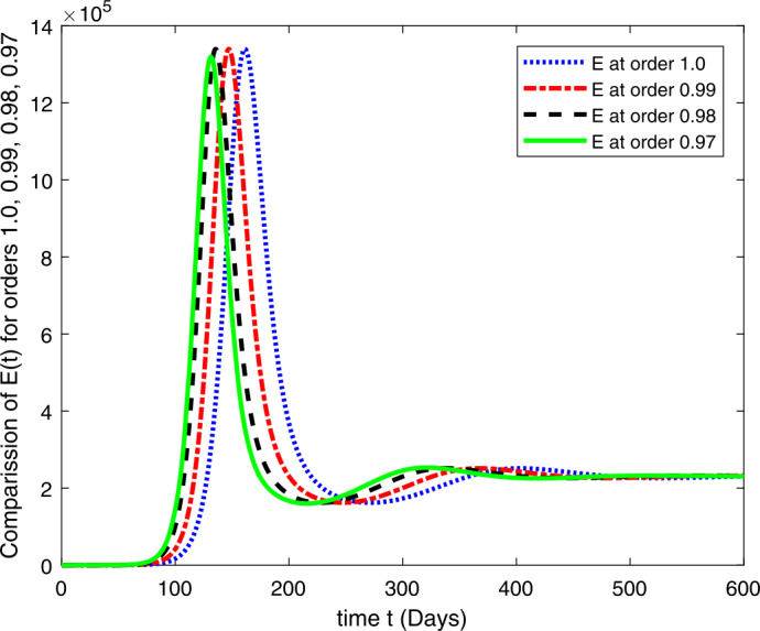
The computational results are given via ten graphs. In the Fig. 1, we have given the numerical solution of the suggested model for order 1 which is compared with the numerical solution of the model for orders 0.99, 0.98, 0.97 in Figs. 2, 3 and 4, respectively. Figure 5 is for the comparative study of $S(t)$ for the different orders. Similarly, $E(t)$, $I_s(t)$, $I_h(t)$, $A(t)$ and $R(t)$ are analysed for different fractional orders in the Figs. 6, 7, 8, 9, and 10 respectively.

Figure 1.

Joint solution of COVID 19 model (1) for the order 1.0

Figure 2.

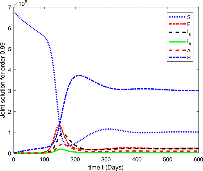
Joint solution of COVID 19 model (1) for the order 0.99

Figure 3.

Joint solution of COVID 19 model (1) for the order 0.98

Figure 4.

Joint solution of COVID 19 model (1) for the order 0.97

Figure 5.

Computational results for $S(t)$ while the fractional orders are 1.0, 0.99, 0.98, 0.97

Figure 6.

A comparative analysis of $E(t)$ for the fractional orders 1.0, 0.99, 0.98, 0.97

Figure 7.

Computational results for $I_s(t)$ for the fractional orders 1.0, 0.99, 0.98, 0.97

Figure 8.

A comparative analysis of $I_h(t)$ for the fractional orders 1.0, 0.99, 0.98, 0.97

Figure 9.

A comparative analysis of $A(t)$ for the fractional orders 1.0, 0.99, 0.98, 0.97

Figure 10.

A comparative analysis of $R(t)$ for the fractional orders 1.0, 0.99, 0.98, 0.97

Conclusion

In current manuscript, we have established a detailed analysis related to the results about existence and uniqueness results with Ulam stability. The subjective problem is nonlocal multipoint BVPs involving delay term of FDEs. The respective analysis has been established via using classical fixed point theory and some results of nonlinear functional analysis. The whole analysis has been demonstrated via computational results based on the literature. The initial values for the population are: $S(0)=6,778,382$, $E(0)=1$, $I_s(0)=0$, $I_h(0)=0$, $A(0)=0$, $R(0)=0$, and the parametric values are: $b_1=57,554$, $b_2=1/85$, $N=6,778,383$, $\beta =1/N$, ${\beta }_{a}r=1$, ${\beta }_{h}r=1/80$, $\gamma =1/5.5$, $\eta =0$, $\alpha =0.12$, ${\tau }_0=1/10$, $p_s=0.55$, $p_h=0.20$, $k_v=0.001$, $k_T=0.004$ [37]. The results are more realistic and of the same behavior as the classical ones. Our results are getting more similar to the integer order ones for the orders closer to 1.0.

Authors’ contributions

All authors have equal contribution in this paper. All authors read and approved the final manuscript.

Funding

Not applicable.

Availability of data and materials

No data were used to support this study.

Competing interests

The authors declare that they have no competing interests.

References

- 1.Lu H., Stratton C.W., Tang Y.W. Outbreak of pneumonia of unknown etiology in Wuhan China: the mystery and the miracle. J. Med. Virol. 2020;92(04):401–402. doi: 10.1002/jmv.25678. [DOI] [PMC free article] [PubMed] [Google Scholar]
- 2. Zimmer, C., Corum, J., Wee, S.-L.: Coronavirus Vaccine Tracker (2020) https://www.nytimes.com/interactive/2020/science/coronavirus-vaccine-tracker.html
- 3. CDC December: (2020) https://www.cdc.gov/coronavirus/2019-ncov/vaccines/different-vaccines.html
- 4.Goyal M., Baskonus H.M., Prakash A. An efficient technique for a time fractional model of Lassa hemorrhagic fever spreading in pregnant women. Eur. Phys. J. Plus. 2019;134(481):1–10. [Google Scholar]
- 5.Gao W., Veeresha P., Prakasha D.G., Baskonus H.M., Yel G. New approach for the model describing the deathly disease in pregnant women using Mittag-Leffler function. Chaos Solitons Fractals. 2020;134:109696. doi: 10.1016/j.chaos.2020.109696. [DOI] [Google Scholar]
- 6.Kumar D., Singh J., Al-Qurashi M., Baleanu D. A new fractional SIRS-SI malaria disease model with application of vaccines, anti-malarial drugs, and spraying. Adv. Differ. Equ. 2019;278:1–10. [Google Scholar]
- 7.Shah K., Alqudah M.A., Jarad F., Abdeljawad T. Semi-analytical study of Pine Wilt disease model with convex rate under Caputo-Fabrizio fractional order derivative. Chaos Solitons Fractals. 2020;135:109754. doi: 10.1016/j.chaos.2020.109754. [DOI] [Google Scholar]
- 8.Pang J., Cui J.A., Zhou X. Dynamical behavior of a Hepatitis B virus transmission model with vaccination. J. Theor. Biol. 2010;265(4):572–578. doi: 10.1016/j.jtbi.2010.05.038. [DOI] [PubMed] [Google Scholar]
- 9.Zou L., Zhang W., Ruan S. Modeling the transmission dynamics and control of Hepatitis B virus in China. J. Theor. Biol. 2010;262(2):330–338. doi: 10.1016/j.jtbi.2009.09.035. [DOI] [PubMed] [Google Scholar]
- 10.Chen T.-M., Rui J., Wang Q.-P., Zhao Z.-Y., Cui J.-A., Yin L. A mathematical model for simulating the phase-based transmissibility of a novel coronavirus. Infect. Dis. Poverty. 2020;9:24. doi: 10.1186/s40249-020-00640-3. [DOI] [PMC free article] [PubMed] [Google Scholar]
- 11.Zhou P., Yang X., Wang X., et al. A pneumonia outbreak associated with a new coronavirus of probable bat origin. Nature. 2020;579:270273. doi: 10.1038/s41586-020-2012-7. [DOI] [PMC free article] [PubMed] [Google Scholar]
- 12.Li Q., Guan X., Wu P., et al. Early transmission dynamics in Wuhan, China, of novel coronavirus 221 infected pneumonia. N. Engl. J. Med. 2020;382:1199–1207. doi: 10.1056/NEJMoa2001316. [DOI] [PMC free article] [PubMed] [Google Scholar]
- 13.Huang C., Wang Y., et al. Clinical features of patients infected with 2019 novel coronavirus in Wuhan China. Lancet. 2020;395:497–506. doi: 10.1016/S0140-6736(20)30183-5. [DOI] [PMC free article] [PubMed] [Google Scholar]
- 14.Podlubny I. Fractional Differential Equations, Mathematics in Science and Engineering. New York: Academic Press; 1999. [Google Scholar]
- 15.Lakshmikantham V., Leela S., Vasundhara J. Theory of Fractional Dynamic Systems. Cambridge: Cambridge Academic Pub.; 2009. [Google Scholar]
- 16.Rossikhin Y.A., Shitikova M.V. Applications of fractional calculus to dynamic problems of linear and nonlinear hereditary mechanics of solids. Appl. Mech. Rev. 1997;50:15–67. doi: 10.1115/1.3101682. [DOI] [Google Scholar]
- 17.Machado J., Kiryakova V., Mainardi V. Recent history of fractional calculus. Commun. Nonlinear Sci. Numer. Simul. 2011;16(3):4756–4767. doi: 10.1016/j.cnsns.2010.05.027. [DOI] [Google Scholar]
- 18.Baleanu D., Diethelm K., Scalas E., Trujillo J. Fractional Calculus Models and Numerical Methods. Singapore: World Scientific; 2012. [Google Scholar]
- 19.Heymans N., Bauwens J. Fractal rheological models and fractional differential equations for viscoelastic behaviour. Rheol. Acta. 1994;33:210–219. doi: 10.1007/BF00437306. [DOI] [Google Scholar]
- 20.Mainardi F. Fractional Calculus and Waves in Linear Viscoelasticity. London: Imperial College Press; 2010. [Google Scholar]
- 21.Machado J.T., Kiryakova V., Mainardi F. Recent history of fractional calculus. Commun. Nonlinear Sci. Numer. Simul. 2011;16(3):1140–1153. doi: 10.1016/j.cnsns.2010.05.027. [DOI] [Google Scholar]
- 22. Loverro, A.: Fractional calculus: history, definitions and applications for the engineer. Rapport Technique, Univeristy of Notre Dame: Department of Aerospace and Mechanical Engineering, Dame (2004)
- 23.Osler T.J. Fractional derivatives and Leibniz rule. Am. Math. Mon. 1971;78(6):645–649. doi: 10.1080/00029890.1971.11992819. [DOI] [Google Scholar]
- 24.Malinowska A.B., Odzijewicz T., Torres D.F. Advanced Methods in the Fractional Calculus of Variations. Cham: Springer; 2015. [Google Scholar]
- 25.Kilbas A.A., Srivastava H.M., Trujillo J.J. Factorization, Singular Operators and Related Problems. Dordrecht: Springer; 2003. Fractional differential equations: a emergent field in applied and mathematical sciences; pp. 151–173. [Google Scholar]
- 26.Jumarie G. Modified Riemann Liouville derivative and fractional Taylor series of nondifferentiable functions further results. Comput. Math. Appl. 2006;51(9–10):1367–1376. doi: 10.1016/j.camwa.2006.02.001. [DOI] [Google Scholar]
- 27.Algahtani O.J. Comparing the Atangana Baleanu and Caputo Fabrizio derivative with fractional order: Allen Cahn model. Chaos Solitons Fractals. 2016;1(89):552–559. doi: 10.1016/j.chaos.2016.03.026. [DOI] [Google Scholar]
- 28.Kao Y., Gao C., Wang D. Global exponential stability of reaction-diffusion Hopfield neural networks with continuously distributed delays. J. Math. Anal. Appl. 2008;21(3):457–462. [Google Scholar]
- 29.Luo J. Fixed points and exponential stability of mild solutions of stochastic partial differential equations with delays. J. Math. Anal. Appl. 2008;342(2):753–760. doi: 10.1016/j.jmaa.2007.11.019. [DOI] [Google Scholar]
- 30.Wang L. Global well-posedness and stability of the mild solutions for a class of stochastic partial functional differential equations. Sci. China Math. 2017;47(3):371–382. [Google Scholar]
- 31.Wang L., Gao Y. Global exponential robust stability of reaction diffusion interval neural networks with time-varying delays. Phys. Lett. A. 2006;350(56):342–348. doi: 10.1016/j.physleta.2005.10.031. [DOI] [Google Scholar]
- 32.Wang L., Zhang R., Wang Y. Global exponential stability of reaction-diffusion cellular neural networks with S-type distributed time delays. Nonlinear Anal., Real World Appl. 2009;10(2):1101–1113. doi: 10.1016/j.nonrwa.2007.12.002. [DOI] [Google Scholar]
- 33.Lu J.G. Global exponential stability and periodicity of reaction diffusion delayed recurrent neural networks with Dirichlet boundary conditions. Chaos Solitons Fractals. 2008;35(1):116–125. doi: 10.1016/j.chaos.2007.05.002. [DOI] [Google Scholar]
- 34.Atangana A., Akgul A., Owolabi K.M. Analysis of fractal fractional differential equations. Alex. Eng. J. 2020;59(3):1117–1134. doi: 10.1016/j.aej.2020.01.005. [DOI] [Google Scholar]
- 35.Chen W. A speculative study of 2/3-order fractional Laplacian modeling of turbulence: some thoughts and conjectures. Chaos. 2006;16:023126. doi: 10.1063/1.2208452. [DOI] [PubMed] [Google Scholar]
- 36.Meerschaert M.M., Tadjeran C. Finite difference approximations for fractional advection dispersion flow equations. J. Comput. Appl. Math. 2004;172:65–77. doi: 10.1016/j.cam.2004.01.033. [DOI] [Google Scholar]
- 37.Djomegni P.M., Haggar M.D., Adigo W.T. Mathematical model for Covid-19 with “protected susceptible” in the post-lockdown era. Alex. Eng. J. 2021;60(1):527–535. doi: 10.1016/j.aej.2020.09.028. [DOI] [Google Scholar]
- 38.Alqahtani B., Aydi H., Karapinar E., Rakocevic V. A solution for Volterra fractional integral equations by hybrid contractions. Mathematics. 2019;7(8):694. doi: 10.3390/math7080694. [DOI] [Google Scholar]
- 39.Karapinar E., Fulga A., Rashid M., Shahid L., Aydi H. Large contractions on quasi-metric spaces with an application to nonlinear fractional differential equations. Mathematics. 2019;7(5):444. doi: 10.3390/math7050444. [DOI] [Google Scholar]
- 40.Baleanu D., Jajarmi A., Mohammadi H., Rezapour S. A new study on the mathematical modelling of human liver with Caputo–Fabrizio fractional derivative. Chaos Solitons Fractals. 2020;134:109705. doi: 10.1016/j.chaos.2020.109705. [DOI] [Google Scholar]
- 41.Tuan N.H., Mohammadi H., Rezapour S. A mathematical model for COVID-19 transmission by using the Caputo fractional derivative. Chaos Solitons Fractals. 2020;140:110107. doi: 10.1016/j.chaos.2020.110107. [DOI] [PMC free article] [PubMed] [Google Scholar]
- 42.Mohammadi H., Kumar S., Rezapour S., Etemad S. A theoretical study of the Caputo–Fabrizio fractional modeling for hearing loss due to Mumps virus with optimal control. Chaos Solitons Fractals. 2021;144:110668. doi: 10.1016/j.chaos.2021.110668. [DOI] [Google Scholar]
- 43. Mohammadi, H., Rezapour, S., Jajarmi, A.: On the fractional SIRD mathematical model and control for the transmission of COVID-19: the first and the second waves of the disease in Iran and Japan. ISA Trans. (2021) [DOI] [PMC free article] [PubMed]
- 44.Baleanu D., Etemad S., Rezapour S. A hybrid Caputo fractional modeling for thermostat with hybrid boundary value conditions. Bound. Value Probl. 2020;2020(1):1. doi: 10.1186/s13661-020-01361-0. [DOI] [Google Scholar]
- 45.Shaikh A.S., Shaikh I.N., Nisar K.S. A mathematical model of COVID-19 using fractional derivative: outbreak in India with dynamics of transmission and control. Adv. Differ. Equ. 2020;2020(1):1. doi: 10.1186/s13662-020-02834-3. [DOI] [PMC free article] [PubMed] [Google Scholar]
- 46.Singh H., Srivastava H.M., Hammouch Z., Nisar K.S. Numerical simulation and stability analysis for the fractional-order dynamics of COVID-19. Results Phys. 2021;20:103722. doi: 10.1016/j.rinp.2020.103722. [DOI] [PMC free article] [PubMed] [Google Scholar]
- 47.Baba I.A., Yusuf A., Nisar K.S., Abdel-Aty A.H., Nofal T.A. Mathematical model to assess the imposition of lockdown during COVID-19 pandemic. Results Phys. 2021;20:103716. doi: 10.1016/j.rinp.2020.103716. [DOI] [PMC free article] [PubMed] [Google Scholar]
- 48.Aghdaoui H., Alaoui A.L., Nisar K.S., Tilioua M. On analysis and optimal control of a SEIRI epidemic model with general incidence rate. Results Phys. 2021;20:103681. doi: 10.1016/j.rinp.2020.103681. [DOI] [Google Scholar]
- 49.Panda S.K., Ravichandran C., Hazarika B. Results on system of Atangana-Baleanu fractional order Willis aneurysm and nonlinear singularly perturbed boundary value problems. Chaos Solitons Fractals. 2021;142:110390. doi: 10.1016/j.chaos.2020.110390. [DOI] [Google Scholar]
- 50. Logeswari, K., Ravichandran, C., Nisar, K.S.: Mathematical model for spreading of COVID-19 virus with the Mittag-Leffler kernel. Numer. Methods Partial Differ. Equ. (2020) [DOI] [PMC free article] [PubMed]
- 51.Valliammal N., Ravichandran C., Nisar K.S. Solutions to fractional neutral delay differential nonlocal systems. Chaos Solitons Fractals. 2020;138:109912. doi: 10.1016/j.chaos.2020.109912. [DOI] [Google Scholar]
Associated Data
This section collects any data citations, data availability statements, or supplementary materials included in this article.
Data Availability Statement