Performance Comparison of Compressed Sensing Algorithms for Accelerating T_1ρ Mapping of Human Brain

Abstract

Background:

3D-T_1ρ mapping is useful to quantify various neurologic disorders, but data are currently time-consuming to acquire.

Purpose:

To compare the performance of five compressed sensing (CS) algorithms—spatiotemporal finite differences (STFD), exponential dictionary (EXP), 3D-wavelet transform (WAV), low-rank (LOW) and low-rank plus sparse model with spatial finite differences (L + S SFD)—for 3D-T_1ρ mapping of the human brain with acceleration factors (AFs) of 2, 5, and 10.

Study Type:

Retrospective.

Subjects:

Eight healthy volunteers underwent T_1ρ imaging of the whole brain.

Field Strength/Sequence:

The sequence was fully sampled 3D Cartesian ultrafast gradient echo sequence with a customized T_1ρ preparation module on a clinical 3T scanner.

Assessment:

The fully sampled data was undersampled by factors of 2, 5, and 10 and reconstructed with the five CS algorithms. Image reconstruction quality was evaluated and compared to the SENSE reconstruction of the fully sampled data (reference) and T_1ρ estimation errors were assessed as a function of AF.

Statistical Tests:

Normalized root mean squared errors (nRMSE) and median normalized absolute deviation (MNAD) errors were calculated to compare image reconstruction errors and T_1ρ estimation errors, respectively. Linear regression plots, Bland–Altman plots, and Pearson correlation coefficients (CC) are shown.

Results:

For image reconstruction quality, at AF = 2, EXP transforms had the lowest mRMSE (1.56%). At higher AF values, STFD performed better, with the smallest errors (3.16% at AF = 5, 4.32% at AF = 10). For whole-brain quantitative T_1ρ mapping, at AF = 2, EXP performed best (MNAD error = 1.62%). At higher AF values (AF = 5, 10), the STFD technique had the least errors (2.96% at AF = 5, 4.24% at AF = 10) and the smallest variance from the reference T_1ρ estimates.

Data Conclusion:

This study demonstrates the use of different CS algorithms that may be useful in reducing the scan time required to perform volumetric T_1ρ mapping of the brain.

Quantitative Mapping using T_1ρ contrast, the spin lattice relaxation time in the rotating reference frame, offers the ability to characterize tissue in unique ways and offer new insights to health and pathology. While routinely used in musculoskeletal applications,^1,2 T_1ρ contrast has also been applied to various brain imaging applications, including cerebral ischemia,³ Alzheimer’s disease,⁴ epilepsy,⁵ and multiple sclerosis.⁶ Additionally, the sensitivity of T_1ρ contrast to chemical exchange can potentially allow the characterization of myelin and multicomponent relaxation studies.⁷ A major challenge for quantitative T_1ρ mapping is the long scan times required to acquire multiple spin lock durations.² Additionally, applications that have explored biexponential and multicompartment modeling require additional spin-lock time (TSL) acquisitions that prolong the T_1ρ imaging time even further.^7,8 These long scan times result in an increased likelihood of motion-induced artifacts that corrupt data. Reducing the overall scan time for quantitative T_1ρ imaging, without sacrificing the TSL requirement, would enable its use for broad neuro applications.

The advent of compressed sensing (CS) has enabled magnetic resonance imaging (MRI) to cross the Nyquist barrier and to allow undersampling the data in order to reduce scan time.⁹ By a combination of image sparsity, incoherent sampling, and nonlinear reconstruction, CS techniques have been very useful in multiple imaging applications, including dynamic imaging^10,11 and multiparameter mapping.^12–14 Moreover, parallel imaging with multiple coils enhances the performance of CS techniques.¹⁵ A number of advances in T_1ρ mapping using CS have been developed.^16,17

Current approaches to reducing the time required for volumetric T_1ρ mapping can be broadly classified into two types. The first type employs a two-step approach to reconstruct images and then use conventional fitting methods for mapping of the desired parameters. A number of implementations use CS¹⁴ and low-rank methods,^18,19 or a combination of low-rank and sparsity to improve reconstruction.²⁰ The second type is called model-based reconstruction techniques and combines the relaxometry model into the image reconstruction.^21,22

There have been a number of studies investigating the utility of T_1ρ mapping in cartilage,^17,23 and the heart,²⁴ but only a few have explored the utility of CS for the application of T_1ρ mapping of the brain.^16,25 A study that compares the performance of multiple CS algorithms for T_1ρ mapping of the brain would be beneficial. The purpose of this study, therefore, was to evaluate the performance of different CS techniques at different acceleration factors (AFs) with respect to image quality errors and T_1ρ mapping errors to facilitate an informed choice of reconstruction algorithm for 3D T_1ρ mapping of the brain.

Materials and Methods

Subjects and Imaging Protocol

This prospective study was approved by the Institutional Review Board (IRB) and was Health Insurance Portability and Accountability Act (HIPAA)-compliant. The exclusion criteria consisted of no past history of major illnesses or surgery, and inclusion criteria required that the volunteers were over the age of 18 years. Eight healthy volunteers (four males, four females, age = 31.2 ± 5.9 years) were recruited following written informed consent. The MRI protocol consisted of whole-brain T_1ρ imaging using a fully sampled 3D-Cartesian turbo-FLASH sequence with a customized T_1ρ preparation pulse.^7,8 All scans were performed with a 3T clinical MRI scanner (Prisma, Siemens Healthineers, Erlangen, Germany) with a vendor-supplied 20-channel receive-only head-coil. The acquisition parameters were: repetition time (TR) = 5 msec, echo time (TE) = 2.9 msec, T₁ delay = 1 sec, field of view = 240 × 240 mm², matrix size = 256 × 128 × 64, in-plane spatial resolution = 0.94 × 0.94, axial orientation, flip angle = 8°, slice thickness = 2 mm, receiver bandwidth = 515 Hz/pixel, spin-lock frequency = 500 Hz, 10 TSLs = 2, 4, 6, 8, 10, 15, 25, 35, 45, 55 msec, total acquisition time = 32 minutes.

Reference Reconstruction With Fully Sampled Data

The fully sampled reconstruction images served as the reference, and the T_1ρ maps calculated from them served as the reference T_1ρ maps. One-dimensional Fourier transform was applied in the through-plane direction to simplify and improve efficiency and perform separate reconstructions for each slice. The reference images were reconstructed with the sensitivity encoding method (SENSE),²⁶ with coil sensitivity maps estimated using the ESPIRiT²⁷ algorithm, that used a fully sampled central k-space area.

Retrospective Undersampling

To test the performance of different CS algorithms, the fully sampled dataset was retrospectively undersampled to create versions that simulate AF of 2, 5, and 10, where AF is defined as the ratio of total samples in the fully sampled case to the samples used in the undersampled case. A 2D Poisson-disc with random sampling was used in the in-plane direction.⁹ A central fully sampled core consisting of size = 31 × 15 (AF = 2) or 21 × 9 (AF ≥5) was used for coil sensitivity estimation. The 2D sampling pattern was repeated for all slices in the through-plane direction.

Models and Fitting Algorithms

Figure 1 shows a schematic of the models used for reconstruction with their required inputs and outputs. For reconstruction of undersampled data, five CS reconstruction models were tested with differing regularization functions: spatial and temporal finite differences (STFD),²⁸ exponential dictionary (EXP),²⁹ 3D wavelet transform (WAV),³⁰ low-rank (LOW),³¹ and low-rank plus sparse model with spatial finite differences (LPS-SFD).²⁰

FIGURE 1:

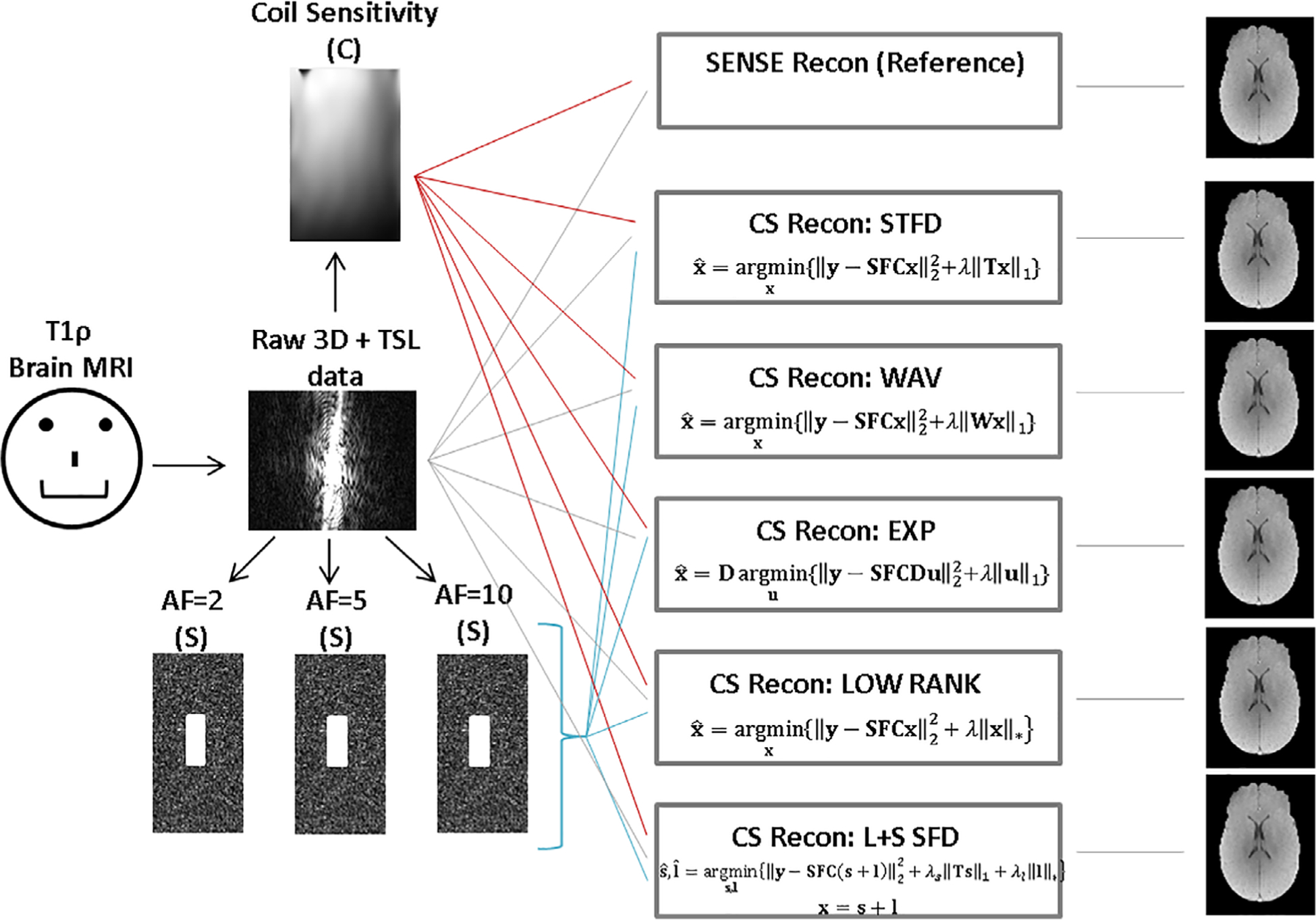
MRI reconstruction models. Raw data from fully sampled brain MRI data, coil sensitivity maps (C), and Fourier transform (F) were used as input to reconstruct the reference images using SENSE. A sampling matrix (S) which uses a 2D Poisson random undersampling is used to generate undersampled data with multiple acceleration factors (AFs). These are input to the reconstruction algorithms to generate respective output MR images.

The general form of all CS reconstructions was:

$$\widehat{\mathbf{x}}=\underset{\mathbf{x}}{\text{argmin}}\left\{\parallel \mathbf{y}-\mathbf{\text{SFCx}}{\parallel }_2^2+\lambda R(\mathbf{x})\right\}$$ (1)

where the first part is the data consistency term, where y is the acquired data, S is the sampling matrix, F is the Fourier transform, C represents the coil sensitivities, and x is the reconstructed object. The second part of the equation represents the regularization penalty where R(x) = Tx₁ is a sparsifying penalty where T represents the transform used. The STFD model uses spatial and temporal finite difference transforms with a temporal order of 1 and spatial order of 2. The STFD model imposes the spatial and temporal models together with the l₁-norm (Eq. 1). The 3D WAV model uses a 3D wavelet transform with an l₁-norm penalty for regularization. The EXP model (Eq. 2) uses an additional dictionary term D as part of the data consistency term, u is the reconstructed object in Eq. 2, where x = Du and the regularization term as the l₁-norm of the dictionary of exponentials:

$$\widehat{\mathbf{x}}=\underset{\mathbf{u}}{\mathbf{D}\text{argmin}}\left\{\parallel \mathbf{y}-\mathbf{\text{SFCDu}}{\parallel }_2^2+\lambda \parallel \mathbf{u}{\parallel }_1\right\}$$ (2)

For the LOW model, the data consistency term is as shown in Eq. 3, where the regularization penalty term utilizes a nuclear norm,³¹ the Casorati matrix of the reconstructed object:

$$\widehat{\mathbf{x}}=\underset{\mathbf{x}}{\text{argmin}}\left\{\parallel \mathbf{y}-\mathbf{\text{SFCx}}{\parallel }_2^2+\lambda \parallel \mathbf{x}{\parallel }_{*}\right\}$$ (3)

Finally, the LPS-SFD method (Eq. 4) consists of sparsity and low-rank terms, x=s + l, and the regularization penalty λR(x) from Eq. 1 is replaced by λR(s, l) = λ_s‖Ts‖₁ + λ_l‖l‖_* where the low-rank term, l, uses a nuclear norm, and the sparsity term, s uses an l₁-norm regularization penalty:

$$\widehat{\mathbf{s}},\widehat{\mathbf{l}}=\underset{\mathbf{s},\mathbf{\text{l}}}{\text{argmin}}\left\{\parallel \mathbf{y}-\mathbf{S}FC(\mathbf{s}+\mathbf{l}){\parallel }_2^2+{\lambda }_s\parallel \mathbf{T}s{\parallel }_1+{\lambda }_l\parallel \mathbf{\text{l}}{\parallel }_{*}\right\}$$ (4)

The regularization parameter λ was manually optimized for each technique. A test reconstruction was performed that used a log range of λ values and the optimized value of λ was determined. Since λ does not vary significantly within a particular technique, the same value was used for all subjects for each CS technique implemented. The regularization process aimed to minimize the l₂-norm of the difference between the particular CS technique and the reference technique. The cost-function minimization used the fast iterative shrinkage-thresholding algorithm (FISTA)³² with the fast gradient projection (FGP) algorithm.³³

FMRIB software library (FSL)³⁴ was used to strip the skull and generate whole-brain ROIs, which were used for T_1ρ mapping. Monoexponential T_1ρ mapping for each pixel was done after CS reconstruction using the nonlinear least squares fitting model, shown as:

$$S(\mathbf{r},TSL)=A(\mathbf{r})\cdot e^{\raisebox{1ex}{$-TSL$}\!\left/ \!\raisebox{-1ex}{$T_{1\rho }(\mathbf{r})$}\right.}+A_0,$$ (5)

where r is location of the voxel, A(r) is the amplitude, TSL are the spin lock durations used, T_1ρ(r) is rotating frame relaxation time, and A₀ is the calculated noise. A 3 × 3 denoising spatial prefilter³⁵ was used in each image uniformly prior to T_1ρ estimation process. Voxelwise quantitative T_1ρ maps were generated using the reference technique and each of the CS techniques used.

Subjective Evaluation of Accelerated Images Reconstructed from CS

To further evaluate the performance of the CS algorithms, three experienced observers R.J. (>15 years of experience) Y.G. (>15 years of experience), and R.G.M. (10 years of experience) independently (blinded to AFs and type of CS algorithm) scored the accelerated images reconstructed from CS algorithms against the fully sampled data as standard of reference along aspects of contrast, artifacts, and sharpness on a 3-point scale (1, least favorable, 2, adequate, and 3, most favorable). Similarly, the diagnostic quality of the accelerated images was scored against the reference on a 4-point scale (0, non-diagnostic, 1, poor, 2, adequate, and 3, good).

Data Analysis and Statistics

To compare the quality of the images from the CS reconstructions to reference images from the SENSE reconstruction, normalized root mean square error (nRMSE) was used, defined as follows:

$$\mathit{\text{nRMSE}}\left(\widehat{\mathit{x}},{\mathit{x}}_{Ref}\right)={‖\widehat{\mathit{x}}-{\mathit{x}}_{Ref}‖}_2/{‖{\mathit{x}}_{Ref}‖}_2$$ (6)

To compare the T_1ρ quantification results with the estimates from the fully sampled reference, voxelwise normalized absolute deviation (NAD) was calculated as:

$$NAD(\mathit{r})=\frac{\left|\widehat{p}(\mathit{r})-p_{Ref}(\mathit{r})\right|}{\left(\widehat{p}(\mathit{r})+p_{Ref}(\mathit{r})\right)/2}$$ (7)

where $\widehat{p}$ is the T_1ρ estimate, and p_Ref is the T_1ρ values calculated from the reference technique. The median of the NAD (MNAD)¹⁷ in the whole-brain ROIs was calculated as:

$$\mathit{\text{MNAD}}(ROI)=\underset{\mathit{r}\in ROI}{\mathit{\text{median}}}NAD(\mathit{r}).$$ (8)

Linear regression of mean values between reference and different CS methods for whole-brain ROIs were plotted. Bland–Altman plots comparing the agreement of the reference technique and the different CS methods were evaluated. In addition, the Pearson correlation coefficient between the reference values and the CS methods tested were calculated. Two-tailed t-tests were used to compare the significance of each correlation, with a significance threshold of 0.05.

Results

Reconstructed MR images from a representative slice for each of the CS algorithms tested, and for the AFs used in the study at TSL = 2 msec, are shown in Fig. 2. At higher AF, particularly at AF = 10, a loss of subtle image features is noted in all the CS reconstruction techniques. Figure 3 shows a comparison of reconstructed images for a representative slice for four of the 10 TSL values obtained, including the shortest spin lock duration (TSL = 2 msec), and the longest spin lock duration (TSL = 55 msec). Table 1 summarizes the CS algorithm image reconstruction performance compared to the SENSE technique as reference. The best-performing algorithm at each AF is highlighted in bold. Also shown in the table are average iterations taken for the minimization, and the average time taken for each algorithm.

FIGURE 2:

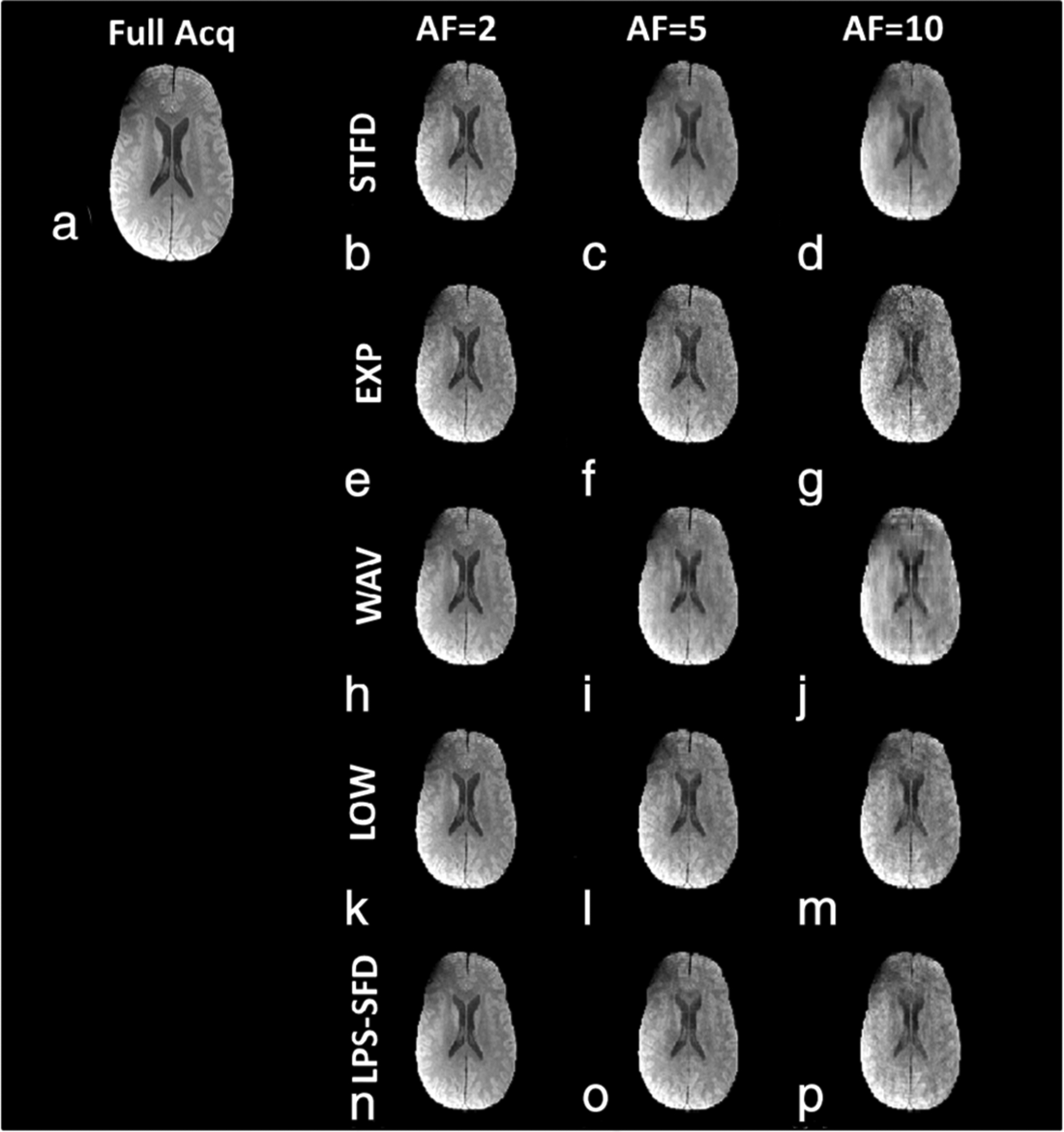
Retrospective reconstruction at different AFs. (a) The reference from SENSE reconstruction obtained from a fully sampled acquisition. (b–p) CS reconstructed images. Each row shows the reconstruction from a different CS reconstruction model, and columns 2–4 show different AF. All the images shown here are at TSL = 2 msec, the shortest spin lock time acquired.

FIGURE 3:

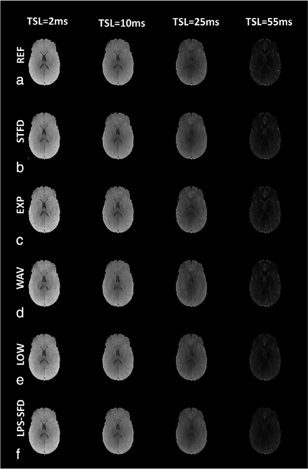
Retrospective reconstruction at multiple TSLs. Row of images in (a) show the reconstructed reference images at representative TSL values using SENSE reconstruction. Rows (b–f) show results at multiple TSL values using each of CS reconstruction algorithms used at AF = 2.

TABLE 1.

CS Algorithm Image Reconstruction Performance

	nRMSE (Images) (N = 8)
	AF=2	AF=5	AF=10	Average iterations	Average time (s)
STFD	0.0184	0.0329	0.0437	181	206 s
EXP	0.0158	0.0373	0.0595	400	153 s
WAV	0.0168	0.0323	0.0471	161	119 s
LOW	0.0174	0.0338	0.0479	200	75 s
LPS-SFD	0.0224	0.0363	0.0604	160	155 s

The table summarizes the nRMSE for the algorithms used at the AFs tested. The computational cost in the number of iterations used and the average time for those iterations are shown. The lowest errors for each AF are marked in bold.

The image quality comparison for the CS algorithms tested at different AF values are shown in Fig. 4. Figure 4a shows the SENSE reconstruction from a representative slice used as the reference. Images in Fig. 4b show the corresponding CS reconstruction at AF = 2; Fig. 4c shows the nRMSE for each technique at AF = 2. Figure 4d shows the CS reconstruction for each algorithm at AF = 10, and Fig. 4e shows the corresponding nRMSE at AF = 10. All the CS reconstruction algorithms showed a gradual increase in the nRMSE from AF = 2 to AF = 10, increasing from 0.015 to 0.06. Figure 4f shows the plot of nRMSE with AF for each CS algorithm. At AF = 2, the nRMSE in the EXP technique was the least at 0.0158. At AF ≥5, the least error was seen in the STFD technique, outperforming the other techniques at higher AF (nRMSE = 4.37% at AF = 10).

FIGURE 4:

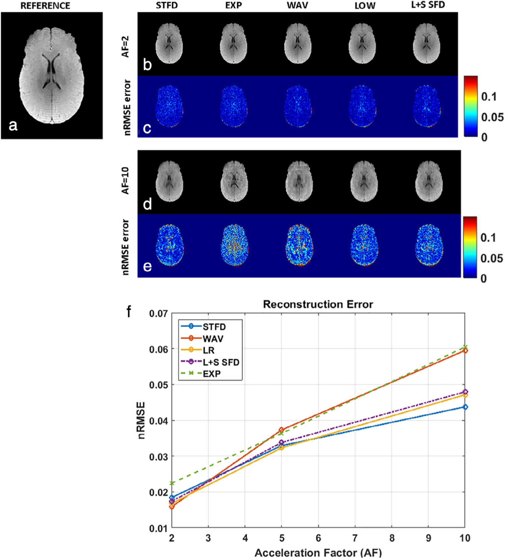
Image quality comparison at different AFs. (a) A representative reference image from SENSE reconstruction. (b) The corresponding CS reconstruction at AF = 2. (c) The nRMSE for each technique at AF = 2. (d) The CS reconstruction for each algorithm at AF = 10. (e) The corresponding nRMSE at AF = 10. The relative increases in nRMSE from AF = 2 to AF = 10 among the different algorithms can be seen. (f) The plot of nRMSE with AF for each CS algorithm. At higher AF, STFD has the least error.

Comparison of image reconstruction results in two representative subjects are shown in Fig. 5. Figure 5a shows a representative reference image from SENSE reconstruction for subject 1; Fig. 5b shows the corresponding CS reconstruction for each CS reconstruction using AF = 5, and Fig. 5c shows the nRMSE for the corresponding technique. Similarly, for subject 2, Fig. 5d is the reference image; Fig. 5e is CS reconstruction at AF = 5; and Fig. 5f shows the nRMSE for each technique at AF = 5. The results demonstrate similar algorithm performance between subjects.

FIGURE 5:

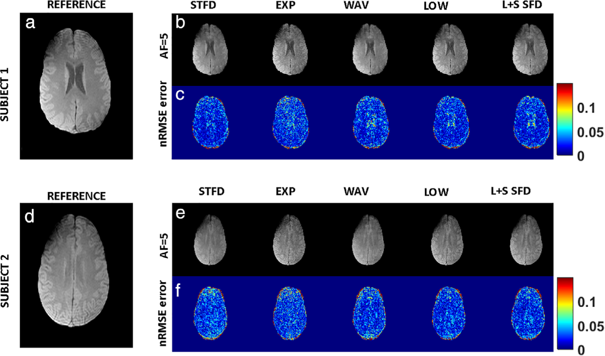
Intersubject comparison. For subject 1, (a) shows a representative reference image from SENSE reconstruction, (b) shows the corresponding CS reconstruction for each CS reconstruction using AF = 5, and (c) shows the nRMSE for the corresponding technique. Similarly, for subject 2, (d) is the reference image, (e) is CS reconstruction at AF = 5, and (f) shows the nRMSE for each technique at AF = 5.

Figure 6 shows a comparison of image reconstruction performance at different spin lock durations. At TSL = 2 msec, Fig. 6a shows a representative reference image; Fig. 6b shows CS reconstructed images with the algorithms tested at AF = 2; and Fig. 6c shows the corresponding nRMSE. Figure 6d–f shows the corresponding set of images for a mid-range spin lock duration (TSL = 25 msec), and Fig. 6g,h shows the reference image, CS image reconstruction, and the corresponding nRMSE at the longest spin lock duration (TSL = 55 msec). At the longest TSL of 55 msec, with increasing noise in both the SENSE reconstructed reference image and the corresponding CS reconstruction, there is considerable divergence in the performance among the different algorithms tested.

FIGURE 6:

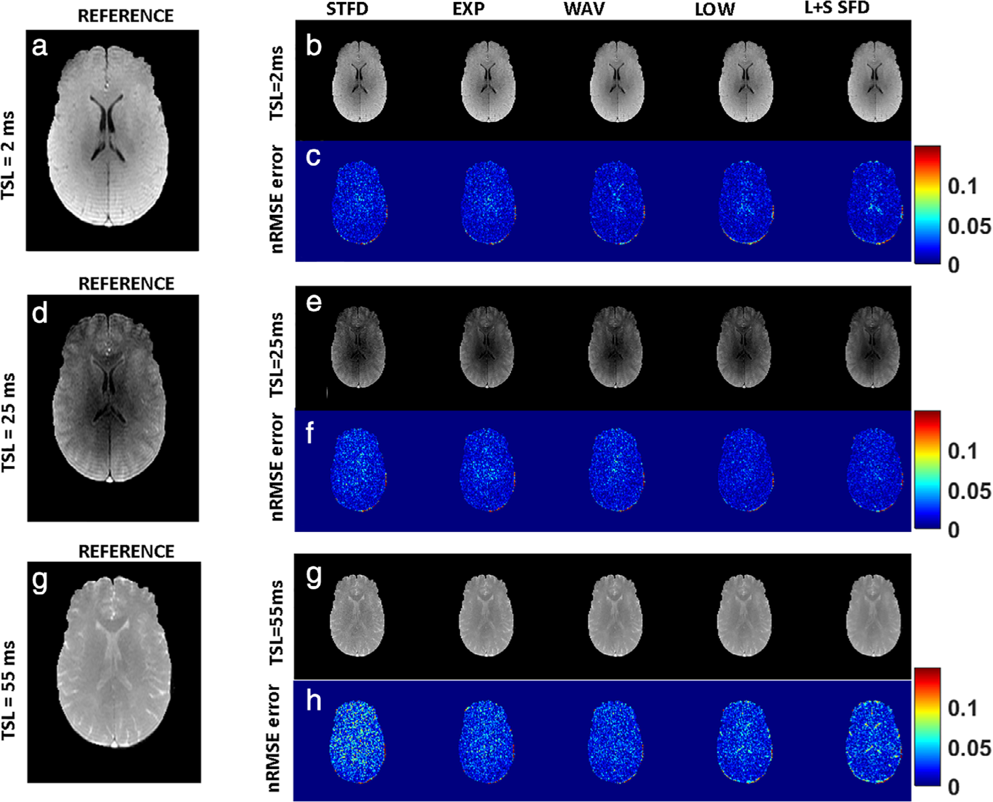
Performance comparison at different spin lock durations. At TSL = 2 msec, (a–c) show a representative reference image, CS reconstructed images with the algorithms tested at AF = 2, and the corresponding nRMSE, respectively. (d–f) The corresponding set of images at TSL = 25 msec, and (g,h) the corresponding set of images at TSL = 55 msec. At the longest TSL of 55 msec, with increasing noise in both the SENSE reconstructed reference image and the corresponding CS reconstruction, there is considerable divergence in the performance among the different algorithms tested.

Performance comparison of T_1ρ estimation with the reference technique are shown in Fig. 7. For subject 1, Fig. 7a shows a representative slice of the reference T_1ρ map; Fig. 7b shows estimated T_1ρ maps using the CS algorithms tested at AF = 5; and Fig. 7c shows the corresponding NAD error for each technique. Similarly, for subject 2, Fig. 7d–f shows the reference T_1ρ map, estimated T_1ρ maps at AF = 5 for each CS method, and the corresponding NAD errors for each technique, respectively.

FIGURE 7:

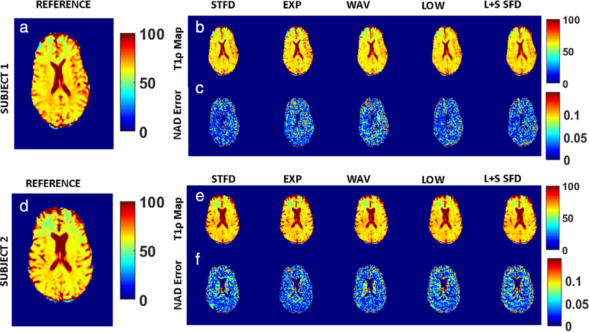
T_1ρ estimation performance comparison. For subject 1, (a) shows a representative slice of the estimated T_1ρ map that is used as reference, (b) shows estimated T_1ρ maps using the CS algorithms tested at AF = 5, and (c) shows the corresponding NAD error for each technique. Similarly, for subject 2, (d–f) show the reference T_1ρ map, estimated T_1ρ maps at AF = 5 for each CS method, and the corresponding NAD errors for each technique, respectively.

Results of the voxelwise comparison of T_1ρ maps from the fully sampled reference data compared to the CS reconstructed data are shown in Fig. 8. Subparts Fig. 8a–c shows the boxplots of the NAD error in T_1ρ estimation with AF values of 2, 5, and 10, respectively. While the median NAD error is similar across all the CS techniques, it is in the EXP technique (0.0146) at AF = 2, and least for the STFD technique at AF = 5 (0.0292) and 10 (0.0419). Additionally, the interquartile range, a measure of the variance of the estimates from the reference, was the least for the STFD technique at AF = 5 and 10. At AF = 10, LOW performed equally well (MNAD error = 4.19%). Figure 8d shows the MNAD error at different AFs using the reference T_1ρ estimates. Table 2 summarizes the performance of the CS methods with the T_1ρ estimation errors at different AFs.

FIGURE 8:

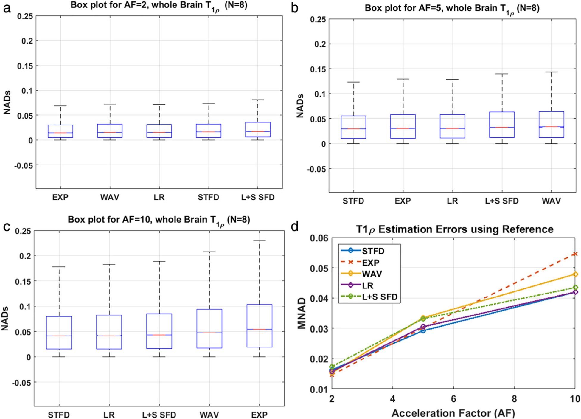
T_1ρ estimation errors. Boxplots of NAD error are shown for (a) AF = 2, (b) AF = 5, (c) AF = 10. (d) The T_1ρ estimation errors (MNAD) using the reference T_1ρ maps. Results for STFD perform the best for the highest AF.

Table 2.

T_1ρ Estimation Errors

	MNAD error (T1ρ) (N = 8)
	AF=2	AF=5	AF=10
STFD	0.0162	0.0292	0.0419
EXP	0.0146	0.0301	0.0546
WAV	0.0153	0.0334	0.0479
LOW	0.0157	0.0305	0.0419
L+S SFD	0.0173	0.0331	0.0434

The table summarizes the MNAD error for the algorithms used at the AFs tested. The lowest errors for each AF are marked in bold.

Figure S1 in the Supplemental Material shows the results of the independent reviewer scores. The scores predictably went lower for higher AFs across all CS algorithms. Similar to numerical analysis, images from the STFD and LOW technique scored the highest relative to other methods for contrast and artifacts. EXP performed better on sharpness. In terms of diagnostic quality across the all AFs, the STFD, EXP, and LOW algorithms performed equally well.

Figure S2 in the Supplemental Material shows the manual determination of the parameter λ. For each undersampled CS reconstruction and for each subject, a log range of λ was tested, and the error cost-function was determined. The optimized value of λ is then kept constant for all AFs tested. Linear regression plots between reference and the different CS methods used are shown for AF of 2, 5, and 10 (Fig. S3a–c in the Supplemental Material). Bland–Altman plots are shown in Fig. S3d–f in the Supplemental Material. All methods closely align with reference values, with a small non-significant drift seen at higher AF values. Table S1 in the Supplemental Material shows the Pearson correlation coefficient for each method compared with the reference with the corresponding P-values. The CC’s for each method are highly correlated with high significance (P < 0.05) for all methods tested.

Discussion

In this study we compared the performance of five CS algorithms for brain T_1ρ mapping and compared it with a reference SENSE reconstruction technique. To compare image reconstruction quality performance, we calculated the nRMSE between the different undersampled CS techniques and the fully sampled reference image. Similarly, to compare the T_1ρ error, the MNAD error between the different undersampled CS methods and the fully sampled reference map was calculated.

The image reconstruction performance at lower AF values (AF = 2) was best for the EXP technique. With the least nRMSE this would be the recommended technique for reconstructing brain images at AF = 2. Of note, however, two other techniques performed similarly but with slightly higher error, the low-rank technique and the WAV technique. At higher AFs (AF = 5 or 10) the STFD technique demonstrated the most robust performance compared to the reference. At AF = 5, all of the techniques tested showed similar performance, but at greater undersampling (AF = 10) the STFD performed clearly better than the other techniques when compared to the reference. The STFD technique incorporates spatial and temporal correlations in the T_1ρ data to achieve its performance, with temporal order set to 1 and spatial order set to 2.

The T_1ρ mapping performance at lower AF values (AF = 2) showed that the EXP technique worked best giving the lowest MNAD error. The MNAD error of the WAV technique at AF = 2 was very similar. At higher AF (≥5) the STFD performed the best, with the least MNAD error compared to reference. While the performance of the STFD was the best at AF = 5, all the other four techniques performed similarly. At higher AF (=10) the STFD and LOW technique were clearly better than the others compared to the reference, with lower MNAD error and lower variance compared to other CS techniques. Hence, the STFD or LOW technique should be the method of choice for higher AF values for T_1ρ brain mapping. Note that these results are specific to this imaging application, and may not extend to other applications. The L + S SFD method perform very close to the STFD technique at AF = 10, with slightly higher MNAD errors. One caveat to the recommendations here is the assumption that the reference technique is a good substitute for the ground truth. When the ground truth is not known, the fully sampled reference technique may be the only choice. Synthetic phantom experiments performed previously by Zibetti et al¹⁷ comparing the performance of T_1ρ estimates in noisy reference methods compared to ground truth showed that noisy data can contribute as much 4.2% MNAD error to the results. Another aspect that boosts the performance of the T_1ρ estimates across all CS techniques was the image denoising prefilter. In this study the image filter size was held constant at 3 × 3 voxels. It has been demonstrated previously that a 3 × 3 filter performs better than no filter and marginally better than a 5 × 5 voxel filter.¹⁷

Zhu et al³⁶ reported a principal component analysis (PCA)-based dictionary learning technique for brain T_1ρ mapping and reported T_1ρ errors up to 8.9% at AF = 4. Although we did not test the specific CS method used in that study, and we reported MNAD errors for T_1ρ mapping, the errors we report here are considerably lower at a comparable AF of 5. Bhave et al¹⁶ reported a blind compressed sensing (BCS) technique for brain T_1ρ mapping. Our study does not directly compare with the BCS techniques, but they reported a promising technique that was robust to motion, reporting T_1ρ estimation errors of 2.3% at AF = 8 without motion, and an error of 6.3% at AF = 8 with motion. In Zhu et al,²⁵ the authors used a variation of the L + S approach for brain T_1ρ mapping, testing with an AF up to 5, and reported nRMSE values around 0.01. The results from this study suggested that the STFD technique worked better than L + S for this application. In a more recent paper by Zhu et al,³⁷ a variable rate sampled L + S technique for biexponential brain T_1ρ mapping was used with a T_1ρ estimation error as low as 2.3% for AF = 6, which is slightly better than the error we report at a comparable AF of 5.

A number of studies have reported CS techniques applied to T_1ρ mapping of cartilage imaging applications. Pandit et al³⁸ reported knee cartilage errors less than 5% using a finite differences-based CS technique, with AF values up to 2.3. Zhou et al²³ used a CS technique that alternated iteratively between PCA and sensitivity estimation and were able to achieve significantly lower error rates (below 1%) in the T_1ρ mapping of knee cartilage. Zhang et al³⁹ implemented a modification of low-rank techniques for brain diffusion imaging, and reported errors ranging from 4.8–30.4% for AFs ranging from 2–8. Zibetti et al¹⁷ compared monoexponential knee cartilage using a similar comparison study and reported slightly higher error rates at AF of 10.

Limitations

CS works best if there is an objective ground truth to compare against. Because we used a reference technique that is noisy, the errors reported here may be subject to a correction factor that is not accounted for. This study compares the performance of a set of popular CS reconstruction algorithms reported in the literature, but it is not comprehensive. A number of additional regularization techniques exist that were not a part of this study, but an attempt was made to use the most promising ones for this application. Poisson sampling may not be the optimal choice of data acquisition for prospective acquisitions. This study was a relatively smaller study with eight young healthy volunteers. Greater numbers in the study population, with more diverse age range and pathologies, will provide greater insights. This study used full sampling with retrospective undersampling. Prospective undersampling will provide more insight into the experimental issues involved.

Conclusion

At AF = 2, the particular choice of CS algorithm may not make a big difference; at higher AF of greater than 5, the STFD technique outperforms the other techniques compared here. For STFD, the combination of first-order temporal and second-order spatial finite differences provides excellent performance, but the regularization parameters have to be manually optimized. The low rank and L + S SFD were a close second choice at higher AFs. The results of the study suggest that significant acceleration of brain T_1ρ mapping may be feasible with CS reconstruction with a proper choice of CS reconstruction.

References

- 1.Keenan KE, Besier TF, Pauly JM, et al. Prediction of glycosaminoglycan content in human cartilage by age, T1rho and T2 MRI. Osteoarthritis Cartilage 2011;19(2):171–179. [DOI] [PMC free article] [PubMed] [Google Scholar]
- 2.Wang L, Regatte RR. T(1)rho MRI of human musculoskeletal system. J Magn Reson Imaging 2015;41(3):586–600. [DOI] [PMC free article] [PubMed] [Google Scholar]
- 3.Jokivarsi KT, Hiltunen Y, Grohn H, Tuunanen P, Grohn OH, Kauppinen RA. Estimation of the onset time of cerebral ischemia using T1rho and T2 MRI in rats. Stroke 2010;41(10):2335–2340. [DOI] [PubMed] [Google Scholar]
- 4.Borthakur A, Sochor M, Davatzikos C, Trojanowski JQ, Clark CM. T1rho MRI of Alzheimer’s disease. Neuroimage 2008;41(4):1199–1205. [DOI] [PMC free article] [PubMed] [Google Scholar]
- 5.Deoni SC. Quantitative relaxometry of the brain. Top Magn Reson Imaging 2010;21(2):101–113. [DOI] [PMC free article] [PubMed] [Google Scholar]
- 6.Zipp F. A new window in multiple sclerosis pathology: Non-conventional quantitative magnetic resonance imaging outcomes. J Neurol Sci 2009;287(Suppl 1):S24–S29. [DOI] [PubMed] [Google Scholar]
- 7.Menon RG, Sharafi A, Windschuh J, Regatte RR. Bi-exponential 3D-T1rho mapping of whole brain at 3T. Sci Rep 2018;8(1):1176. [DOI] [PMC free article] [PubMed] [Google Scholar]
- 8.Sharafi A, Chang G, Regatte RR. Bi-component T1rho and T2 relaxation mapping of skeletal muscle in-vivo. Sci Rep 2017;7(1):14115. [DOI] [PMC free article] [PubMed] [Google Scholar]
- 9.Lustig M, Donoho D, Pauly JM. Sparse MRI: The application of compressed sensing for rapid MR imaging. Magn Reson Med 2007;58(6): 1182–1195. [DOI] [PubMed] [Google Scholar]
- 10.Feng L, Srichai MB, Lim RP, et al. Highly accelerated real-time cardiac cine MRI using k-t SPARSE-SENSE. Magn Reson Med 2013;70(1):64–74. [DOI] [PMC free article] [PubMed] [Google Scholar]
- 11.Feng L, Grimm R, Block KT, et al. Golden-angle radial sparse parallel MRI: Combination of compressed sensing, parallel imaging, and golden-angle radial sampling for fast and flexible dynamic volumetric MRI. Magn Reson Med 2014;72(3):707–717. [DOI] [PMC free article] [PubMed] [Google Scholar]
- 12.Doneva M, Bornert P, Eggers H, Stehning C, Senegas J, Mertins A. Compressed sensing reconstruction for magnetic resonance parameter mapping. Magn Reson Med 2010;64(4):1114–1120. [DOI] [PubMed] [Google Scholar]
- 13.Huang C, Graff CG, Clarkson EW, Bilgin A, Altbach MI. T2 mapping from highly undersampled data by reconstruction of principal component coefficient maps using compressed sensing. Magn Reson Med 2012;67(5):1355–1366. [DOI] [PMC free article] [PubMed] [Google Scholar]
- 14.Velikina JV, Alexander AL, Samsonov A. Accelerating MR parameter mapping using sparsity-promoting regularization in parametric dimension. Magn Reson Med 2013;70(5):1263–1273. [DOI] [PMC free article] [PubMed] [Google Scholar]
- 15.Liang D, Liu B, Wang J, Ying L. Accelerating SENSE using compressed sensing. Magn Reson Med 2009;62(6):1574–1584. [DOI] [PubMed] [Google Scholar]
- 16.Bhave S, Lingala SG, Johnson CP, Magnotta VA, Jacob M. Accelerated whole-brain multi-parameter mapping using blind compressed sensing. Magn Reson Med 2016;75(3):1175–1186. [DOI] [PMC free article] [PubMed] [Google Scholar]
- 17.Zibetti MVW, Sharafi A, Otazo R, Regatte RR. Accelerating 3D-T1rho mapping of cartilage using compressed sensing with different sparse and low rank models. Magn Reson Med 2018;80(4):1475–1491. [DOI] [PMC free article] [PubMed] [Google Scholar]
- 18.Lee D, Jin KH, Kim EY, Park SH, Ye JC. Acceleration of MR parameter mapping using annihilating filter-based low rank Hankel matrix (ALOHA). Magn Reson Med 2016;76(6):1848–1864. [DOI] [PubMed] [Google Scholar]
- 19.Zhang T, Pauly JM, Levesque IR. Accelerating parameter mapping with a locally low rank constraint. Magn Reson Med 2015;73(2):655–661. [DOI] [PMC free article] [PubMed] [Google Scholar]
- 20.Otazo R, Candes E, Sodickson DK. Low-rank plus sparse matrix decomposition for accelerated dynamic MRI with separation of background and dynamic components. Magn Reson Med 2015;73(3):1125–1136. [DOI] [PMC free article] [PubMed] [Google Scholar]
- 21.Block KT, Uecker M, Frahm J. Model-based iterative reconstruction for radial fast spin-echo MRI. IEEE Trans Med Imaging 2009;28(11):1759–1769. [DOI] [PubMed] [Google Scholar]
- 22.Sumpf TJ, Uecker M, Boretius S, Frahm J. Model-based nonlinear inverse reconstruction for T2 mapping using highly undersampled spin-echo MRI. J Magn Reson Imaging 2011;34(2):420–428. [DOI] [PubMed] [Google Scholar]
- 23.Zhou Y, Pandit P, Pedoia V, et al. Accelerating T1rho cartilage imaging using compressed sensing with iterative locally adapted support detection and JSENSE. Magn Reson Med 2016;75(4):1617–1629. [DOI] [PMC free article] [PubMed] [Google Scholar]
- 24.Kamesh Iyer S, Moon B, Hwuang E, et al. Accelerated free-breathing 3D T1rho cardiovascular magnetic resonance using multicoil compressed sensing. J Cardiovasc Magn Reson 2019;21(1):5. [DOI] [PMC free article] [PubMed] [Google Scholar]
- 25.Zhu Y, Liu Y, Ying L, et al. SCOPE: Signal compensation for low-rank plus sparse matrix decomposition for fast parameter mapping. Phys Med Biol 2018;63(18):185009. [DOI] [PubMed] [Google Scholar]
- 26.Pruessmann KP, Weiger M, Scheidegger MB, Boesiger P. SENSE: Sensitivity encoding for fast MRI. Magn Reson Med 1999;42(5):952–962. [PubMed] [Google Scholar]
- 27.Uecker M, Lai P, Murphy MJ, et al. ESPIRiT—An eigenvalue approach to autocalibrating parallel MRI: Where SENSE meets GRAPPA. Magn Reson Med 2014;71(3):990–1001. [DOI] [PMC free article] [PubMed] [Google Scholar]
- 28.Hu Y, Ongie G, Ramani S, Jacob M. Generalized higher degree total variation (HDTV) regularization. IEEE Trans Image Process 2014;23(6): 2423–2435. [DOI] [PMC free article] [PubMed] [Google Scholar]
- 29.Whittall KP, MacKay AL. Quantitative interpretation of NMR relaxation data. J Magn Reson 1989;84:134–152. [Google Scholar]
- 30.Wakin M, Laska J, Duarte M. Compressive imaging for video representation and coding. In: Proceedings of the 25th Picture Coding Symposium. Beijing, China; 2006. p. 13. [Google Scholar]
- 31.Recht B, Fazel M, Parrilo PA. Guaranteed minimum-rank solutions of linear matrix equations via nuclear norm minimization. SIAM Rev 2010; 52:471–501. [Google Scholar]
- 32.Beck A, Teboulle M. A fast iterative shrinkage-thresholding algorithm for linear inverse problems. SIAM J Imaging Sci 2009;2:183–202. [Google Scholar]
- 33.Beck A, Teboulle M. Fast gradient-based algorithms for constrained total variation image denoising and deblurring problems. IEEE Trans Image Process 2009;18(11):2419–2434. [DOI] [PubMed] [Google Scholar]
- 34.Jenkinson M, Beckmann CF, Behrens TE, Woolrich MW, Smith SM. FSL. Neuroimage 2012;62(2):782–790. [DOI] [PubMed] [Google Scholar]
- 35.Bovik AC. Handbook of image and video processing. San Diego, CA: Academic Press; 2000. [Google Scholar]
- 36.Zhu Y, Zhang Q, Liu Q, et al. PANDA-T1rho: Integrating principal component analysis and dictionary learning for fast T1rho mapping. Magn Reson Med 2015;73(1):263–272. [DOI] [PubMed] [Google Scholar]
- 37.Zhu Y, Liu Y, Ying L, Liu X, Zheng H, Liang D. Bio-SCOPE: Fast biexponential T1rho mapping of the brain using signal-compensated low-rank plus sparse matrix decomposition. Magn Reson Med 2020;83(6):2092–2106. [DOI] [PubMed] [Google Scholar]
- 38.Pandit P, Rivoire J, King K, Li X. Accelerated T1rho acquisition for knee cartilage quantification using compressed sensing and data-driven parallel imaging: A feasibility study. Magn Reson Med 2016;75(3):1256–1261. [DOI] [PMC free article] [PubMed] [Google Scholar]
- 39.Zhang C, Arefin TM, Nakarmi U, et al. Acceleration of three-dimensional diffusion magnetic resonance imaging using a kernel low-rank compressed sensing method. Neuroimage 2020;210:116584. [DOI] [PMC free article] [PubMed] [Google Scholar]
Associated Data
This section collects any data citations, data availability statements, or supplementary materials included in this article.