The spatio-temporal landscape of lung pathology in SARS-CoV-2 infection

Abstract

Recent studies have provided insights into the pathology of and immune response to COVID-19[1,2,3,4,5,6,7,8]. However, a thorough investigation of the interplay between infected cells and the immune system at sites of infection has been lacking. Here we use high-parameter imaging mass cytometry[9] that targets the expression of 36 proteins to investigate the cellular composition and spatial architecture of acute lung injury in humans (including injuries derived from SARS-CoV-2 infection) at single-cell resolution. These spatially resolved single-cell data unravel the disordered structure of the infected and injured lung, alongside the distribution of extensive immune infiltration. Neutrophil and macrophage infiltration are hallmarks of bacterial pneumonia and COVID-19, respectively. We provide evidence that SARS-CoV-2 infects predominantly alveolar epithelial cells and induces a localized hyperinflammatory cell state that is associated with lung damage. We leverage the temporal range of fatal outcomes of COVID-19 in relation to the onset of symptoms, which reveals increased macrophage extravasation and increased numbers of mesenchymal cells and fibroblasts concomitant with increased proximity between these cell types as the disease progresses—possibly as a result of attempts to repair the damaged lung tissue. Our data enable us to develop a biologically interpretable landscape of lung pathology from a structural, immunological and clinical standpoint. We use this landscape to characterize the pathophysiology of the human lung from its macroscopic presentation to the single-cell level, which provides an important basis for understanding COVID-19 and lung pathology in general.

SARS-CoV-2 is the coronavirus that causes COVID-19, which has become a global pandemic: as of February 2021, over 100 million people have been infected and there have been more thanover 2 million fatalities[10,11]. A growing body of evidence indicates that the severity of COVID-19 is driven by an inflammatory syndrome caused by hyperactivation of the immune system[8,12] in an attempt to clear the virus. Persistent inflammation can result in damage to lung tissue[13], the exudation of pulmonary-oedema fluid that leads to dyspnoea, and acute respiratory distress syndrome (ARDS)[14,15]. Immune profiling in peripheral blood[1,2,3,5,7,16] or bronchoalveolar lavage fluid[17] have revealed major changes in the immune system; excessive neutrophil activation[18], lymphopenia[3] and aberrant responses of the adaptive immune system[2] are among the most prominent changes. However, thorough analysis of infected tissue and the immune system in a spatial context has only recently been started[4,19,20,21] and is currently lacking for most infected organs, including the lung. Although most patients with severe COVID-19 develop ARDS, administering routine clinical supportive care as for other ARDS does not entirely aid in patient recovery. The degree to which SARS-CoV-2 infection and the immune response to COVID-19 resemble or differ from other insults in the lung is therefore unclear. To elucidate the cellular composition, spatial context and interplay between immune and structural cell types during SARS-CoV-2 infection in the lung, we performed imaging mass cytometry (IMC) in post-mortem lung tissue from patients with COVID-19 or with other lung infections that cause ARDS, and in otherwise-healthy individuals.

Pathophysiology of lungs in patients with COVID-19

We investigated a cohort of 23 patients that included individuals who died with ARDS after influenza (n = 2) or bacterial infection (n = 4), with acute bacterial pneumonia (n = 3) or with COVID-19 respiratory distress syndrome (n = 10), as well as individuals who died without lung disease (n = 4) and from whom post-mortem lung tissue was available (Fig. 1a, Extended Data Fig. 1a, b, Supplementary Table 1). To better understand and capture anatomical manifestations of the progression of lung disease, we divided patients with COVID-19 into those with ‘early’ and ‘late’ disease, depending on whether death occurred before or after 30 days from the start of respiratory symptoms, respectively (Supplementary Table 1). To comprehensively investigate the cellular environment and spatial organization of the lung, we designed a metal-labelled antibody panel for IMC that was composed of 36 biomarkers, and used it to generate 237 highly multiplexed images at 1-μm resolution: in total, we profiled 332 mm2 of tissue and identified 664,006 single cells across all specimens. IMC leverages laser ablation based on inductively coupled plasma mass spectrometry of lanthanide-metal-tagged antibodies from tissues for the quantitative detection of epitope abundance in a spatially resolved manner (Fig. 1a, Supplementary Table 2). Our panel included phenotypic markers of endothelial, epithelial, mesenchymal and immune cells, functional markers (activation, inflammation and cell death), and an antibody specific to the spike (S) protein of SARS-CoV-2. We used the IMC data to quantify the histopathology of the lung under infection (Methods), as we observed that the post-mortem lungs showed a considerable increase in weight across all pathologies (Fig. 1b). Consistent with the gain of weight during infection, the lacunar space of infected lungs was significantly reduced from 41.1% in the healthy lung to median ranges of 28.72% and 15.3% in the lungs of individuals with influenza and late COVID-19, respectively (Fig. 1c, e); the most pronounced change was seen in the alveolar epithelium (Extended Data Fig. 1c, d). As collagen deposition is a known mediator of both normal and dysregulated tissue repair during recovery from infection[22], we quantified the extent and intensity of collagen deposition into a fibrosis score that was inspired by the Ashcroft score[23] (Methods). The fibrosis score was significantly higher for lung pathologies than for the healthy lung, especially for the two COVID-19 groups (Fig. 1d, f, Extended Data Fig. 1e–g). We constructed a spatially resolved single-cell atlas to understand the cellular composition of the lung during various insults (Methods). We projected the 664,006 single cells from all disease groups into a two-dimensional space (Fig. 1g, Extended Data Fig. 1h) and clustered them on the basis of their phenotype (Fig. 1h, Extended Data Fig. 2a), which resulted in a single-cell phenotypic atlas for the human lung. We identified 36 clusters, which we organized into 17 metaclusters on the basis of predominant markers, overall phenotypes and proximity to lung structures (Fig. 1h, Extended Data Fig. 2a). This atlas was dominated by abundant structural cell types, including KRT8⁺KRT18⁺ alveolar epithelial cells, α-smooth muscle actin⁺ (αSMA) cells that line the vasculature and immune cells such as CD15⁺CD11b⁺ polymorphonuclear neutrophils and CD68⁺ macrophages (Extended Data Fig. 2c). Although the broad compartments of lung structural cells and immune cells did not show large changes in absolute numbers between the patient groups, the specific internal composition of the structural cells of the lung and the immune system differed extensively (Extended Data Fig. 2d). We observed increased immune infiltration in the lungs of patients with COVID-19 as compared to the healthy lung, but to a degree that was comparable with other lung infections (Extended Data Fig. 2d). Within the specific immune components, we observed a prominent increase in infiltration of myeloid cells in the lungs of patients with COVID-19 (as compared with the healthy lung), but to a lesser extent than was seen in the lungs of patients with bacterial pneumonia (Fig. 1i, Extended Data Fig. 3a, b). We performed a more detailed examination of the phenotypic diversity of myeloid cells in respect to their location in the lung (Extended Data Fig. 3c–e), which revealed that CD14⁺CD16⁺CD206⁺CD163⁺CD123⁺ interstitial macrophages—which were probably recruited from peripheral blood—displayed the greatest increase in the lungs of patients with COVID-19 (particularly in the late COVID-19 group) as compared with the healthy lung (Fig. 1j), and the highest expression of IL-1β in monocytes in the lungs of patients in the early COVID-19 group (Extended Data Fig. 3d). Although neutrophil levels are similar between the lungs of patients in the early COVID-19 group and healthy lungs, they are present in significantly lower absolute numbers in late COVID-19 (Fig. 1j, Extended Data Fig. 3a, b); this is in stark contrast to the lungs of individuals with bacterial pneumonia, which contain the highest numbers of neutrophils across all disease groups. Populations of macrophages were particularly increased in the lungs of patients with COVID-19, as compared to all other disease states (Fig. 1j, Extended Data Fig. 3a, b). We also observed that CD8⁺ T cells were significantly increased in lungs of individuals with ARDS not associated with COVID-19, but depleted in bacterial pneumonia, in comparison with the healthy lung (Extended Data Fig. 3a, b). To further functionally characterize the immune system in healthy lungs and the lungs of individuals with COVID-19, we performed IMC with an immune panel of 39 markers on a subset of samples (2 healthy lungs and 4 lungs from patients with COVID-19) (Extended Data Fig. 4). In comparison with healthy lungs, we observed increased levels of the alarmin calprotectin (S100A9) across several cell types in the lungs of individuals with COVID-19—most prominently, in macrophages and neutrophils, but also in alveolar epithelial cells (Extended Data Fig. 4d–f). Alveolar epithelial cells also expressed increased levels of HLA-DR in COVID-19. Beyond the immune compartment, we observed a shift in the stromal compartment of the lung in COVID-19, with a significant reduction in absolute numbers of endothelial cells and an increase in mesenchymal cells and fibroblasts in lungs of patients in the late COVID-19 group (Fig. 1k, Extended Data Fig. 3a, b). The increase in fibroblast abundance with COVID-19 is consistent with the increased fibrosis score that we observed in the lungs of patients with COVID-19 (Fig. 1d, Extended Data Fig. 5a). To orthogonally validate our findings, we performed immunohistochemical staining of lung tissue from the same donors for two markers and found excellent agreement between the relative frequency of cells that were positive for the markers in IMC and immunohistochemistry (Fig. 1l, Extended Data Fig. 5b–h), as well in the ability to estimate the size of the lacunar space of lungs in the various disease states (Extended Data Fig. 5i–k). We also observed good agreement between the changes in cell-type composition between disease groups using targeted spatial transcriptomics[2,4], both for matched samples in the same cohort (Fig. 1m, Extended Data Fig. 6a–d) and samples in an independent study[25] (Fig. 1m, Extended Data Fig. 6e–h).

Figure 1:

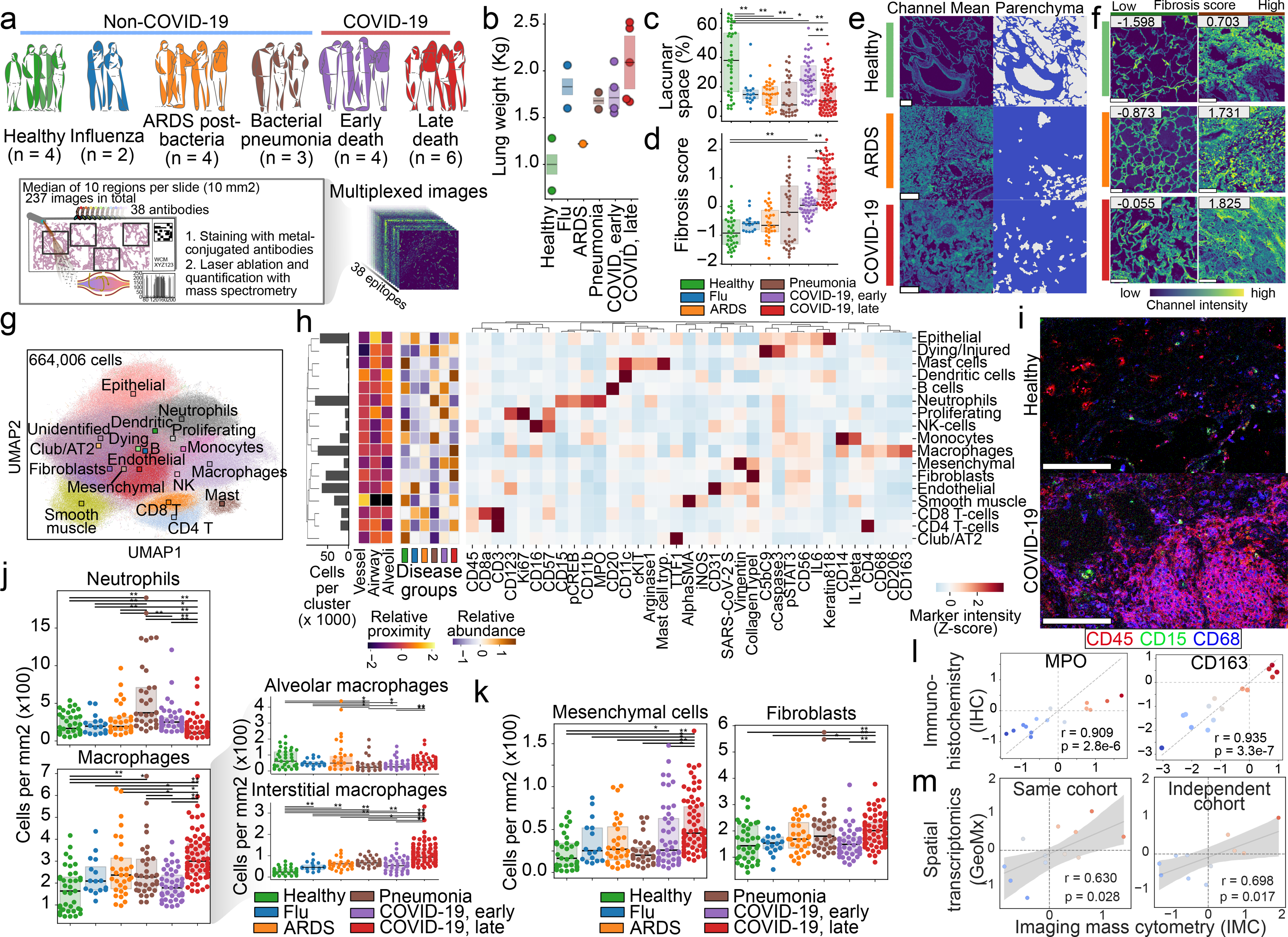
Structural and immunological disorder of lung infection. a, Composition of lung-infection cohort, and schematic procedure to acquire highly multiplexed spatially resolved data with IMC from post-mortem lung samples. b, Total lung weight per disease group measured at autopsy. n = 16 biologically independent samples. c, Lacunar space for each acquired IMC image as a percentage of image area. d, Fibrosis score for each acquired IMC image. e, Representative images illustrating the lacunar and parenchymal structure of healthy lungs, and lungs from patients with ARDS or COVID-19. f, Collagen in images from healthy lungs and lungs from patients with ARDS or COVID-19 and the associated fibrosis score. Images with lowest and highest fibrosis scores are depicted. g, Uniform manifold approximation and projection (UMAP) of all cells, and the metacluster of each cell. Centroids are shown as squares. h, Mean intensity of each marker in each metacluster. Histogram indicates metacluster abundance. Heat maps on left indicate relative proximity to lung structures or abundance per disease group. AT2, alveolar type 2 cells; KRT8/8, KRT8 and KRT18; NK, natural killer. i, Spatial distribution of immune cells in heathy lungs and lungs from a patient with COVID-19. j, Left, abundance of neutrophils (top) and macrophages (bottom) in each disease group. Right, macrophages divided into alveolar (top) and interstitial (bottom) subsets. k, Abundance of mesenchymal cells (left) and fibroblasts (right) in each disease group. l, Amount of change (effect size) pairwise between all disease groups (n = 15) in MPO (left) and CD163 (right) markers between IMC (x axis) and immunohistochemistry (IHC) (y axis). m, Amount of change between late and early COVID-19 groups, pairwise for each cell type (n = 24), as estimated by IMC (x axis) and targeted spatial transcriptomics (y axis) for the same (left) and independent (right) cohorts. For c, d, j, l, m, n, n = 237 images from 27 biologically independent samples. **P < 0.01; *P < 0.05, two-sided Mann–Whitney U test, pairwise between groups, Benjamini–Hochberg false-discovery rate (FDR) adjustment. In o, p, r, Pearson correlation coefficient; P, two-sided P value; shade indicates 95th confidence interval. Scale bars, 100 μm (e, f, k). Box plots show interquartile range (25th to 75th percentiles) with centre line as the median (50th percentile).

Tissue damage by widespread inflammation

Our phenotypic single-cell atlas of the lung contains clusters that are defined by cell-identity markers and markers of cell state across all of the diseases that we evaluated. We developed an unsupervised classification of cells according to the abundance of each marker as a complementary approach (Extended Data Fig. 7a), and observed a high concordance with the phenotypic clusters (Extended Data Fig. 7b). Using this approach, we observed a high specificity of our SARS-CoV-2 S antibody to tissue samples from patients with COVID-19 (Fig. 2a, Extended Data Fig. 7c). Among all cell types, alveolar epithelial cells displayed the highest rate of SARS-CoV-2 S positivity (Fig. 2b). These alveolar epithelial cells were also highly positive for the phosphorylated signal transducer and activator of transcription 3 (pSTAT3), the receptor tyrosine kinase and proto-oncogene KIT and contained increased levels of interleukin 6 (IL-6), arginase 1, the apoptosis marker cleaved caspase 3 (CASP3) and the assembled complement membrane attack complex C5b–C9 (Fig. 2c, d). Given that S− alveolar epithelial cells in the same regions showed no increase in the levels of functional markers, this probably indicates viral-specific alterations of the cellular state. Increased IL-6 and pSTAT3 levels were also seen in the lungs of individuals with influenza and pneumonia as compared with healthy lung, but were not seen in ARDS that was not associated with COVID-19 (Extended Data Fig. 7d). However, high levels of cleaved CASP3 and C5b–C9 were exclusive to S⁺ alveolar epithelial cells from individuals with COVID-19, and indicate the initiation of apoptosis and complement-mediated host immune defence, respectively, which led to increased damage to the alveolar lining. Although the alveolar epithelium was the predominant cell type that was positive for S, we also found that a mean of 7.8% and 2.7% of macrophages and neutrophils, respectively, were positive for S across all images of lungs of patients with COVID-19; some regions were up to 38.6% and 43.6% S⁺, respectively (Extended Data Fig. 7e, f). Consistent with our observations in S⁺ epithelial cells, both macrophages and neutrophils exhibited higher levels of cleaved CASP3, pSTAT3 and IL-6 but—unlike the alveolar epithelial cells—these cells showed no positive staining for C5b–C9 (Extended Data Fig. 7g–j). However, KIT was specifically upregulated in macrophages and not in neutrophils (Extended Data Fig. 7g, h). This non-epithelial cell marker profile phenotype seen in S⁺ cells was also seen in other cell types, albeit at a much lower frequency (Extended Data Fig. 7k). We also observed high heterogeneity in the localization of S⁺ cells, often within the same 1-mm2 tissue region (Fig. 2e). Although we observed interactions between S⁺ epithelial cells and immune and nonimmune cells (Fig. 2e top right), other S⁺ cells did not interact with these cells at all or seemed to be encapsulated in structures that precluded interactions with other cell types (Fig. 2e bottom right). To generate a quantitative map of cellular interactions, we quantified proximal interactions between and within cell types for each image and generated disease-specific interaction maps (Extended Data Fig. 8a–c, Methods). Comparing interactions between the healthy lung and lungs from patients with COVID-19, we observed increased interactions between neutrophils and macrophages and decreased interactions within macrophages; in late COVID-19, the intra-cell-type interactions in macrophages, fibroblasts and CD4⁺ T cells decreased further, and were accompanied by an increase in interactions between macrophages and fibroblasts or dendritic cells (Fig. 2f, g). When spatially contextualizing these interactions, we observed that macrophages preferentially interacted with fibroblasts in the alveolar walls, which suggests a contribution to fibrosis and the thickening of the alveolar wall in late COVID-19 (Fig. 2h). As epithelial cells as a whole did not show any particular change in interactions in the lungs of patients with COVID-19 as compared with healthy lung, we investigated whether S⁺ epithelial cells differed in cellular interactions to their S− counterparts in the lungs of patients with COVID-19 (Extended Data Fig. 8d–i). Across all cell types, there was a trend for S⁺ cells to have reduced cellular interactions (Extended Data Fig. 8d–f). S⁺ alveolar epithelial cells in particular lacked interactions with other cell types, as compared with S− cells (Extended Data Fig. 8g–i). We observed progressively more cells with markers of cell death (particularly macrophages and neutrophils with cleaved CASP3) (Fig. 2i), whereas epithelial and endothelial cells preferentially had C5b–C9 (Fig. 2j, k)—which probably indicates alveolar damage. Using spatial transcriptomics data, we observed that pathways of inflammatory response (such as interferon and interleukin signalling) were increased in the lungs of patients with COVID-19 as compared with healthy lung—particularly in the alveolar and airway compartments in early COVID-19 (Extended Data Fig. 9a–e). However, pathways related to angiogenesis, myogenesis and the epithelial-to-mesenchymal transition were increased in the lungs of individuals with COVID-19 as compared with healthy lungs, which increased progressively in late COVID-19 (Extended Data Fig. 9b). In accordance with the IMC data, we also observed that coagulation, complement activation and apoptosis pathways were upregulated in alveolar areas and in blood vessels in late COVID-19 (Extended Data Fig. 9c). This suggests that, after an early period of disease that is dominated by inflammatory responses to SARS-CoV-2, late COVID-19 in the lung may be driven by pathogen-independent mechanisms that are a consequence of an immune response with an aberrant resolution.

Figure 2:

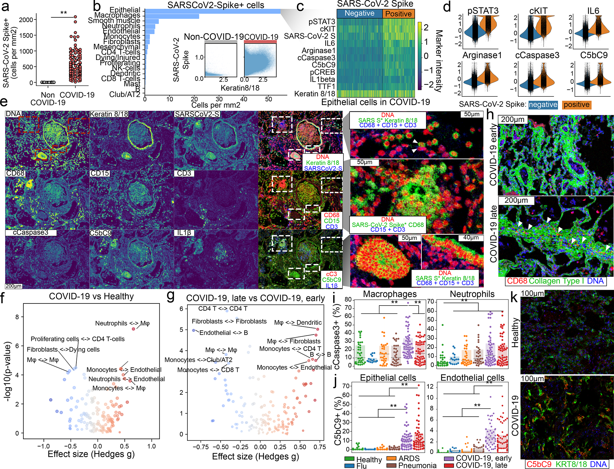
Cellular tropism of SARS-CoV-2 infection. a, Absolute abundance of S+ cells for lungs of patients without COVID-19 (grey) or with COVID-19 (red). b, Distribution of S+ cells across metaclusters in COVID-19. Inset displays intensity of KRT8/18 and S+ for single cells from non-COVID-19 (left) and COVID-19 (right) groups. c, Phenotype of alveolar epithelial cells in COVID-19, depending on levels of S. d, Intensity of differential markers between cells dependent on S levels. e, Distribution of S signal in a spatial context. Structural, cell-type-specific and functional markers are displayed alone or in combination. For the green channel in the images in the rightmost column, the S channel was multiplied with KRT8/18 or CD68 to highlight T cells that are positive for both markers. Scale bar, 200 μm (main panels), 50 μm (magnified images on right (unless otherwise indicated)). f, g, Differential interactions in healthy lung and lungs of patients with COVID-19 (f) or between early and late COVID-19 (g). h, Fibroblasts and macrophages from early and late COVID-19. Scale bars, 200 μm. i, j, Proportion of cleaved CASP3+ macrophages (left) or neutrophils (right) (i), and C5b–C9+ epithelial (left) or endothelial (right) cells (j), for each disease group. k, Deposition of C5b–C9 in epithelial cells in healthy lung and lungs from patients with COVID-19. Scale bars, 100 μm. In a, i, j, n = 237 images from 27 biologically independent samples; **P < 0.01; *P < 0.05, two-sided Mann–Whitney U test, pairwise between groups, Benjamini–Hochberg FDR adjustment. In f, g, P values are from two-sided Mann–Whitney U test with Benjamini–Hochberg FDR adjustment. Box plots show interquartile range (25th–75th percentiles); centre line is median (50th percentile).

An interpretable lanscape of lung pathology

Building on the cell types we identified, their functional status and their interactions, we sought to define a landscape of lung pathology from the data to form an unbiased view of the multicellular architecture of lung tissue during infection (Fig. 3a, Extended Data Fig. 9f–j, Methods; available at http://covid-imc.eipmresearch.org/). The major axes of this landscape, which is based on a principal component analysis, demonstrate the distribution of samples and the major drivers of the establishment of the landscape. This confers biological interpretability to the landscape, as the underlying cellular composition at each given point is readily identifiable. Although the landscape was determined in an unsupervised manner (without knowledge of sample groups), it largely recapitulates the disease ontogeny of the samples: it is dominated by the difference between samples of healthy lung and lungs of patients with COVID-19 who succumbed after prolonged disease (Fig. 3a). This is exemplified by the abundance of immune cell types such as macrophages or neutrophils (which are most abundant in the lungs of patients with COVID-19 or pneumonia, respectively), but also by collagen deposition in lungs from patients with COVID-19 (Fig. 3b). We largely recapitulated the structure of this landscape when using complementary methods (Extended Data Fig. 9h–j). To add a layer of clinical interpretability to the landscape, we performed an association analysis between its axes and known demographic, clinical and pathological factors of patients with lung infections (Fig. 3c, Extended Data Fig. 10a–d, Methods). We observed strong associations primarily between clinical factors and the first principal component (Extended Data Fig. 10a): specifically, a significant positive association between the distribution of samples in the first principal component axis with the presence of alveolar type 2 cells with fibroblasts, organizing pneumonia, the number of days that elapsed since beginning of symptoms, hospitalization and intubation, and lung weight at death (Fig. 3c, Extended Data Fig. 10a). We also observed a significant association between a reduction in white blood cell counts and the major axis associated with disease progression (principal component 1) (Fig. 3c, Extended Data Fig. 10a). The values of clinical factors overlaid with their respective images in the landscape confer a convenient way of interpreting the associations, effectively rendering a landscape annotated with clinical information both biologically (Fig. 3a) and clinically interpretable (Fig. 3d, Extended Data Fig. 10e). To develop the clinical interpretation of the landscape, we further related the associated clinical, demographic and pathological variables by how similar they are in explaining the IMC data (Fig. 3e, Extended Data Fig. 10b). We found that variables were organized into three large blocks: (1) high C-reactive protein and white blood cell count at presentation, as well as pathology characterized by acute inflammation of the alveolar wall; (2) high values of IL-6, erythrocyte sedimentation rate and D-dimer at presentation, comorbidities such as obesity and hypertension, lung pathology characterized by microthrombi and chronic alveolar inflammation with macrophages, and haemorrhagic stroke as the cause of death; and (3) prolonged disease and associated interventions such as intubation and treatment, with pathology characterized by squamous hyperplasia, large thrombi, organizing pneumonia and alveolar type-2 cells associated with fibroblasts. These groups probably represent a progressive range of pathology that is associated with extremely acute disease that results in early death (1) to a chronic manifestation of prolonged disease (3). Beyond these dominant clusters, we found that demographic and behavioural variables (such as age, gender or smoking) did not strongly associate with the larger groups, which suggests they have little influence in the pathology of lethal disease associated with SARS-CoV-2 lung infection. The similarity between variables in the IMC data differs considerably from that obtained from simple co-occurrence of the variables (Extended Data Fig. 10c, d), which provides evidence for the added value of high-content multiplexed imaging of lung tissue in infectious disease.

Figure 3:

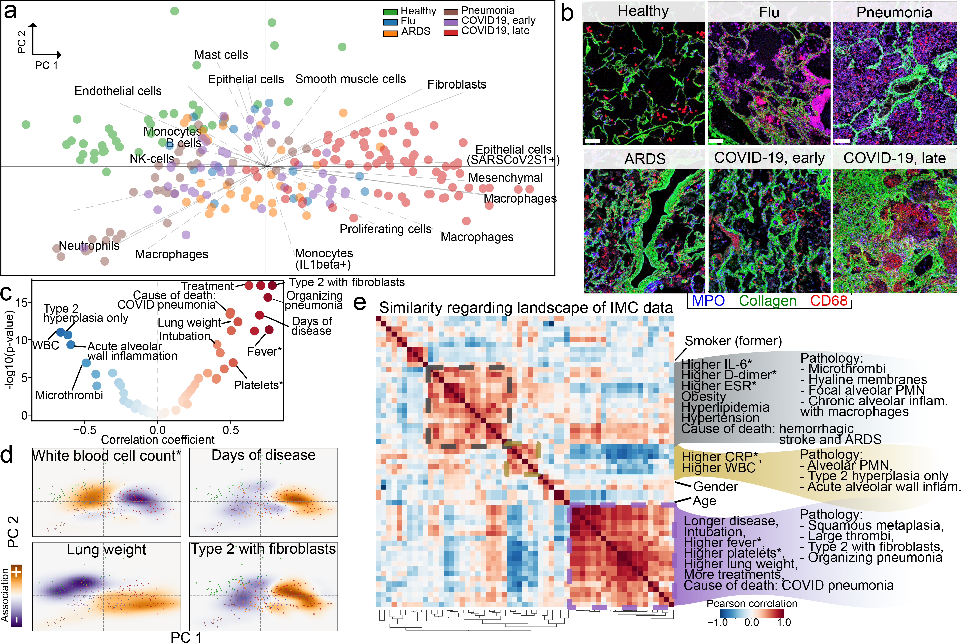
A data-driven and clinically annotated landscape of lung pathology. a, Principal component analysis (PCA) of all IMC images. Points represent images, and are coloured by disease group. Arrows are vectors for each cell cluster, and indicate the area in which each cell type is most abundant. b, Microanatomy and immune content of the disease groups. Scale bar, 100 μm. c, Volcano plot showing strength of association between clinical parameters and principal component (PC)1, and significance. WBC, white blood cell. d, Projections of white blood cell count (measured at admission) (top left), days of disease (top right), lung weight (bottom left) and alveolar type-2 cells with fibroblasts (bottom right) onto the two-dimensional PCA space. e, Similarity of landscape of IMC data. Pairwise correlation of demographic, clinical and pathological variables in the association with the principal components. Matrix rows and columns are the same. Highlighted groups of variables reflect hierarchically clustered groups of variables explaining the IMC data. In c–e, an asterisk indicates that the clinical parameter was measured at admission.

Discussion

Our spatially resolved single-cell analyses of post-mortem lung tissue from patients with COVID-19 or other lung infections provides a comprehensive examination of the response of the human lung to infection, from the macroscopic to the single-cell level. Across all diseases, we observed a significant reduction in alveolar lacunar space, increased immune infiltration and cell death by apoptosis, as compared with healthy lungs. We also noted that neutrophil infiltration—although it is increased in the lungs of patients with ARDS or early COVID-19 compared with normal lung—is a hallmark of bacterial pneumonia, and that a high degree of inflammation, infiltration of interstitial macrophages, complement activation and fibrosis is particular to the lungs of individuals with late COVID-19. Our analysis agrees with recent reports that indicate that the type of pathophysiological response to SARS-CoV-2 infection may not be entirely different from ARDS that is unrelated to COVID-19[14], but contradicts reports that suggest that the hyperinflammatory phenotype (as assessed by cytokine levels in peripheral blood) is not specific to COVID-19[15]. Our observation that S⁺ alveolar epithelial cells do not differentially interact with cells of the immune system (despite extensive immune infiltration in the lung) potentially highlights the lack of an ‘on-target’ immunological response, and the high amount of complement activation in lung tissue from patients with COVID-19 probably results in indiscriminate ‘off-target’ tissue damage—exacerbating COVID-19 and continuing the cycle of inflammation. The increased presence of IL-1β⁺ monocytes in the lungs of patients with early COVID-19 suggests a mechanism for neutrophil recruitment to the lung. Neutrophil recruitment was highest in the lungs of patients with bacterial pneumonia (the only group that we studied with an active disease of bacterial pathogen origin). The differential pathogen recognition between viral and bacterial infection in the lung could explain the differences in chemokine secretion in the ensuing immune response. However, despite sharing a viral pathogenic origin with influenza, COVID-19 (specifically the expansion of mesenchymal cells and fibroblasts, particularly in late COVID-19) probably reflects a response to the extensive tissue damage from complement activation. Despite this, the high mortality rate of COVID-19 is at odds with productive recovery from tissue damage and healing, which suggests the need for further investigation into complement-activation-induced damage to the lung, additional immunological factors (such as neutrophil extracellular traps) and microthrombi formation[19]. This raises the possibility that early immunological interventions that suppress excessive complement activation could have a therapeutic benefit. Our biologically interpretable and clinically annotated landscape of lung pathology provides a framework for a data-driven, spatially aware understanding of lung pathology, and will be an important resource for the study of COVID-19 and other lung infections.

Methods

Data reporting

No statistical methods were used to predetermine sample size. Image acquisition, segmentation, quantification and clustering were blinded to patient identifiers and clinical metadata.

Human studies

Tissue samples were provided by the Weill Cornell Medicine Department of Pathology. The Tissue Procurement Facility operates under Institutional Review Board (IRB) approved protocol and follows guidelines set by Health Insurance Portability and Accountability Act. Experiments using samples from human subjects were conducted in accordance with local regulations and with the approval of the IRB at the Weill Cornell Medicine. The autopsy samples were collected under protocol 20–04021814. Autopsy consent was obtained from the families of the patients.

Tissue section preparation

Lung tissues were fixed via 10% neutral buffered formalin inflation, sectioned and fixed for 24 h before processing and embedding into paraffin blocks. Freshly cut 5-μm sections were mounted onto charged slides.

Antibody panel design and validation

We designed an antibody panel to capture different immune and stromal compartments of the lung. Antibody clones were extensively validated through immunofluorescence and chromogenic staining and verified by a pathologist. Once the clone was approved, 100 μg of purified antibody in BSA and azide free format was procured and conjugated using the MaxPar X8 multimetal labelling kit (Fluidigm) as per the manufacturer’s protocol. To confirm the antibody binding specificity after conjugation and to identify the optimal dilution for each custom conjugated antibody, sections from healthy lung, and bacterial pneumonia, non-COVID-19 ARDS and SARS-CoV-2-infected lung were stained. These sections were then ablated on Fluidigm Hyperion Imaging System and visualized using MCD Viewer for an expected staining pattern and optimal dilution that presented with good signal-to-noise ratio for each channel. For channels with visible spillover into the neighbouring channels, a higher dilution factor was adopted when staining the cohort tissues.

IMC

On the basis of the clinical and pathological characteristics and quality of the preserved tissues, suitable representative fresh cut 4-μm-thick FFPE sections were acquired from the Department of Pathology of Weill Cornell Medicine for IMC staining. The tissues were stored at 4 °C for a day before staining. Slides were first incubated for 1 h at 60 °C on a slide warmer followed by dewaxing in fresh CitriSolv (Decon Labs) twice for 10 min, rehydrated in descending series of 100%, 95%, 80% and 75% ethanol for 5 min each. After 5 min of MilliQ water wash, the slides were treated with antigen retrieval solution (Tris-EDTA pH 9.2) for 30 min at 96 °C. Slides were cooled to room temperature, washed twice in TBS and blocked for 1.5 h in SuperBlock Solution (ThermoFischer), followed by overnight incubation at 4 °C with the prepared antibody cocktail containing all 36 metal-labelled antibodies (Supplementary Table 2). The next day, slides were washed twice in 0.2% Triton X-100 in PBS and twice in TBS. DNA staining was performed using Intercalator-Iridium in PBS solution for 30 min in a humid chamber at room temperature. Slides were washed with MilliQ water and air-dried before ablation.

The instrument was calibrated using a tuning slide to optimize the sensitivity of the detection range. Haematoxylin and eosin-stained slides were used to guide the selection of regions of interest (ROIs) containing alveolar parenchyma, airways and thrombotic vessels to obtain regions that were representative of the whole range of lung pathology. All ablations were performed with a laser frequency of 200 Hz. Tuning was performed intermittently to ensure the signal detection integrity was within the detectable range. A total of 240 image stacks were ablated. The raw MCD files were exported for further downstream processing.

IHC

Automated IHC on a Leica Bond III instrument was performed on 5-μm tissue sections using antibodies for myeloperoxidase (clone 59A5, Leica ready to use antibody, without antigen retrieval) and CD163 (clone MRQ-26, Leica ready to use antibody, antigen retrieval 20 min, high pH) using 3,3′ diaminobenzidine chromogen. For each slide, a grid (5 × 5 grid, 0.4-cm × 0.4-cm boxes) was placed on the section and 5 alveolar, 2 vascular and 2 airway regions were randomly selected using random number-generated x,y coordinates and that ROI (using a 20× objective) was photographed.

Targeted spatial transcriptomics using GeoMx

In brief, selected cases of lung injury associated with COVID-19 (4 patients with early COVID-19 and 4 patients with late COVID-19), bacterial pneumonia (2) and healthy lung (3) from the IMC cohort were evaluated using the GeoMx[24] COVID-19 Immune Response Atlas with approximately 1,850 RNA targets. Spatial transcriptomics analysis included up to 24 ROIs per tissue. Alveolar, airway and vascular compartments were analysed.

For GeoMx DSP slide preparation, we followed the GeoMx DSP slide preparation user manual (MAN-10087–04). In brief, tissue slides were baked in a drying oven at 60 °C for 1 h and then loaded to Leica Biosystems BOND RX FFPE for deparaffinization and rehydration. After the target retrieval step, tissues were treated with proteinase K solution to expose RNA targets followed by fixation with 10% NBF. After all tissue pretreatments were done, tissue slides were unloaded from the Leica Biosystems BOND RX and incubated overnight with RNA probe mix (COVID-19 Immune Response Atlas; a pool of in situ hybridization probes with UV photocleavable oligonucleotide barcodes). The next day, tissues were washed and stained with tissue visualization markers: CD68–647 at 1:400 (Novus Bio, NBP2–34736AF647), CD45–594 at 1:10 (NanoString Technologies), panCK-532 at 1:20 (NanoString Technologies) and/or SYTO 13 at 1:10 (Thermo Scientific S7575).

For GeoMx DSP sample collections, we followed the GeoMx DSP instrument user manual (MAN-10088–03). In brief, tissue slides were loaded on the GeoMx DSP instrument and then scanned to visualize whole-tissue images. For each tissue sample, a board-certified pathologist selected 24 total ROIs from 3 types of functional tissue: vascular zone, large airway and alveoli zone. Each ROI was subdivided into compartments on the basis of fluorescent cell-specific markers, and serial UV illumination of each compartment was used to sequentially collect the probe barcodes from the different cell types.

Each GeoMx DSP sample plus nontemplate controls (NTCs) was uniquely indexed using the i5 × i7 dual-indexing system of Illumina. Four μl of a GeoMx DSP sample was used in a PCR reaction with 1 μM of i5 primer, 1 μM i7 primer and 1× NSTG PCR Master Mix. Thermocycler conditions were 37 °C for 30 min, 50 °C for 10 min, 95 °C for 3 min, 18 cycles of 95 °C for 15 s, 65 °C for 60 s, 68 °C for 30 s, and final extension of 68 °C for 5 min. PCR reactions were purified with two rounds of AMPure XP beads (Beckman Coulter) at 1.2× bead-to-sample ratio. Libraries were paired-end sequenced (2 × 75) on a NextSeq550 generating up to 400 million aligned reads in total.

Processing and filtering of the raw next-generation sequencing data was performed on the DNA sample libraries that were sequenced, producing about 1.3 billion reads. NextSeq-derived FASTQ files for each sample were compiled for each compartment using the bcl2fastq program of Illumina, and then demultiplexed and converted to digital count conversion (DCC) files using the GeoMx DnD pipeline (v.1) of Nanostring. These DCC files were then converted to an expression count matrix using a custom Python script. A minimum of 10,000 reads were required for each non-NTC sample (2 compartments removed). Probes were checked for outlier status by implementing a global Grubb’s outlier test with alpha set to 0.01. The counts for all remaining probes for a given target were then collapsed into a single metric by taking the geometric mean of probe counts. A count of 1 was added to any probe that yielded 0 counts before the geometric mean was taken. For each sample, an RNA-probe-pool-specific negative probe normalization factor was generated on the basis of the geometric mean of negative probes in each pool. To ensure good data quality, we calculated the 75th percentile of the gene counts (that is, geometric mean across all nonoutlier probes for a given gene) for each ROI, and normalized to the geometric mean of the 75th percentile across all ROIs to give the upper quartile (Q3) normalization factors for each ROI. The distribution of these Q3 normalization factors were then checked for outliers defined as any ROI greater than two s.d. from the mean log2-transformed Q3 normalization factor. This criterion removed 15 ROIs that fell below the range and 1 ROI that fell above the range.

Preprocessing IMC data

IMC data were preprocessed as previously described[26] with some modifications. In brief, image data were extracted from MCD files acquired with the Fluidigm Hyperion instrument. Hot pixels were removed using a fixed threshold, the image was amplified two times, Gaussian smoothing was applied and, from each image, a square 500-pixel crop was saved as a HDF5 file for image segmentation. Segmentation of cells in the image was performed with ilastik[27] (version 1.3.3) by manually labelling pixels as belonging to one of three classes: nuclei (the area marked by signal in the DNA and histone H3 channels), cytoplasm (the area immediately surrounding the nuclei and overlapping with signal in cytoplasmic channels) and background (pixels with low signal across all channels). Ilastik uses the labelled pixels to train a random forest classifier using features derived from the image and its derivatives. Features used were the Laplacian of the Gaussian, Gaussian gradient magnitude, difference of Gaussians, structure tensor eigenvalues and the Hessian of Gaussian eigenvalues, each of which had Gaussian kernels of widths from 0.3 to 10 (37 features in total). The outputs of prediction are class probabilities for each pixel, which were used to segment the image using CellProfiler[28] (version 3.1.8) with the IdentifyPrimaryObjects module. This was followed by the IdentifySecondaryObjects module, in which the identified nuclei are used to seed an expansion of the cell area to the area with the sum of the nuclear and cytoplasmatic probability map, and finally gaps in the identified cells are filled.

We assessed the quality of each acquired channel by computing a set of metrics for each channel across all images: the mean and squared coefficient of variation of each channel in the whole image and, in the area with cells, a difference between those values in the cells and the whole image (foreground versus background signal), an estimate of noise variance[29], a robust wavelet-based estimator of Gaussian noise s.d.[29,30], the fractal dimension (Minkowski–Bouligand approximation using the box counting method) and lacunarity of the image[31]. Across all 240 ablated images three were discarded based on these metrics and visual inspection.

Computing lacunarity and fibrosis score

To identify lacunae in the images, we used the mean of all channels in each image stack after performing histogram equalization per channel (skimage.exposure.equalize_hist). Images were thresholded with Otsu’s method (skimage.filters.threshold_otsu), successively dilated and closed (ski.morphology.binary_dilation/ski.morphology.closing) with a disk of 5-μm diameter to remove objects without holes and—for the objects with holes—objects within the hole were removed on the negative image (scipy.ndimage.binary_fill_holes) and only objects with area larger than 625 pixels (252) were kept (skimage.morphology.remove_small_objects). To provide biological context for the single-cell clusters we identified, we further classified each of the lacuna of healthy lungs into one of three classes: blood vessels (arteries and veins), airways and alveoli. Vessels showed a very thin lining of endothelial cells, followed by a thick layer of smooth muscle cells that are α-SMA⁺; the airway epithelium is lined by KRT8⁺KRT18⁺ cells; and alveoli are covered in alveolar epithelial cells that have various degrees of CD31, vimentin, KRT8 and KRT18. On the basis of this, we developed a semisupervised strategy for lacuna classification that had two stages: first each of the lacuna objects was dilated by a 15-pixel disk and the mean intensity of the channels above was quantified only in the dilated area, and these values were Z-score-transformed per image. We used these values in three ways, in which each provided a vote towards a lacuna being one of the three classes: absolute intensity, Z-score-transformed intensity, ratio of α-SMA to KRT8 and KRT18. For each, a set of rules was enforced in which lacunae with higher values in α-SMA and low in KRT8 and KRT18 were labelled as vessels, and those with higher KRT8 and KRT18 were labelled as airways; the remaining lacunae were labelled as alveoli. Essentially, absolute and relative intensity of the markers determine the class, and the ratio of the two is the tiebreaker in case of disagreement. In a second phase, the suggested labels were reviewed by an expert and overruled if needed. In general, we found that the rules above were accurate with only a systematic bias to underclassify vessels (hence the need for supervision).

To develop a score for fibrosis, we were inspired by the Ashcroft score[23] in which the fraction of fibrotic tissue that occupies each image is translated into a score in a Likert scale. We quantified the fraction of the image occupied by collagen type I as thresholded by the Otsu method (skimage.filters.threshold_otsu), but in addition quantified the density of collagen per area unit by using the spectral counts given by the IMC data. The final score is the mean of a Z-score of the fraction covered by collagen and a Z-score of its intensity.

Cell-type identification

To identify cell types in an unsupervised fashion, we first quantified the intensity of each channel in each segmented cell that did not overlap image borders. In addition, for each cell we computed the morphological features ‘area’, ‘perimeter’, ‘major_axis_length’, ‘eccentricity’ and ‘solidity’ (skimage.measure.regionprops_table). Values were Z-scored per image and cells with area values above −1.5, solidity above −1 and eccentricity below 1 were kept. In addition, we calculated the sum of log(1 + x) signals in the IMC channels and kept cells with values between 2 and 7. We used Scanpy[32] (version 1.6.0) to perform a PCA, compute a neighbour graph on the PCA latent space, compute a UMAP[10] embedding (umap package, version 0.4.6) and cluster the cells with the Leiden algorithm[33] with resolution 1.0 (leidenalg package, version 0.8.1). Each cluster was manually labelled with a broad ontogeny and the channels that were most abundant in each cluster. These broad labels formed the basis of the metaclusters used to aggregate clusters on the basis of cell type and regardless of cellular state. Clusters without enrichment for any particular marker were not aggregated.

To obtain an easy way to quantify the fraction of cells positive for a given marker, we used univariate Gaussian mixture models using scikit-learn[34] (version 0.23.0). For each channel, we performed model selection with models with two to six mixtures, selected the model on the basis of the Davies–Bouldin index[35] and labelled a cell as positive for a given channel if its value was in the top mixture (in cases in which the selected model had only two mixtures) or the top two mixtures (if the selected model had more). The analysis of the immune-centric IMC panel was performed in the same manner as the larger dataset, with the exception that the thresholds for cell filtering based on area, DNA intercalator intensity and solidity were performed automatically with Gaussian mixture models as described in the previous paragraph. Differential marker abundance was tested with a two-sided Wald test between healthy lung samples and samples from patients with COVID-19, and adjusted for multiple comparisons with the Benjamini–Hochberg FDR.

Quantification of cellular interactions

To quantify the degree and importance of intra- and inter-cell-type interactions, we started by constructing a region adjacency graph representing the interactions between cells, in which the edges are weighted by the Euclidean distances between cells, using scikit-image[36] (version 0.17.2). A pairwise adjacency matrix between cell clusters was computed using networkx[37] (version 2.5). To get a degree of confidence on cellular interactions given the cell type abundance in each image, we permuted the cell cluster assignments 1,000 times and computed the difference between the log-normalized frequency of cell-type interactions in the real data versus the permuted (interaction scores). For visualization, we generated chord plots by aggregating the interaction scores of the images from each disease group or subgroups by the fraction of images with an interaction score was higher than 1. To discover differential interactions specific to a subgroup, we tested whether the distribution of interaction scores between disease groups or subgroups for each pairwise cell-type combination was different as described in ‘Analysis of IHC data’.

Analysis of IHC data

IHC images were segmented with Stardist[38] (version 0.6.1) with the 2D_versatile_he pretrained model and normalization to the unit space after capping the intensity to the 3rd and 98th percentiles. The image was decomposed into a haematoxylin and diaminobenzidine intensity channels using a preset colour space for the stains from the scikit-image package[36] (skimage.colour.hdx_from_rgb) and the intensity of each nuclei in both channels was calculated by a mean reduction. As the H-DAB and IHC signal in general does not linearly reflect the molecular stoichiometry of chemical reactions, we discretized the signal into positive and negative fractions per image by using Gaussian mixture models with model selection in the same way as for the IMC data. Cells were declared positive for a stain if they belonged to the group with highest signal. For the quantification of image lacunarity in IHC data we first normalized illumination in YCrCb colour space by applying a Gaussian blur with 5 pixels of s.d. per 300 × 300 size image and subtracting this background from the brightness channel (Y or luma). Images were converted back to RGB colour space and the inverted mean of the channels was segmented using the Otsu method. The lacunarity of the image is the fraction of the image covered in background. This was performed only for MPO-stained images within the alveolar space and not with airways or vessels.

Analysis of targeted spatial transcriptomics data using GeoMx

To transform the gene set space into a cell-type space that would be compatible with the cell types identified in the IMC dataset, we performed single-sample gene set enrichment analysis (ssGSEA) using GSEAPY (version 0.10.2). For each ROI, gene set signatures used were from the molecular signatures database (MSigDB, version 7.2); in particular, the cell-type signature gene sets (group C8) were used. ssGSEA enrichment values were Z-scored, and signatures containing the keywords ‘Epithelial’, ‘Mesenchym’, ‘Fibroblast’, ‘Smooth_muscle’, ‘Club’, ‘CD4_T’, ‘CD8_T’, ‘NK_cell’, ‘Macrophage’, ‘Monocyte’, ‘Neutrophil’, ‘B_cell’, ‘Mast’ and ‘Dendritic’ were grouped and averaged, generating an enrichment score for each ROI in each cell type. If a group was composed of less than three signatures it was discarded. For the pathway-based functional analysis of lung tissue, ssGSEA was performed on the Hallmark group of gene set signatures from MSigDB (group H) without further aggregation.

PCA of lung pathology and association with clinical parameters

To create the unsupervised landscape of lung pathology, we used PCA on a matrix of cell counts per cell cluster (features) and per image (observations), after previous normalization by total, scaling and centring, using the Scanpy implementation. The feature loadings were plotted on the same dimensions as the observations by scaling them by a constant factor of 20. The correlation coefficient between each principal component and the continuous clinical variables was used as a relative measure of direction and strength of association. However, the significance of association was assessed by permuting the clinical variables 106 times and using the mean and s.d. of the correlation coefficients from the permuted data as location and scale parameters, respectively, of a normal distribution, from which the 2 × CDF(|x|) was calculated as a two-tailed empirical P value. All principal components and clinical factors were permuted and the empirical P values were adjusted with the Benjamini–Hochberg FDR method. We used the signed empirical, FDR-corrected P values as an effectively regularized measure of association between principal components and clinical factors. To project the clinical parameters into the PCA space, we fit Gaussian kernel density estimator functions to the distribution of the images in the first principal components, in one case without and another with the numeric values of the clinical variables as weights. The difference in predicted densities in the two-dimensional space between the weighted and unweighted kernels was used as a visual aid to identify regions in the latent space with relatively higher or lower fraction of samples with that clinical parameter.

Statistics and reproducibility

Unless otherwise stated in the figure legends, statistical testing was performed pairwise between groups with a two-sided Mann–Whitney U test, and adjusted for multiple comparisons with the Benjamini–Hochberg FDR method using pingouin[39] (version 0.3.7). Estimated values of central tendency, effect sizes and P values are provided in Supplementary Tables 3, 4. In the box plots in all figures, the box is the interquartile range (25th to 75th percentiles) and the centre line is the median (50th percentile). Experiments were not repeated independently, owing to the use of unique autopsy material.

The following software versions were used: Python, version 3.8.2; numpy[40], version 1.18.5; scipy[41], version 1.4.1; scikit-image[36], version 0.17.2; networkx[37], version 2.5; Scanpy, version 1.6.0; pingouin[39], version 0.3.7; CellProfiler[28], version 3.1.8; and Stardist[38], version 0.6.1.

Extended Data

Extended Data 1:

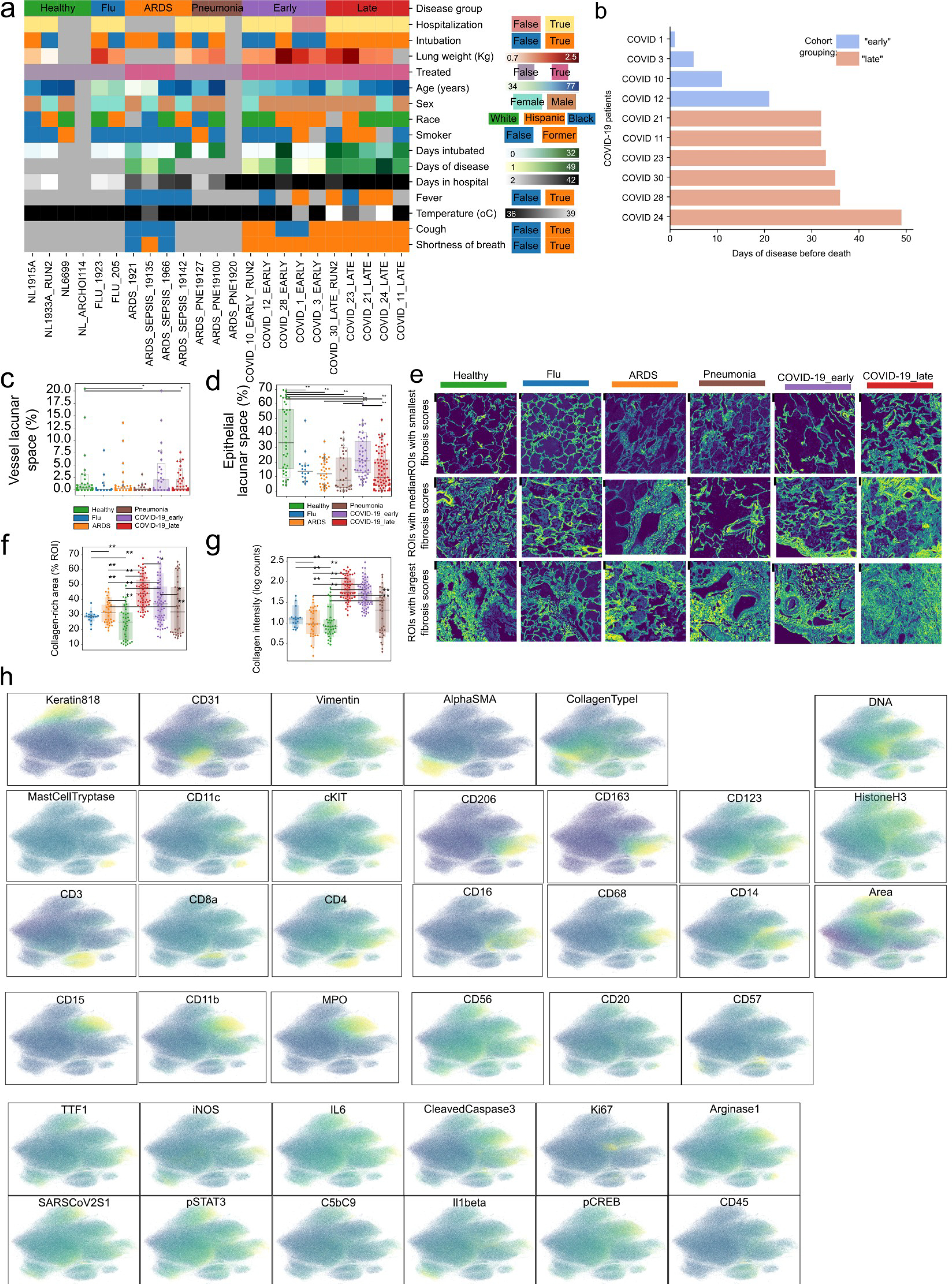
a) Heatmap depicting the values of each individual for all acquired clinical and demographic variables. Grey color indicates missing or non-applicable values. b) Time of death relative to start of symptoms in COVID-19 patients. c-d) Percentage of lacunar space attributed to a) vessel or b) epithelial space per image grouped by disease. e) Collagen type I in images from lungs of healthy individuals, or lung pathology patients and the associated fibrosis score. Images with lowest, median and highest fibrosis scores are depicted. f) Percentage of image covered in Collagen type I for each image grouped by disease group. g) Mean intensity of Collagen type I in lung IMC images grouped by disease group. h) UMAP projection of all single-cells where cells are colored by the intensity of each channel. For panels c), d), f), and g): ** p < 0.01; * p < 0.05, two-sided Mann-Whitney U-test, pairwise between groups, Benjamini-Hochberg FDR adjustment.

Extended Data 2:

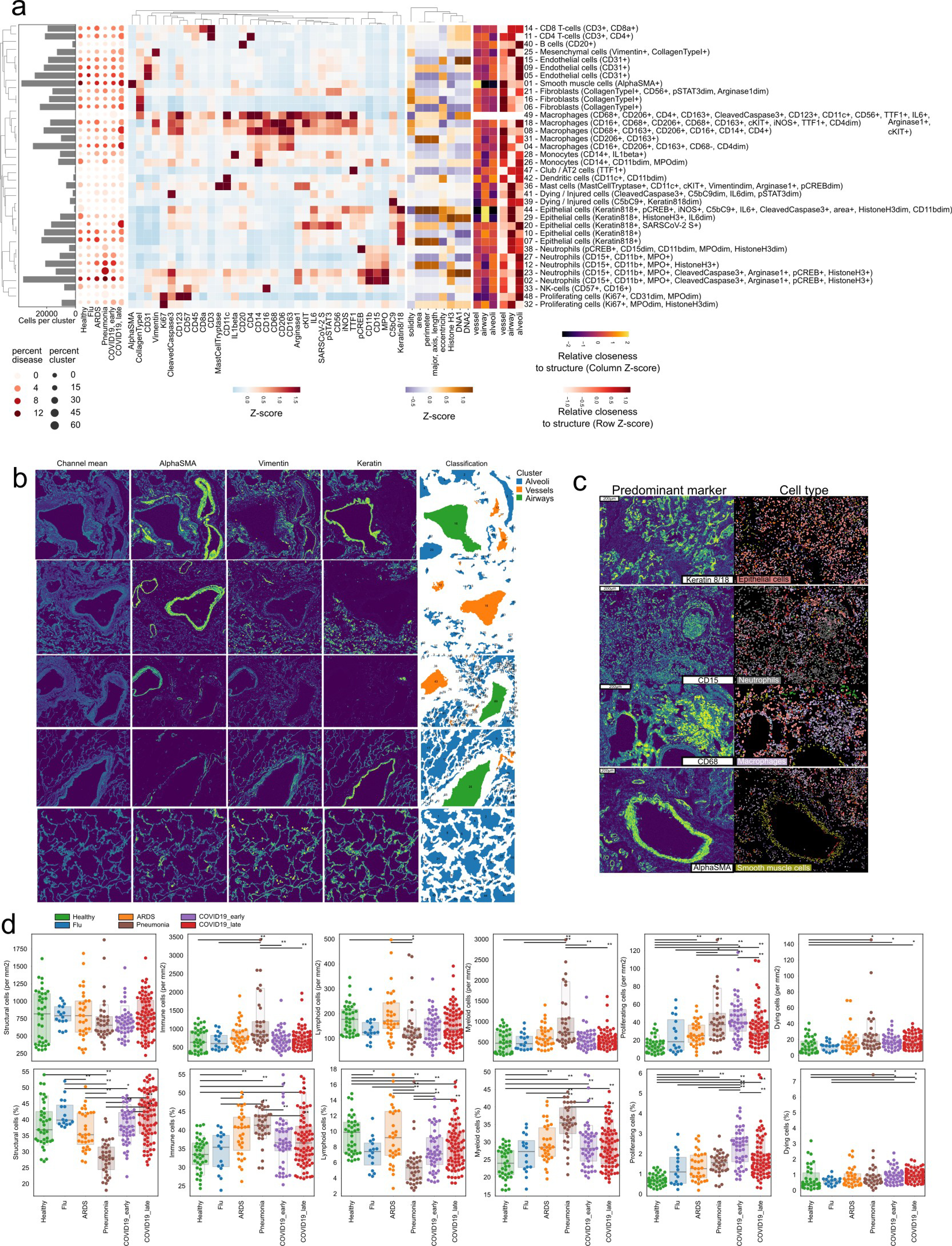
a) Hierarchically clustered heatmap of discovered clusters (rows) and the mean intensity of each channel (columns) for each. The histogram on the left represents the absolute abundance of each cluster across all images. The dot-plot represents the relative abundance of each cluster in each disease group. b) Classification of lung lacunae. Representative images of healthy lung images with the mean of all channels and channels important to discern between vessels, airways and alveoli. The last column represents the final classification of lacunae into each of the three classes of structures. c) Representative spatial context of three meta-clusters (rows). The column on the left displays the spatial distribution of the most predominant marker for each meta-cluster, while the column on the right represents segmented cells colored by the meta-cluster they were assigned to. d) Global abundance of structural and immune cells. Absolute (first row) and relative (second row) abundance of groups of cells dependent on disease group. ** p < 0.01; * p <0.05, two-sided Mann-Whitney U-test, pairwise between groups, Benjamini-Hochberg FDR adjustment.

Extended Data 3:

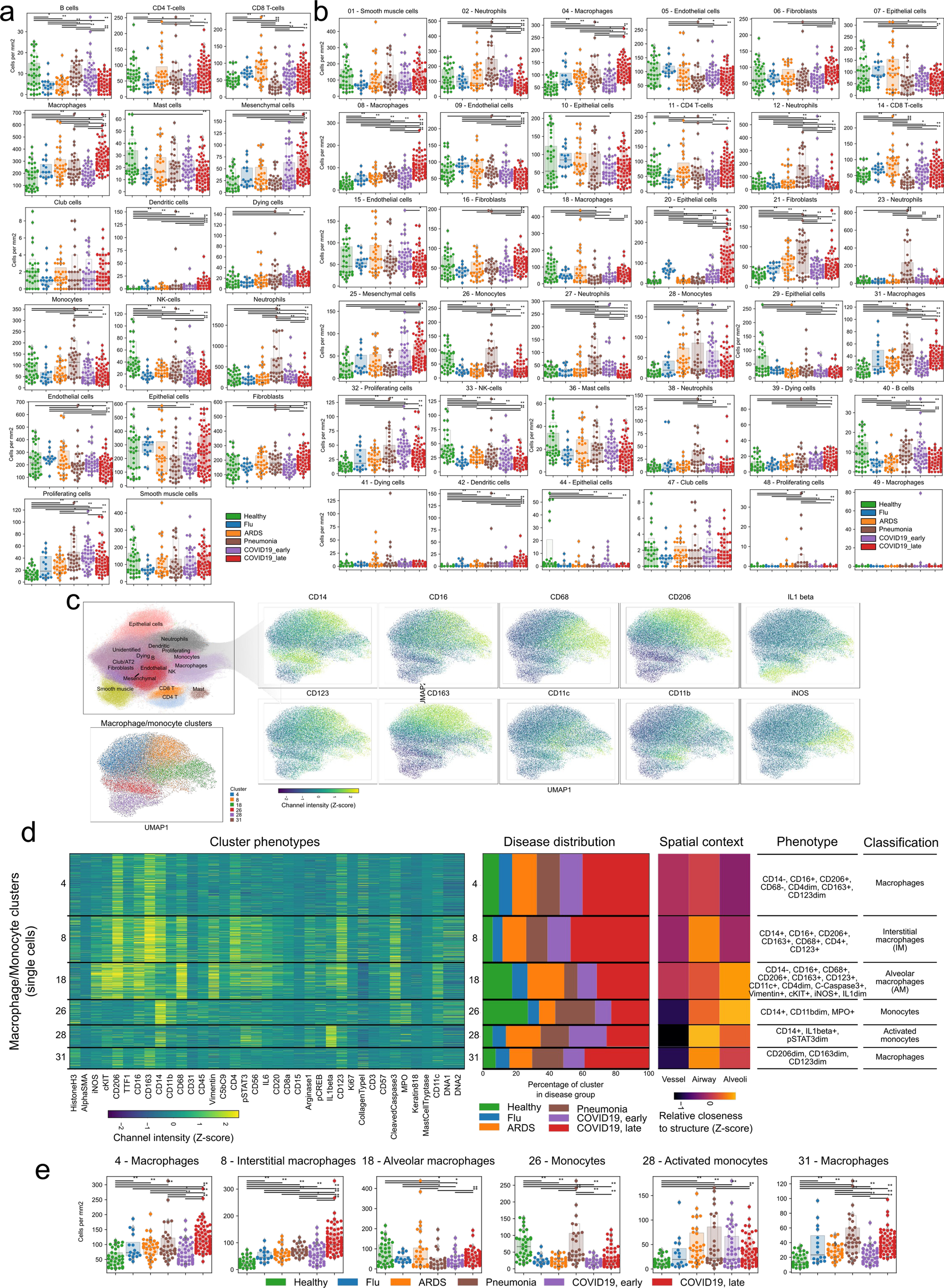
a-b) Absolute abundance of a) meta-clusters or b) clusters per image, grouped by disease group. c-e) Diversity of myeloid cells in the lung. c) UMAP representation of myeloid cells and the prominent markers associated with them. d) Phenotypic markers, spatial context and abundance in disease groups for each of the 6 myeloid clusters. e) Abundance of each myeloid cluster in the disease groups. Each point represents the abundance of that cluster in a given region of interest. For panels a), b), and e): ** p < 0.01; * p < 0.05, two-sided Mann-Whitney U-test, pairwise between groups, Benjamini-Hochberg FDR adjustment.

Extended Data 4:

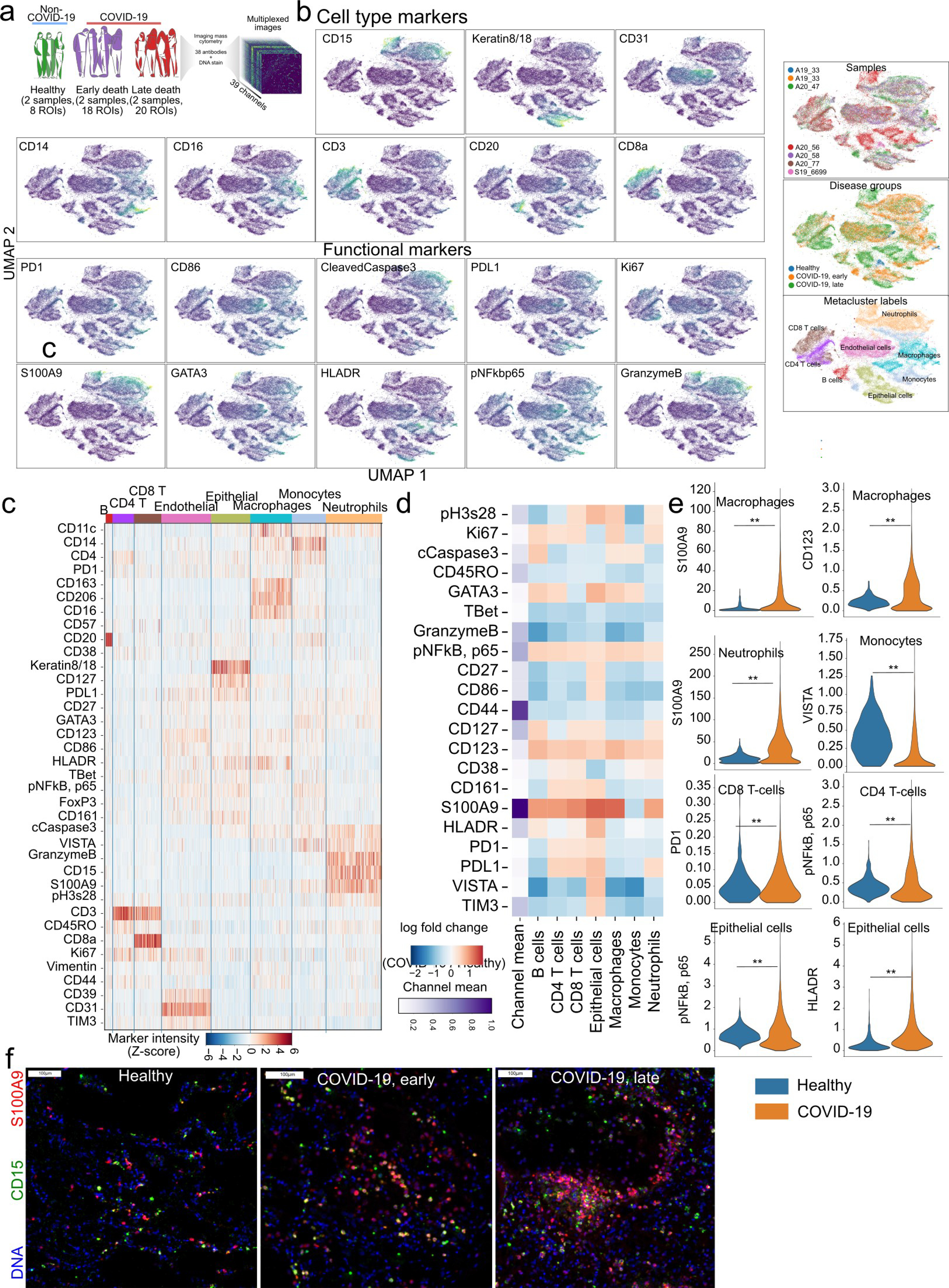
a) Schematic experimental design of new IMC panel and its application to healthy and COVID-19 lung tissue samples. b) UMAP representation of single-cells coloured by the intensity of the marker for cell-type defining markers and functional markers. c) Expresion of markers for each single-cell grouped by the cell type. d) Differential expression of functional markers between COVID-19 and Healthy lung for each cell type. e) Expression range represented as violinplots for the selected cell types from b), between COVID-19 and healthy lung. ** p < 0.01 two-sided Wald test, Benjamini-Hochberg FDR adjustment. f) Representative images of S100A9 and CD15 marker expression in Healthy lung and COVID-19. All scale bars represent 100 microns.

Extended Data 5:

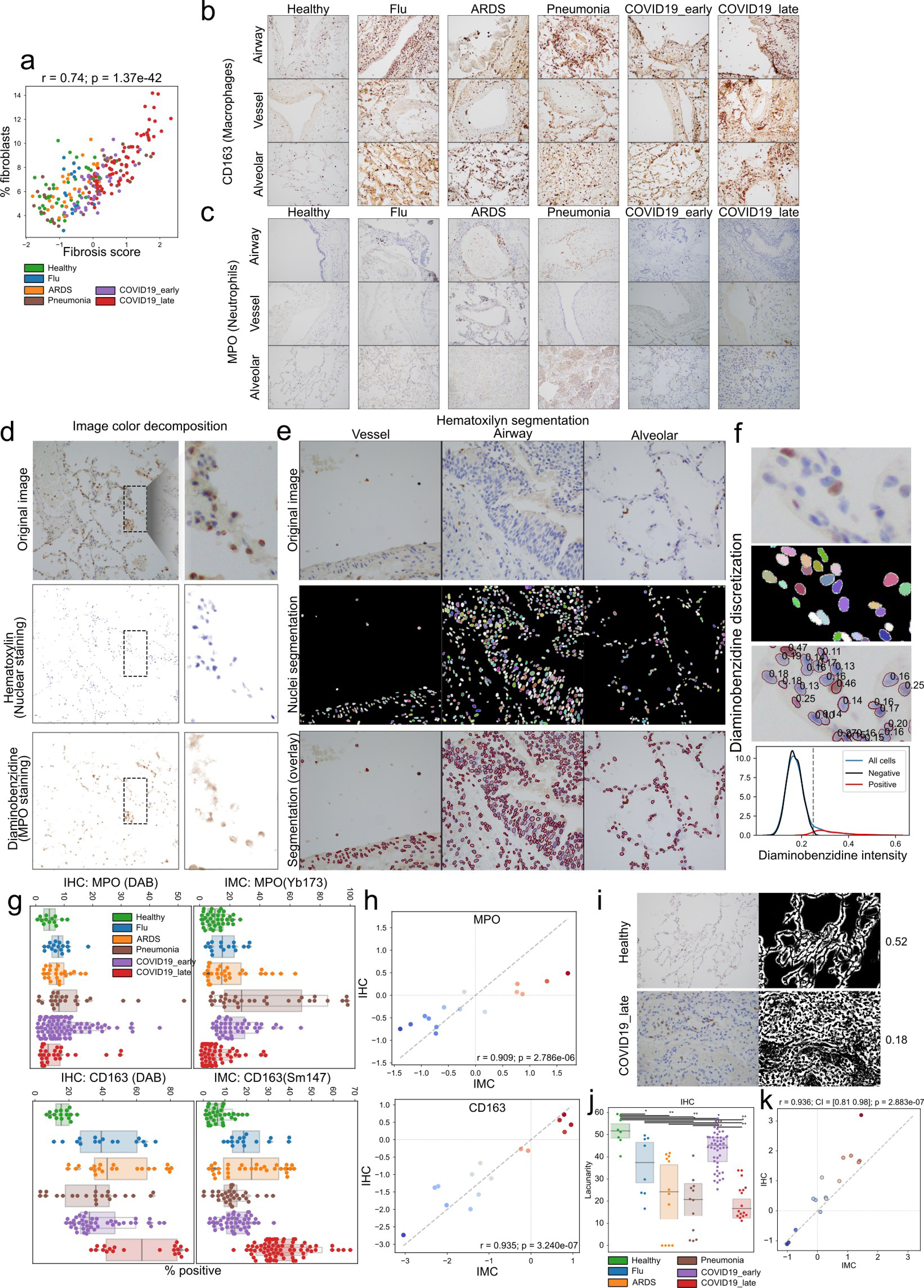
a) Relationship between fibrosis score and fibroblast meta-cluster abundance visualized as a scatter plot. b-c) Immunohistochemistry for two markers across all disease groups. Hematoxylin-diaminobenzidine staining of b) CD163 or c) MPO in tissue from healthy and diseased lung matching the patients in the IMC cohort. d) Analysis of immunohistochemistry data. Example images demonstrating the process of color decomposition underlying the separation of the hematoxylin (nuclei) and diaminobenzidine (either CD163 or MPO) (H-DAB) in lung tissues. e) Example images demonstrating the process of nuclei segmentation employed. The left column shows the original images in RGB space, the middle the resulting segmentation where each nuclei has a random color and the background is black, and the right column which overlays the borders of segmented nuclei in red over the original image. f) Example image section demonstrating the process of quantification of diaminobenzidine stain. The first panel shows the original image in RGB space, the second the nuclei segmentation, the thid the numeric value of the DAB stain for each nuclei, and the fourth a histogram of nuclei intensity in DAB stain modeled as a Gaussian mixture with two components used to discretize nuclei into negative or positive for DAB based on a threshold which best separates the two mixtures. g) Percentage of cells within an image which is positive for the respective DAB stain in IHC (left columns) or positive for the respective marker in IMC data (right column). h) Comparison of the estimated effect sizes of change between disease groups estimated from IMC data (x-axis) or IHC (y-axis) for the two stains. The Pearson correlation coefficient and its significance are indicated. i) Analysis of image lacunarity with IHC data. Representative images of lacunarity for healthy and late COVID-19 immunohistochemistry data. For each image the original image and the segmented background space is shown along with the lacunarity value for the image which is the fraction of the image without cells which represents the alveolar/capillary space. j) Quantification of lacunarity across MPO images in IHC. ** p < 0.01; * p < 0.05, two-sided Mann-Whitney U-test, pairwise between groups, Benjamini-Hochberg FDR adjustment. k) Comparison of the estimated effect sizes of change in lacunarity between disease groups estimated from IMC data (x-axis) or IHC (y-axis). For panels a), h), and k): r = Pearson coeffcient; p = its two-tailed p-value.

Extended Data 6:

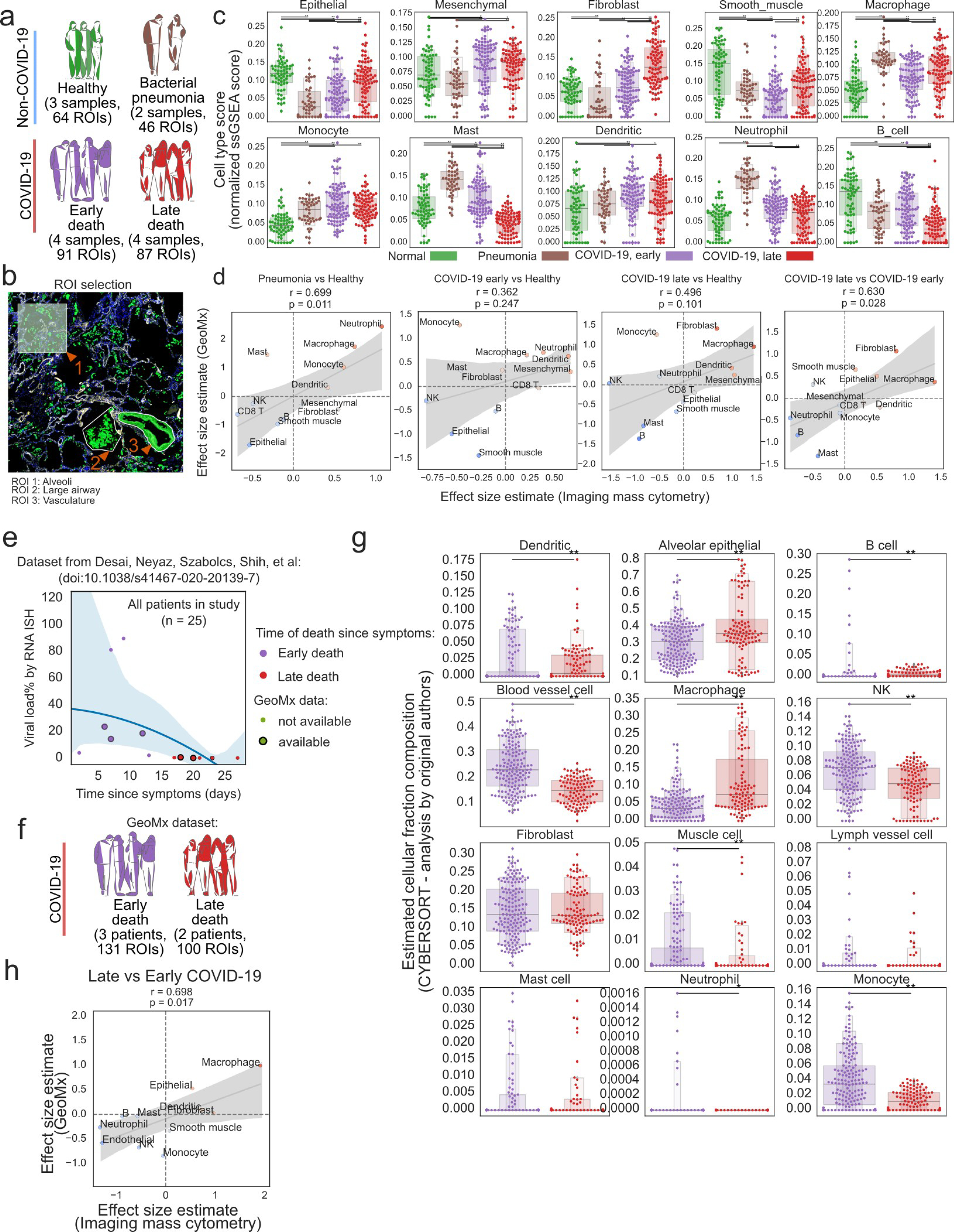
Profiling of lung tissue with targeted spatial transcriptomics (GeoMx). a) Experimental design of GeoMx dataset. b) Representation of the procedure to choose regions of interest within the lung tissue to capture with GeoMx. c) Enrichment of cell type-specific gene set signatures for various cell types matching IMC across disease groups. d) Comparison of the estimated changes in cell type abundance with IMC (x-axis) and gene set signatures in GeoMx (y-axis). e) Viral load dependent on the time of death since beginning of COVID-19 symptoms in an independent cohort. COVID-19 samples were categorized into “early” or “late” death depending if death occurred before or after 15 days respectively. f) Schematic representation of the cohort of patients for which GeoMx data is available: in total 5 pateints and 231 ROIs. g) Estimated fractions of cell type composition by the CYBERSORT program between early and late COVID-19 death from the original publication. h) Comparison of the estimated changes in cell type abundance with IMC (x-axis) and GeoMx (y-axis) between late and early COVID-19 death. For panels d) and h): r = Pearson coefficient, p = its two tailed p-value; shaded area indicates 95th confidence interval. For panels c) and g): ** p < 0.01; * p < 0.05, two-sided Mann-Whitney U-test, pairwise between groups, Benjamini-Hochberg FDR adjustment.

Extended Data 7:

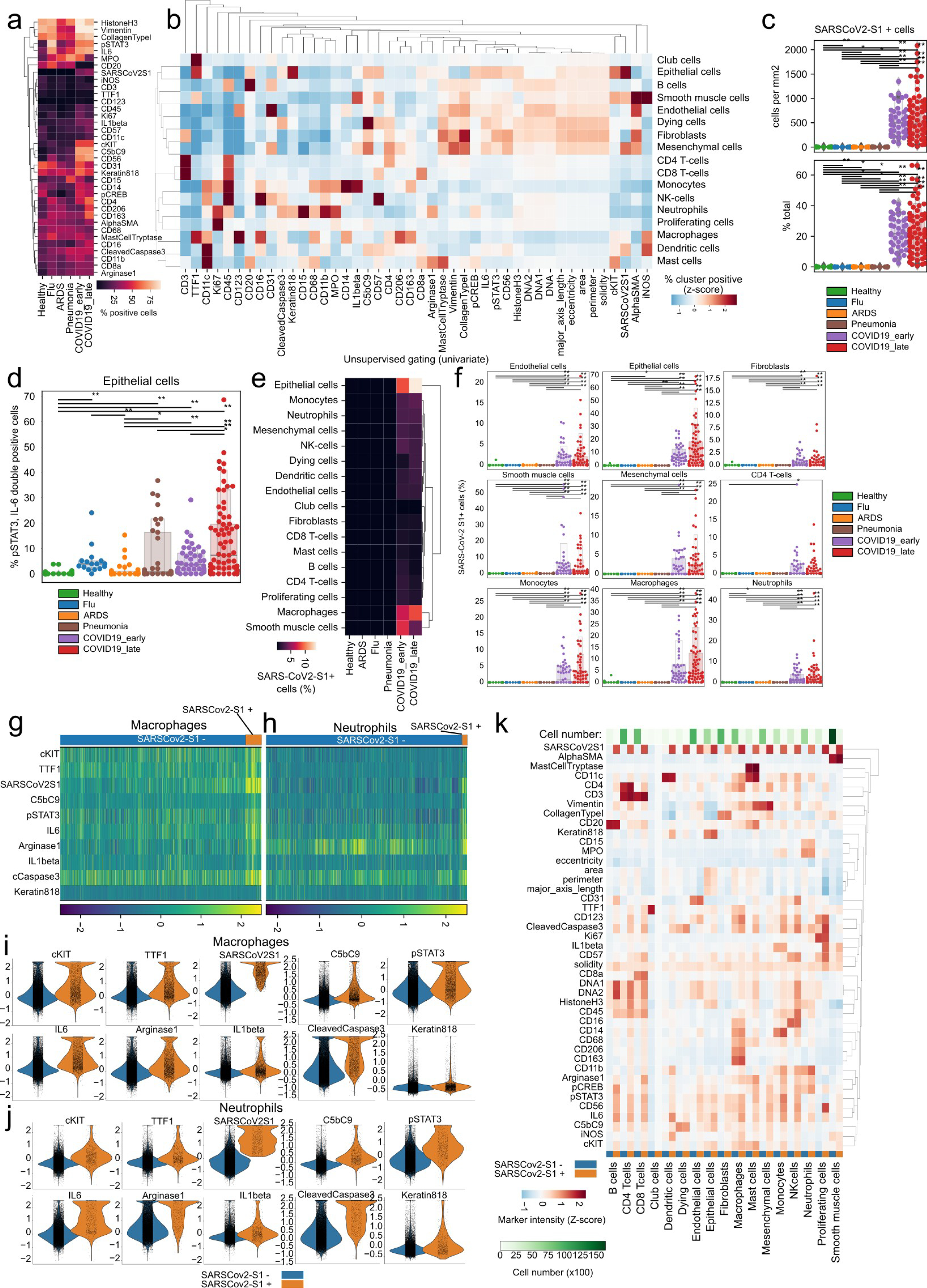
a) Percentage of cells positive for each IMC channel as classified by univariate Gaussian mixture models per disease group. b) Percentage of channel positive cells per each meta-cluster. Values represent a column-wise Z-score. c) Absolute (top) and relative (bottom) frequency of SARS-CoV-2 Spike+ cells per disease group. d) Proportional abundance of SARS-CoV-2 Spike+, IL6+, pSTAT3+ cells across disease groups. e) Proportional amount of SARS-CoV-2 Spike+ cells grouped per meta-cluster and disease group. f) Proportional frequencies of cells positive for SARS-CoV-2 Spike+ cells per meta-cluster and disease group. g-h) Heatmap of single g) macrophage or neutrophils h) (columns) and functional markers (rows) with cells grouped by SARS-CoV-2 Spike positivity. i-j) Intensity of IMC channels per single-cell dependent on SARS-CoV-2 Spike positivity for i) macrophages and j) neutrophils. k) Mean channel intensity for all metaclusters dependent on SARS-CoV-2 Spike positivity. For panels c), d), and f): ** p < 0.01; * p < 0.05, two-sided Mann-Whitney U-test, pairwise between groups, Benjamini-Hochberg FDR adjustment.

Extended Data 8:

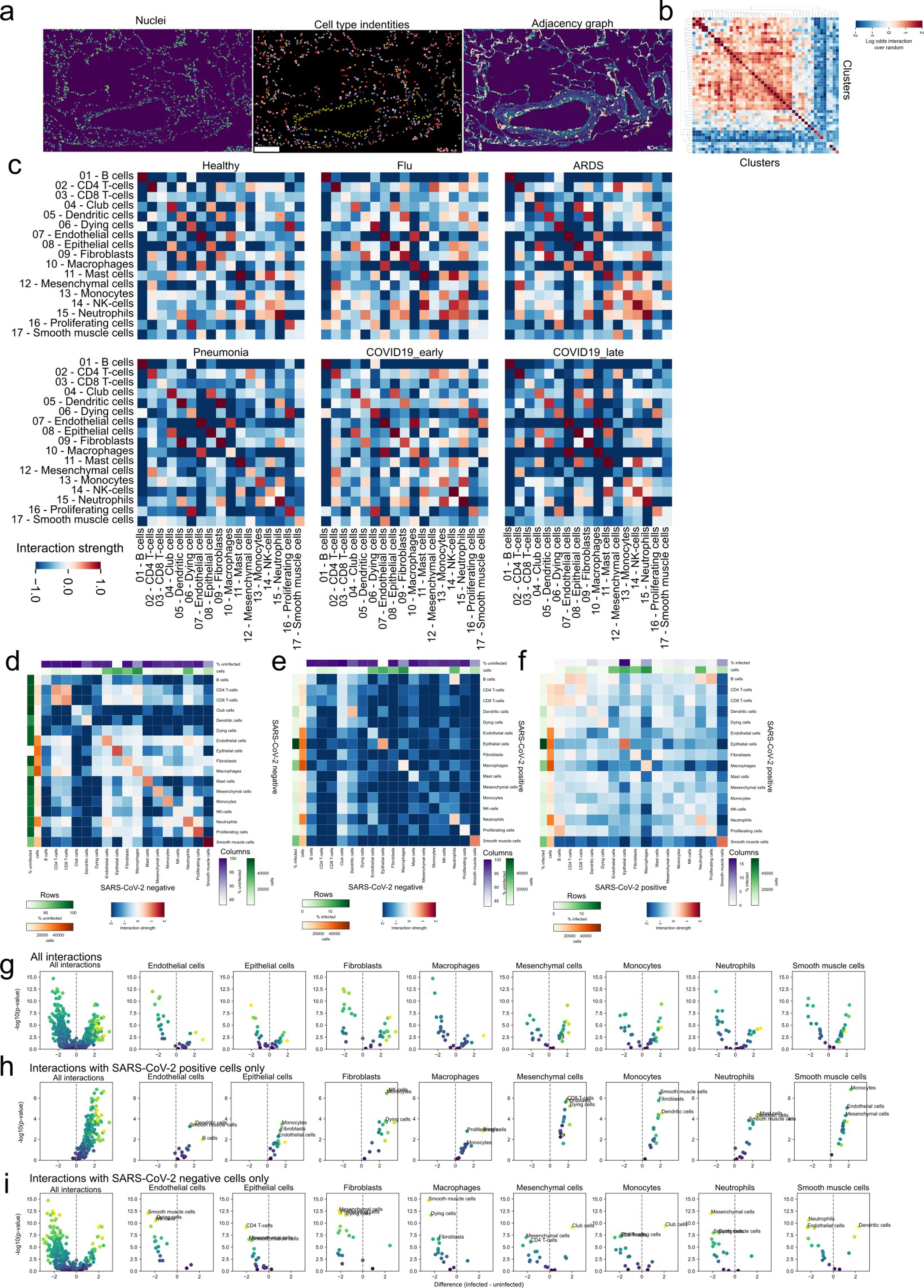
a) Exemplary description of the derivation of a Region Adjacency Graph (RAG) for a given lung IMC image. The leftmost image depicts the DNA channel marking nuclei, the centermost the identified meta-clusters, and the rightmost the RAG represented as edges between adjacent cells. Scale bar represents 100 microns. b) Observed values of pairwise cluster interactions over the expected values for the same cellular interactions for the image in a). c) Pairwise interactions between meta-clusters aggregated by the mean value across images depending on the disease group. d-f) Pairwise cellular interactions between meta-clusters dependent on SARS-CoV-2 Spike positivity: d) uninfected cells; e) between SARS-CoV-2 Spike positive and negative cells; f) between infected cells. g-i) Statistical testing of differential interactions of infected cells and other cell types and uninfected cells and other cell types, dependent on the SARS-CoV-2 Spike positivity of the second cell type: g) both SARS-CoV-2 Spike- and SARS-CoV-2 Spike+ cells; h) only SARS-CoV-2 Spike+ cells; i) only SARS-CoV-2 Spike- cells. The rows display a volcano plot where the x-axis display the difference in interaction between SARS-CoV-2 Spike+ and SARS-CoV-2 Spike- cells and the y-axis the -log10 Mann-Whitney U-test FDR-adjusted p-value.

Extended Data 9:

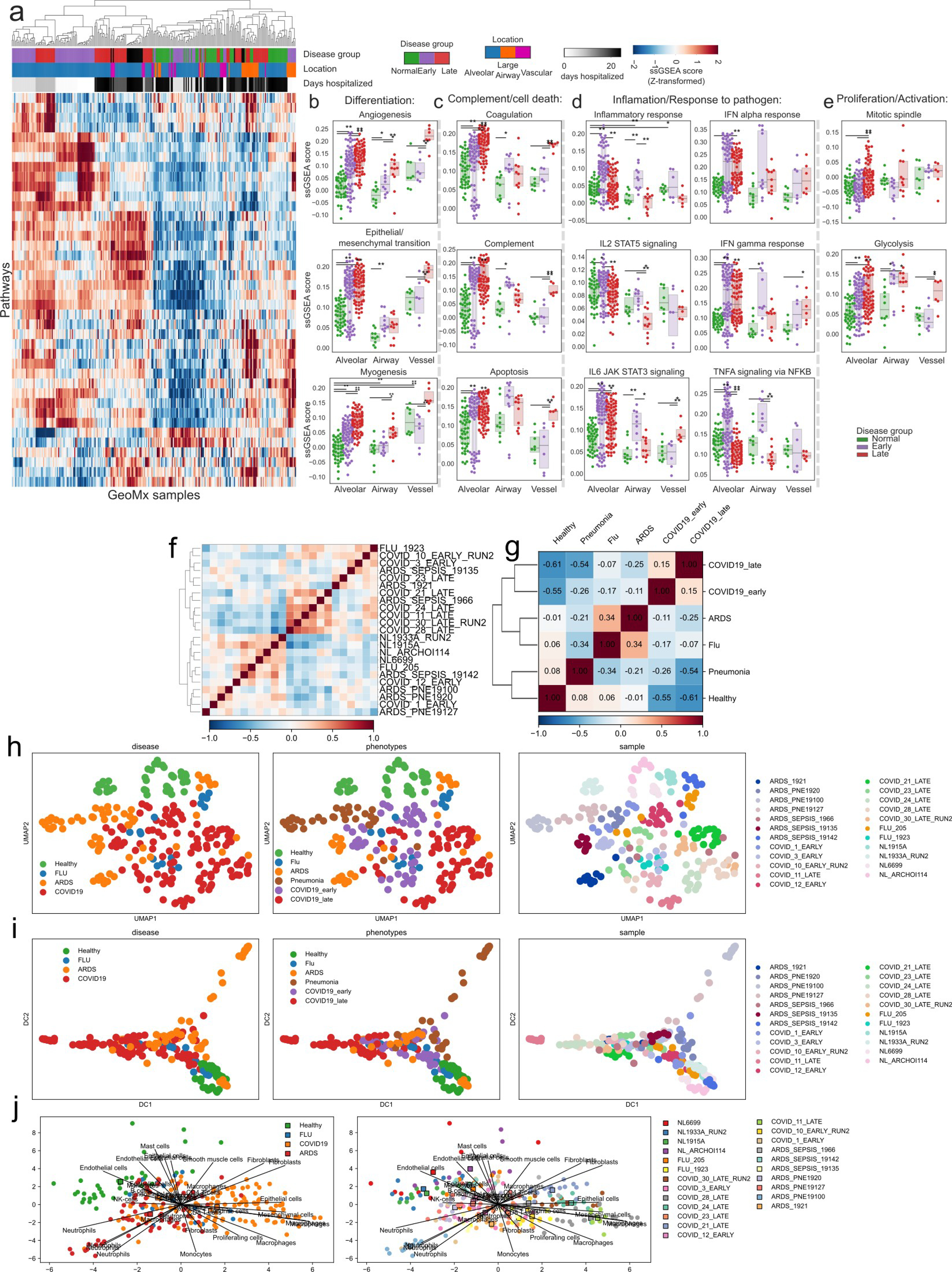
a) Enrichment scores for hallmark pathways in MsigDB across all ROIs in the GeoMx dataset. b-e) Enrichemnt score of selected pathways from a) across disease groups but dependent on the location within the lung from which they were obtained. ** p < 0.01; * p < 0.05, two-sided Mann-Whitney U-test, pairwise between groups, Benjamini-Hochberg FDR adjustment. f-g) Pairwise Pearson correlation of cell type abundances between f) IMC samples g) disease groups. h-j) h) UMAP, i) Diffusion map or j) PCA projection of IMC images colored by disease group, subgroup or sample ID.

Extended Data 10:

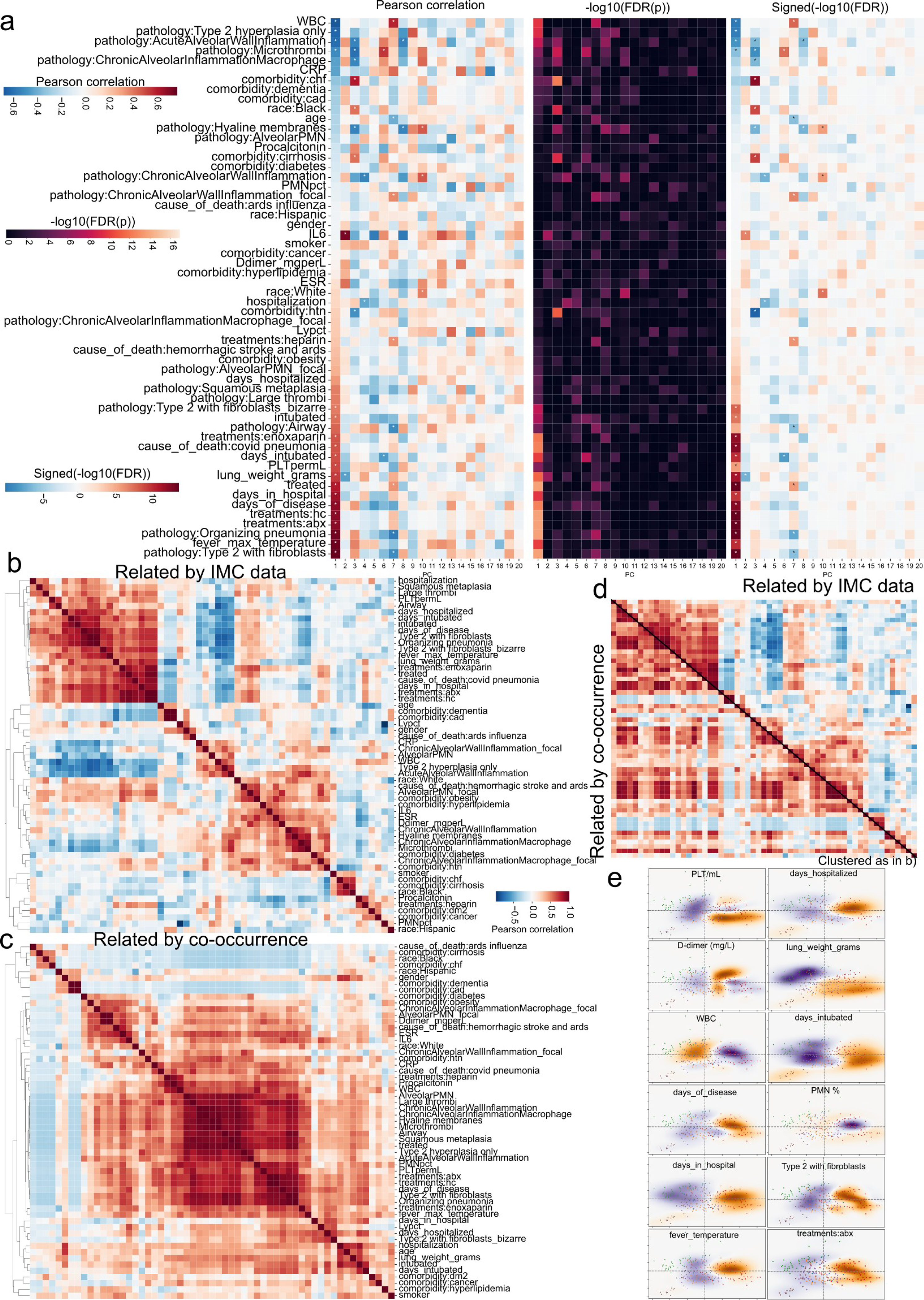
a) Correlation coefficients (left) or FDR-adjusted p-values (center) and signed p-values (right) demonstrating the association between demographic, pathologic, and clinical factors, and principal components. b) Pairwise correlation of demographic, pathologic, and clinical factors across all principal components. Matrix was clustered using average linking and pearson correlation as distance metric. Values used were signed FDR-adjusted p-values. c) Pairwise correlation of demographic, pathologic, and clinical factors across samples (co-occurrence). Matrix was clustered using average linking and pearson correlation as distance metric. d) Same as b) and c) where the top triangular matrix is from b) and the lower from c). The order of the rows and columns is the same as b). e) Projection of clinical factors onto pathology landscape. Kernel density estimation for various clinical and demographic factors weighted by the factor values, unweighted, or their difference.

Supplementary Material

Supplementary Table 2

List of metal-tagged antibodies used in imaging mass cytometry. Panel 1 (“Lung_COVID-19”) includes 36 markers characterizing immune cell phenotypes and functional markers related with COVID-19 such as IL-6, IL-1beta, cKIT, pSTAT3 and viral infection component S protein. Panel 2 (Immune activation) includes 38 markers characterizing immune cell activation states.

Supplementary Table 1

Detailed clinical annotations and demographic characteristics for patients included in the study representing different disease groups (ARDS post -viral influenza (n=2), ARDS post bacterial infection (n=4), bacterial pneumonia (n=3) and COVID-19 ARDS (n=10)) and control group (normal lung (n=4)).

Supplementary Table 3

Statistical testing of difference in abundance for clusters and meta-clusters between disease groups. A two tailed Mann-Whitney U-test was performed and p-values were adjusted with the Benjamini-Hochberg False Discovery Rate method. The uncorrected p-value is in the “p-unc” column, the corrected p-value in the “p-cor” column, and a measure of effect size is given in the “hedges” column, which indicates a Hedge’s g value.

Supplementary Table 4

Statistical testing of difference in fraction of cells positive in functional markers for clusters and meta-clusters between disease groups. A two tailed Mann-Whitney U-test was performed and p-values were adjusted with the Benjamini-Hochberg False Discovery Rate method. The uncorrected p-value is in the “p-unc” column, the corrected p-value in the “p-cor” column, and a measure of effect size is given in the “hedges” column, which indicates a Hedge’s g value.

References

- 1.Laing AG et al. A dynamic COVID-19 immune signature includes associations with poor prognosis. Nat. Med 26, 1623–1635 (2020). [DOI] [PubMed] [Google Scholar]
- 2.Lucas C et al. Longitudinal analyses reveal immunological misfiring in severe COVID-19. Nature 584, 463–469 (2020). [DOI] [PMC free article] [PubMed] [Google Scholar]
- 3.Mathew D et al. Deep immune profiling of COVID-19 patients reveals distinct immunotypes with therapeutic implications. Science 369, eabc8511 (2020). [DOI] [PMC free article] [PubMed] [Google Scholar]
- 4.Nienhold R et al. Two distinct immunopathological profiles in autopsy lungs of COVID-19. Nat. Commun 11, 5086 (2020). [DOI] [PMC free article] [PubMed] [Google Scholar]
- 5.Wang W et al. High-dimensional immune profiling by mass cytometry revealed immunosuppression and dysfunction of immunity in COVID-19 patients. Cell. Mol. Immunol 17, 650–652 (2020). [DOI] [PMC free article] [PubMed] [Google Scholar]
- 6.Unterman A et al. Single-cell omics reveals dyssynchrony of the innate and adaptive immune system in progressive COVID-19. Preprint at 10.1101/2020.07.16.20153437 (2020). [DOI] [PMC free article] [PubMed]
- 7.Takahashi T et al. Sex differences in immune responses that underlie COVID-19 disease outcomes. Nature 588, 315–320 (2020). [DOI] [PMC free article] [PubMed] [Google Scholar]
- 8.Hadjadj J et al. Impaired type I interferon activity and inflammatory responses in severe COVID-19 patients. Science 369, 718–724 (2020). [DOI] [PMC free article] [PubMed] [Google Scholar]
- 9.Giesen C et al. Highly multiplexed imaging of tumor tissues with subcellular resolution by mass cytometry. Nat. Methods 11, 417–422 (2014). [DOI] [PubMed] [Google Scholar]
- 10.McInnes L, Healy J, Saul N & Großberger L UMAP: uniform manifold approximation and projection. J. Open Source Softw 3, 861 (2018). [Google Scholar]
- 11.Dong E, Du H & Gardner L An interactive web-based dashboard to track COVID-19 in real time. Lancet Infect. Dis 20, 533–534 (2020). [DOI] [PMC free article] [PubMed] [Google Scholar]
- 12.Manson JJ et al. COVID-19-associated hyperinflammation and escalation of patient care: a retrospective longitudinal cohort study. Lancet Rheumatol 2, e594–e602 (2020). [DOI] [PMC free article] [PubMed] [Google Scholar]
- 13.Tay MZ, Poh CM, Rénia L, MacAry PA & Ng LFP The trinity of COVID-19: immunity, inflammation and intervention. Nat. Rev. Immunol 20, 363–374 (2020). [DOI] [PMC free article] [PubMed] [Google Scholar]
- 14.Grasselli G et al. Pathophysiology of COVID-19-associated acute respiratory distress syndrome: a multicentre prospective observational study. Lancet Respir. Med 8, 1201–1208 (2020). [DOI] [PMC free article] [PubMed] [Google Scholar]
- 15.Sinha P et al. Prevalence of phenotypes of acute respiratory distress syndrome in critically ill patients with COVID-19: a prospective observational study. Lancet Respir. Med 8, 1209–1218 (2020). [DOI] [PMC free article] [PubMed] [Google Scholar]
- 16.Arunachalam PS et al. Systems biological assessment of immunity to mild versus severe COVID-19 infection in humans. Science 369, 1210–1220 (2020). [DOI] [PMC free article] [PubMed] [Google Scholar]
- 17.Liao M et al. Single-cell landscape of bronchoalveolar immune cells in patients with COVID-19. Nat. Med 26, 842–844 (2020). [DOI] [PubMed] [Google Scholar]
- 18.Reyes L et al. A type I IFN, prothrombotic hyperinflammatory neutrophil signature is distinct for COVID-19 ARDS. Preprint at 10.1101/2020.09.15.20195305 (2020). [DOI] [PMC free article] [PubMed]
- 19.Bradley BT et al. Histopathology and ultrastructural findings of fatal COVID-19 infections in Washington State: a case series. Lancet 396, 320–332 (2020). [DOI] [PMC free article] [PubMed] [Google Scholar]
- 20.Bengsch B et al. Deep spatial profiling of COVID19 brains reveals neuroinflammation by compartmentalized local immune cell interactions and targets for intervention. Preprint at 10.21203/rs.3.rs-63687/v1 (2020). [DOI]
- 21.Tian S et al. Pathological study of the 2019 novel coronavirus disease (COVID-19) through postmortem core biopsies. Mod. Pathol 33, 1007–1014 (2020). [DOI] [PMC free article] [PubMed] [Google Scholar]
- 22.Duffield JS, Lupher M, Thannickal VJ & Wynn TA Host responses in tissue repair and fibrosis. Annu. Rev. Pathol 8, 241–276 (2013). [DOI] [PMC free article] [PubMed] [Google Scholar]
- 23.Ashcroft T, Simpson JM & Timbrell V Simple method of estimating severity of pulmonary fibrosis on a numerical scale. J. Clin. Pathol 41, 467–470 (1988). [DOI] [PMC free article] [PubMed] [Google Scholar]
- 24.Merritt CR et al. Multiplex digital spatial profiling of proteins and RNA in fixed tissue. Nat. Biotechnol 38, 586–599 (2020). [DOI] [PubMed] [Google Scholar]
- 25.Desai N et al. Temporal and spatial heterogeneity of host response to SARS-CoV-2 pulmonary infection. Nat. Commun 11, 6319 (2020). [DOI] [PMC free article] [PubMed] [Google Scholar]
- 26.Jackson HW et al. The single-cell pathology landscape of breast cancer. Nature 578, 615–620 (2020). [DOI] [PubMed] [Google Scholar]
- 27.Berg S et al. ilastik: interactive machine learning for (bio)image analysis. Nat. Methods 16, 1226–1232 (2019). [DOI] [PubMed] [Google Scholar]
- 28.McQuin C et al. CellProfiler 3.0: next-generation image processing for biology. PLoS Biol. 16, e2005970 (2018). [DOI] [PMC free article] [PubMed] [Google Scholar]
- 29.Immerkær J Fast noise variance estimation. Comput. Vis. Image Underst 64, 300–302 (1996). [Google Scholar]
- 30.Donoho DL & Johnstone IM Ideal spatial adaptation by wavelet shrinkage. Biometrika 81, 425–455 (1994). [Google Scholar]
- 31.Kit O & Lüdeke M Automated detection of slum area change in Hyderabad, India using multitemporal satellite imagery. ISPRS J. Photogramm. Remote Sens 83, 130–137 (2013). [Google Scholar]
- 32.Wolf FA, Angerer P & Theis FJ SCANPY: large-scale single-cell gene expression data analysis. Genome Biol. 19, 15 (2018). [DOI] [PMC free article] [PubMed] [Google Scholar]
- 33.Traag VA, Waltman L & van Eck NJ From Louvain to Leiden: guaranteeing well-connected communities. Sci. Rep 9, 5233 (2019). [DOI] [PMC free article] [PubMed] [Google Scholar]
- 34.Pedregosa F & Varoquaux G Scikit-learn: machine learning in Python. J. Mach. Learn. Res 12, 2825–2830 (2011). [Google Scholar]
- 35.Davies DL & Bouldin DW A cluster separation measure. IEEE Trans. Pattern Anal. Mach. Intell PAMI-1, 224–227 (1979). [PubMed] [Google Scholar]
- 36.van der Walt S et al. scikit-image: image processing in Python. PeerJ 2, e453 (2014). [DOI] [PMC free article] [PubMed] [Google Scholar]
- 37.Hagberg AA, Schult DA & Swart PJ Exploring network structure, dynamics, and function using NetworkX. In Proc. 7th Python in Science Conference (SciPy2008) (eds. Varoquaux G et al.) 11–15 (2008). [Google Scholar]
- 38.Schmidt U, Weigert M, Broaddus C & Myers G in Medical Image Computing and Computer Assisted Intervention – MICCAI 2018 (eds Frangi AF et al.) 265–273 (Springer, 2018). [Google Scholar]
- 39.Vallat R Pingouin: statistics in Python. J. Open Source Softw 3, 1026 (2018). [Google Scholar]
- 40.Harris CR et al. Array programming with NumPy. Nature 585, 357–362 (2020). [DOI] [PMC free article] [PubMed] [Google Scholar]
- 41.Virtanen P et al. SciPy 1.0: fundamental algorithms for scientific computing in Python. Nat. Methods 17, 261–272 (2020). [DOI] [PMC free article] [PubMed] [Google Scholar]
Associated Data
This section collects any data citations, data availability statements, or supplementary materials included in this article.
Supplementary Materials