A Full Nesterov-Todd Step Infeasible Interior-point Method for Symmetric Optimization in the Wider Neighborhood of the Central Path

Abstract

In this paper, an improved Interior-Point Method (IPM) for solving symmetric optimization problems is presented. Symmetric optimization (SO) problems are linear optimization problems over symmetric cones. In particular, the method can be efficiently applied to an important instance of SO, a Controlled Tabular Adjustment (CTA) problem which is a method used for Statistical Disclosure Limitation (SDL) of tabular data. The presented method is a full Nesterov-Todd step infeasible IPM for SO. The algorithm converges to ε-approximate solution from any starting point whether feasible or infeasible. Each iteration consists of the feasibility step and several centering steps, however, the iterates are obtained in the wider neighborhood of the central path in comparison to the similar algorithms of this type which is the main improvement of the method. However, the currently best known iteration bound known for infeasible short-step methods is still achieved.

1. Introduction

Interior-Point Methods (IPMs) are theoretically powerful and numerically efficient iterative methods that are based on Newton’s method. However, unlike Newton’s method, IPMs guarantee convergence to the ε-approximate solution of a problem in a polynomial number of iterations. It would be ambitious to claim such a result for any optimization problem, however, this is the case for quite a large class of optimization problems that include well known and important optimization problems such as linear optimization (LO), quadratic optimization (QO), semidefinite optimization (SDO), conic optimization problems and many others. There is extensive literature on IPMs, the following reference [21, 26] and the references therein may serve as a good start.

IPMs have shown to be a good alternative to the classic simplex method and they can solve efficiently LO problems of large size. Moreover, they can be applied to important optimization problems not previously accessible by simplex-type methods such as conic optimization problems. The development of IPM presented in this paper was motivated by the desire to provide a theoretical foundation for the efficient solution of the conic formulation of the Controlled Tabular Adjustment (CTA) problem [13].

The CTA is a method of Statistical Disclosure Limitation (SDL) that was first introduced in [2, 6]. SDL is an increasingly important area of research and practice for the statistical agencies that collect data from individuals or enterprises and then release it to the public, researchers, and policymakers for statistical analysis and research. Prior to such a release, the collected data have to undergo some SDL procedure in order to guarantee the privacy and confidentiality of data providers. The goals of such procedures are two-fold: minimize the risk of disclosure of confidential information about data providers and, at the same time, maximize the amount of released information, that is, maximize the utility of the data for the legitimate data users. These are conflicting goals and therefore SDL practice as a whole can be thought of as a search for the solution of complex and multifaceted optimization problem: maximize the utility of the released data subject to some upper bound on disclosure risk. The way how utility and risk are formulated depends on the scenario of data release and on the data format.

Data can be released in two basic formats: microdata - a collection of individual records, and tabular data - a table of cumulative data that is obtained from cross-tabulations of attributes from microdata. CTA is a perturbative method of protecting tabular data when a specified subset of its cells, called sensitive cells, must be modified to avoid re-identification of an individual respondent. The goal of CTA is to guarantee that the modified value of a sensitive cell is outside of the disclosure- an interval that is determined by the data protector (usually a statistical agency). The remaining cells are minimally adjusted to satisfy table equations which usually represent the requirement that the sum of elements in each row and column should be constant and remain unchanged. Hence, the goal of the CTA is to find the closest safe table to the original table with respect to the constraints outlined above. The closeness of the original and modified table is measured by the weighted distance between the tables with respect to a certain norm. Most commonly used norms are ℓ₁ and ℓ₂ norms. Thus, the problem can be formulated as a minimization problem with the objective function being a particular weighted distance function and constraints being table equations and lower and upper bounds on the cell values.

ℓ₂-CTA reduces to a QO problem while ℓ₁-CTA is a convex but nonsmooth problem that can be reformulated as LO problem, however, the number of variables and inequality constraints doubles. Alternatively, in [13] a novel second-order cone (SOC) reformulation of ℓ₁-CTA is proposed that does not increase the dimension of the problem as much. As it is shown in [13], conic reformulation of ℓ₁-CTA is a viable alternative to LO reformulation of the problem.

Our motivation was to design an IPM to solve conic ℓ₁-CTA that has good theoretical convergence properties and it is practical to implement which includes the fact that the method can start with any starting point, feasible or infeasible. However, the method is more general, that is, it is designed to solve a more general class of problems, a class of LO problems over symmetric cones of which conic ℓ₁-CTA is just one instance. Nevertheless, the general formulations of CTA and conic reformulation will be listed in the next section as examples of problems to which the proposed method can be applied. These problems are called symmetric optimization (SO) problems. The paper is entirely devoted to the design and analysis of the method, including convergence and complexity analysis because these results are important in their own right. Implementation, numerical testing, and application to conic ℓ₁-CTA and other conic problems will be the subject of a separate paper.

Symmetric cones (SC) is an important class of cones that has been known for quite some time, however, more in the field of algebraic geometry than in the field of optimization. They can be defined in different ways but the one that has shown to be useful in optimization is that symmetric cones are cones consisting of squares of elements of the related Euclidean Jordan Algebras (EJAs). The basic definitions and concepts related to EJAs and corresponding SC that are pertinent to the development of the method in the paper are listed in the next section. Additionally, the classical monograph of Faraut and Koràny [7] provides a wealth of information on Jordan algebras, SCs, and related topics.

Güler [12] was first to realize that symmetric cones, serve as a unifying framework to which the important types of cones used in optimization, such as non-negative orthant, second-order cone, and cone of positive semidefinite matrices belong. That opened a whole new field of research of designing and analyzing optimization algorithms for the SO problems which is still very active today. Faybusovich [8] was the first to generalize IPMs from LO to SO by using EJAs, and associated SC. Subsequently, different versions of IPMs for SO and related optimization problems on SC have been developed (see, e.g., [11, 16, 19, 22, 24]). For an overview of the relevant results, we refer to the monograph on this subject [1] and the references therein.

A full Newton-step infeasible IPM for LO was first analyzed by Roos [20]. The method was generalized by Gu et al. [11] to SO by using the full Nesterov-Todd (NT) direction as a search direction. The obtained iteration bound coincides with the one derived for LO, where n is replaced by r, the rank of EJAs, and matches currently best-known iteration bounds for infeasible IPMs for SO.

In this paper, we present an infeasible full NT-step IPM for SO that is a generalization of the feasible IPM discussed in [25]. In particular, Lemma 2.3 and Lemma 2.5 from [25] were used to obtained convergence of the method in the wider neighborhood of the central path while still maintaining the best iteration bound known for these types of methods.

The outline of the paper is as follows. In Section 2 we briefly recall some important definitions and results on EJAs and symmetric cones that are needed in the paper. In addition, we give a brief description and formulation of CTA problem. In Section 3, we briefly recall the framework of the full-NT step feasible IPM for SO with its improved convergence and complexity analysis. The full-NT step infeasible IPM for SO with its convergence and complexity analysis is presented in Section 4. Finally, some concluding remarks follow in Section 5.

2. Preliminaries

2.1. Euclidean Jordan Algebras and Symmetric Cones

In this section, we recall some important definitions and results on EJAs and associated symmetric cones that will be used in the rest of the paper.

A comprehensive treatment of EJAs and SCs can be found in the monograph [7] and in [1, 8, 9, 11, 22, 24] as it relates to optimization.

Definition 1

Let $(\mathcal{V},\langle \cdot ,\cdot \rangle )$ be an n-dimensional inner product space over R and ○ : (x, y) → x ○ y be a bilinear map from $\mathcal{V}\times \mathcal{V}$ to $\mathcal{V}$. Then $(\mathcal{V},○,\langle \cdot ,\cdot \rangle )$ (denoted by $\mathcal{V}$) is an EJA, if it satisfies the following conditions:

1. x ○ y = y ○ x for all $x,y\in \mathcal{V}$ (Commutativity)

2. x ○ (x²○ y) = x²○ (x ○ y) for all $x,y\in \mathcal{V}$, where x = x² ○ x (Jordan’s Axiom).

3. 〈x ○ y, z〉 = 〈x, y ○ z〉 for all $x,y,z\in \mathcal{V}$.

The operation, x ○ y is called the Jordan product of x and y. Moreover, we always assume that there exists an identity element $e\in \mathcal{V}$ such that e ○ x = x ○ e = x for all $x\in \mathcal{V}$.

For any element $x\in \mathcal{V}$, the Lyapunov transformation $L(x):\mathcal{V}\to \mathcal{V}$ is given by

$$L(x)y:=x○y,\forall y\in \mathcal{V}.$$ (1)

Furthermore, we define the quadratic representation of x in $\mathcal{V}$ as follows

$$P(x):=2L{(x)}^2-L\left(x^2\right),$$ (2)

where L(x)² = L(x)L(x).

In what follows we list some basic facts about symmetric cones.

Let V be a finite dimensional real Euclidean space. A nonempty subset $\mathcal{K}$ of V is a cone if $x\in \mathcal{K}$ and λ ≥ 0 a imply $\lambda x\in \mathcal{K}$. Cone $\mathcal{K}$ is a convex cone iff it is a cone and a convex set. The dual cone of a cone $\mathcal{K}$ is defined as a set ${\mathcal{K}}^{*}=\{y\in v:\forall x\in \mathcal{K},\langle x,y\rangle \ge 0\}$. It is straightforward to see that ${\mathcal{K}}^{*}$ is a closed convex cone. If $\mathcal{K}={\mathcal{K}}^{*}$, then $\mathcal{K}$ self-dual cone. Cone $\mathcal{K}$ is pointed cone if $\mathcal{K}\cap -\mathcal{K}=\left\{0\right\}$. In what follows we consider, convex, pointed cone $\mathcal{K}$. The interior of $\mathcal{K}$ is denoted as $\text{int}\mathcal{K}$.

A cone $\mathcal{K}$ is a SC if it is homogeneous and self-dual. A cone $\mathcal{K}$ is homogeneous if an automorphism group $Aut\left(\mathcal{K}\right)$ of $\mathcal{K}$ acts transitively on interior $\text{int}\mathcal{K}$ of a cone $\mathcal{K}$, that is, for all $x,y\in \text{int}\mathcal{K}$ there exists $g\in Aut(\mathcal{K})$ such that g(x) = y. Automorphism group is defined as $\mathit{\text{Aut}}(\mathcal{K})=\{g\in GL(V):g(\mathcal{K})=\mathcal{K}\}$ where GL(V) is a set of all invertible linear maps g : V → V

Let’s consider EJA $\mathcal{V}$, and a corresponding set of squares

$$\mathcal{K}(\mathcal{V}):=\left\{x^2:x\in \mathcal{V}\right\}$$ (3)

It can be shown that $\mathcal{K}\left(\mathcal{V}\right)$ is a SC (see, e.g., [7, 23]). This is the form of SC that will be used throughout the rest of the paper.

The importance of SC for optimization lays in the fact that common and frequently used cones used in optimization, such as non-negative orthant, SOC (ice cream cone), and semidefinite cone, the definitions of which are listed below, are all instances of SC.

1. The linear cone or non-negative orthant:

   $$\mathcal{K}={\text{R}}_{+}^{\text{n}}:=\left\{\text{x}\in {\text{R}}^{\mathrm{n}}:{\text{x}}_{\mathrm{i}}\ge 0,\text{i}=1,\dots ,\text{n}\right\}.$$
2. The positive semidefinite cone:

   $$\mathcal{K}=S_{+}^n:=\left\{X\in S^n:X⪰0\right\},$$

   where ⪰ means that X is positive semidefinite matrix and Sⁿ is a set of symmetric n-dimensional matrices.
3. The quadratic or SOC:

   $$\mathcal{K}={\mathcal{L}}^n=\left\{x\in {\text{R}}^{\mathrm{n}}:{\text{x}}_{\mathrm{i}}\ge \sqrt{{\text{x}}_1^2+\cdots +{\text{x}}_{\text{i}-1}^2+{\text{x}}_{\text{i}+1}^2+\cdots +{\text{x}}_{\mathrm{n}}^2}\right\}.$$

In what follows we define an important concept of a rank of EJA and describe two important decompositions of EJA, a spectral decomposition of an element in EJA and a Peirce decomposition of an EJA.

For any $x\in \mathcal{V}$, let r be the smallest integer such that the set {e, x, … , x^r} is linearly dependent. Then r is the degree of x which is denoted as deg(x). Clearly, this degree of x is bounded by the dimension of the vector space $\mathcal{V}$. Furthermore, there exist a polynomial p ≠ 0 such that p(x) = 0. If this polynomial has a leading coefficient one (monic polynomial) and the polynomial is of the minimal degree, then it is called minimal polynomial of element x. The rank of $\mathcal{V}$, denoted by $\text{rank}\left(\mathcal{V}\right)$, is the largest deg(x) of any element $x\in \mathcal{V}$. An element $x\in \mathcal{V}$ is called regular if its degree equals the rank of $\mathcal{V}$. In the sequel, $\mathcal{V}$ denotes an EJA with $\text{rank}\left(\mathcal{V}\right)=r$, unless stated otherwise.

For a regular element $x\in \mathcal{V}$, since {e, x, x², … , x^r} is linearly dependent, there are real numbers a₁(x), ⋯ , a_r(x) such that the minimal polynomial of x is given by

$$f(\lambda ;x)={\lambda }^r-a_1(x){\lambda }^{r-1}+\cdots +{(-1)}^r{a}_r(x).$$ (4)

Hence f(x; x) = 0. The polynomial f(λ; x) is called a characteristic polynomial of a regular element x. Hence, for regular elements, the minimal and characteristic polynomial coincide, however, for elements that are not regular, that may not be the case. Additionally, it can be proved that if regular element x vary, then a₁(x), ⋯ , a_r(x) are polynomials in x (Proposition II.2.1 in [7]). The coefficient a₁(x) is called the trace of x, denoted as tr(x). And the coefficient a_r(x) is called the determinant of x, denoted as det(x).

An element $c\in \mathcal{V}$ is said to be an idempotent if c² = c. Two idempotents c₁ and c₂ are said to be orthogonal if c₁ ○ c₂ = 0. Moreover, an idempotent is primitive if it is non-zero and cannot be written as the sum of two (necessarily orthogonal) non-zero idempotents. We say that {c₁, … , c_r} is a complete system of orthogonal primitive idempotents, or Jordan frame, if each c_i is a primitive idempotent, c_i ○ c_j = 0, i ≠ j, and ${\sum }_{i=1}^r{c}_i=e$. The Löwner partial ordering “${⪰}_{\mathcal{K}}$” of $\mathcal{V}$ defined by a cone $\mathcal{K}$ is defined by $x{⪰}_{\mathcal{K}}$ s if $x-s\in \mathcal{K}$. Likewise, $x{\succ }_{\mathcal{K}}$ s if $x-s\in \text{int}\mathcal{K}$.

The following theorem describes a spectral decomposition of elements of EJA $\mathcal{V}$, which plays an important role in the analysis of the IPMs for SO and other optimization problems.

Theorem 1

(Theorem III.1.2 in [7]) Let $x\in \mathcal{V}$. Then there exist a Jordan frame {c₁, … , c_r} and real numbers λ₁(x), … , λ_r(x) such that

$$x=\sum _{i=1}^r{\lambda }_i(x)c_i.$$ (5)

The numbers λ_i(x) (with their multiplicities) are the eigenvalues of x. Furthermore, the trace and the determinant of x are given by

$$\text{tr}(x)=\sum _{i=1}^r{\lambda }_i(x)\text{and det}(x)=\prod _{i=1}^r{\lambda }_i(x),$$ (6)

respectively.

For a fixed Jordan frame {c₁ ,c₂, … , c_r} in a EJA $\mathcal{V}$ and for i, j ∈ {1, 2, … , r}, we define the following eigenspaces

$${\mathcal{V}}_{ii}:=\left\{x\in \mathcal{V}:x○c_i=x\right\}=\text{R}{\text{c}}_{\mathrm{i}},{\mathcal{V}}_{\text{ij}}:=\left\{\text{x}\in \mathcal{V}:\text{x}○{\text{c}}_{\mathrm{i}}=\frac{1}{2}\text{x}=\text{x}○{\text{c}}_{\mathrm{j}}\right\},\text{i}\ne \text{j}.$$

The theorem below provides another important decomposition, the Peirce decomposition, of the space $\mathcal{V}$.

Theorem 2

(Theorem IV.2.1 in [7]) The space $\mathcal{V}$ is the orthogonal direct sum of the spaces ${\mathcal{V}}_{ij}(i\le j)$, i.e.,

$$\mathcal{V}=\underset{i\le j}{\oplus }{\mathcal{V}}_{ij}.$$

Furthermore,

$${\mathcal{V}}_{ij}○{\mathcal{V}}_{ij}\subset {\mathcal{V}}_{ii}+{\mathcal{V}}_{jj},{\mathcal{V}}_{ij}○{\mathcal{V}}_{jk}\subset {\mathcal{V}}_{ik},\text{if}i\ne k,{\mathcal{V}}_{ij}○{\mathcal{V}}_{kl}=\left\{0\right\},\text{if}\{i,j\}\cap \{k,l\}=\cancel{0}.$$

Thus, the Peirce decomposition of $x\in \mathcal{V}$ with respect to the Jordan frame {c₁, … , c_r} is given by

$$x=\sum _{i=1}^r{x}_i{c}_i+\sum _{i<j}{x}_{ij}$$ (7)

with x_i ∈ R, i = 1, … , r and $x_{ij}\in {\mathcal{V}}_{ij}$, 1 ≤ i < j ≤ r.

As a consequence of Theorem 2, we have the following corollary.

Corollary 1

(Lemma 12 in [22]) Let $x\in \mathcal{V}$ and its spectral decomposition with respect to the Jordan frame {c₁, … , c_r} is given by (5). Then the following statements hold.

1. The matrices, L(x) and P(x) commute and thus share a common system of eigenvectors; in fact the c_i, 1 ≤ i ≤ r are among their common eigenvectors.

2. The eigenvalues of L(x) have the form $\frac{{\lambda }_i+{\lambda }_j}{2}$, 1 ≤ i ≤ j ≤ r.

3. The eigenvalues of P(x) have the form λ_iλ_j, 1 ≤ i ≤ j ≤ r.

As already indicated, for any x, $s\in \mathcal{V}$, the trace inner product is given by

$$\langle x,s\rangle :=\text{tr}(x○s).$$ (8)

Thus, tr(x) = 〈x, e〉. Hence, it is easy to verify that

$$\text{tr}(x+s)=\text{tr}(x)+\text{tr}(s)\text{and}x{\underset{\_}{\prec }}_{\mathcal{K}}s\Rightarrow \text{tr}(x)\le \text{tr}(s).$$ (9)

The Frobenius norm induced by this trace inner product is then defined by

$$\Vert x{\Vert }_F:=\sqrt{\langle x,x\rangle }.$$ (10)

It follows from Theorem 1 that

$$\Vert x{\Vert }_F=\sqrt{\text{tr}\left(x^2\right)}=\sqrt{\sum _{i=1}^r{\lambda }_i^2(x)}.$$ (11)

One can easily verify that

$$\left|{\lambda }_{min}(x)\right|\le \Vert x{\Vert }_F\text{and}\left|{\lambda }_{max}(x)\right|\le \Vert x{\Vert }_F.$$ (12)

Furthermore, we have

$${\Vert x^2\Vert }_F\le {\Vert x\Vert }_F^2.$$ (13)

In the following lemmas, we recall several important inequalities used later in the paper.

Lemma 1

(Lemma 2.13 in [11]) Let x, $s\in \mathcal{V}$ and 〈x, s〉 = 0. Then

$$-\frac{1}{4}\Vert x+s{\Vert }_F^{2}e{\underset{\_}{\prec }}_{\mathcal{K}}x○s{\underset{\_}{\prec }}_{\mathcal{K}}\frac{1}{4}\Vert x+s{\Vert }_F^{2}e.$$

Lemma 2

(Lemma 2.16 in [11]) Let x, $s\in \mathcal{V}$. Then

$$\Vert x○s{\Vert }_F\le \frac{1}{2}{\Vert x^2+s^2\Vert }_F.$$

Next lemma provides an important inequality connecting eigenvalues of x ○ s with the sum of Frobenius norms of x and s.

Lemma 3

(Lemma 2.3 in [25]) Let x, $s\in \mathcal{V}$. Then

$$\sum _{i=1}^r\left|{\lambda }_i(x○s)\right|\le \frac{1}{2}\left(\Vert x{\Vert }_F^2+\Vert s{\Vert }_F^2\right).$$

If 〈x, s〉 = 0, then $\Vert x+s{\Vert }_F^2=\Vert x{\Vert }_F^2+\Vert s{\Vert }_F^2$. Thus, the following corollary follows immediately from Lemma 3.

Corollary 2

Let x, $s\in \mathcal{V}$ and 〈x, s〉 = 0. Then

$$\sum _{i=1}^r\left|{\lambda }_i(x○s)\right|\le \frac{1}{2}\Vert x+s{\Vert }_F^2.$$

Lemma 4

(Lemma 2.5 in [25]) Let u, $v\in \mathcal{V}$ and 〈u, v〉 = 0, and suppose ‖u + v‖_F = 2a with a < 1. Then

$$\langle e,{(e+u○v)}^{-1}-e\rangle \le \frac{2a^4}{1-a^4}.$$

Lemmas 3 and 4 are crucial in developing the improved complexity analysis of the algorithm presented in the next Section 3.

2.2. Continuous Tabular Adjustment Problem

In this subsection we provide the formulation of CTA problem as an important example of the conic problem to which the IPM developed in this paper can be efficiently applied.

The following CTA formulation is given in [13] and several other papers: Given the following set of parameters:

1. A set of cells a_i, $i\in \mathcal{N}=\{1,\dots ,n\}$. The vector a = (a₁, … , a_n)^T satisfies certain linear system Aa = b where A ∈ R^m×n is an m × n matrix and and b ∈ R^m is m-vector. The system usually decribes the fact that sum of elements in each row and column should remain unchanged, i.e. constant.

2. A lower, and upper bound for each cell, $l_{a_i}\le a_i\le u_{a_i}$ for $i\in \mathcal{N}$, which are considered known by any attacker.

3. A set of indices of sensitive cells, $\mathcal{S}=\left\{i_1,i_2,\dots ,i_s\right\}\subseteq \mathcal{N}$.

4. A lower and upper protection level for each sensitive cell $i\in \mathcal{S}$ respectively, lpl_i and upl_i, such that the released values must be outside of the interval (a_i − lpl_i, a_i + upl_i).

5. A set of weights, w_i, $i\in \mathcal{N}$ used in measuring the deviation of the released data values from the original data values.

A CTA problem is a problem of finding values z_i, $i\in \mathcal{N}$, such that z_i, $i\in \mathcal{S}$ are safe values and the weighted distance between released values z_i and original values a_i, denoted as ‖z – a‖_l(w), is minimized, which leads to solving the following optimization problem

$$\begin{array}{ll}\underset{z}{\text{min}}\hfill & \Vert z-a{\Vert }_{l(w)}\hfill \\ s.t.\hfill & Az=b,\hfill \\ \hfill & \begin{array}{l}{l}_{a_i}\le z_i\le u_{a_i},i\in \mathcal{N},\\ z_i,i\in \mathcal{S}\text{are}\text{safe}\text{values}.\end{array}\hfill \end{array}$$ (14)

As indicated in the assumption (iv) above, safe values are the values that satisfy

$$z_i\le a_i-lp{l}_i\text{or}{z}_i\ge a_i+up{l}_i,i\in \mathcal{S}.$$ (15)

By introducing a vector of binary variables y ∈ {0, 1}^s the constraint (15) can be written as

$$\begin{array}{l}{z}_i\ge -M\left(1-y_i\right)+\left(a_i+up{l}_i\right)y_i,i\in \mathcal{S},\\ z_i\le M{y}_i+\left(a_i-lp{l}_i\right)\left(1-y_i\right),i\in \mathcal{S},\end{array}$$ (16)

where M ≫ 0 is a large positive number. Constraints (16) enforce the upper safe value if y_i = 1 or the lower safe value if y_i = 0.

Replacing the last constraint in the CTA model (14) with (16) leads to a mixed integer convex optimization problem (MIOP) which is, in general, a difficult problem to solve; however, it provides solutions with high data utility [3]. The alternative approach is to fix binary variables up front, which leads to a CTA that is a continuous convex optimization problem because all binary variables are replaced with values 0 or 1. The continuous CTA is easier to solve; however, the obtained solution may have a lower data utility because the optimal solution of the continuous CTA is either feasible or infeasible solution of the corresponding MIOP depending on the values that were assigned to the binary variables. The strategies on how to avoid a wrong assignment of binary variables that may result in the MIOP being infeasible are discussed in [4, 5].

In what follows, we consider a continuous CTA where binary variables in MIOP are fixed with certain values of 0 or 1, and vector z is replaced by the vector of cell deviations x = z − a. Then, the CTA (14) reduces to the following convex optimization problem:

$$\begin{array}{ll}\underset{x}{\text{min}}\hfill & \Vert x{\Vert }_{l(w)}\hfill \\ s.t.\hfill & Ax=0,\hfill \\ \hfill & l\le x\le u,\hfill \end{array}$$ (17)

where upper and lover bounds for x_i, $i\in \mathcal{N}$ are defined as follows:

$$l_i=\{\begin{array}{ll}up{l}_i\hfill & \text{ if }i\in \mathcal{S}\text{ and }{y}_i=1\hfill \\ l_{a_i}-a_i\hfill & \text{ if }(i\in \mathcal{N}\backslash \mathcal{S})\text{ or }\left(i\in \mathcal{S}\text{ and }{y}_i=0\right)\hfill \end{array}$$ (18)

$$u_i=\{\begin{array}{ll}-lp{l}_i\hfill & \text{ if }i\in \mathcal{S}\text{ and }{y}_i=0\hfill \\ u_{a_i}-a_i\hfill & \text{ if }(i\in \mathcal{N}\backslash \mathcal{S})\text{ or }\left(i\in \mathcal{S}\text{ and }{y}_i=1\right).\hfill \end{array}$$ (19)

The two most commonly used norms in problem (17) are the ℓ₁ and ℓ₂ norms. For the ℓ₂-norm the problem, (17) reduces to the following ℓ₂-CTA model:

$$\begin{array}{ll}\underset{x}{\text{min}}\hfill & \sum _{i=1}^n{w}_i{x}_i^2\hfill \\ s\text{.}t\text{.}\hfill & Ax=0,\hfill \\ \hfill & l\le x\le u.\hfill \end{array}$$ (20)

The above problem is a standard QO problem that can be efficiently solved using IPM or other methods.

For the ℓ₁-norm the problem, (17) reduces to the following ℓ₁-CTA model:

$$\begin{array}{ll}\underset{x}{\text{min}}\hfill & \sum _{i=1}^n{w}_i\left|x_i\right|\hfill \\ s\text{.}t\text{.}\hfill & Ax=0,\hfill \\ \hfill & l\le x\le u.\hfill \end{array}$$ (21)

The above ℓ₁-CTA model (21) is a convex optimization problem; however, the objective function is not differentiable at x = 0. Since most of the algorithms, including IPMs, require differentiability of the objective function, problem (21) needs to be reformulated.

The standard reformulation is the transformation of a model (21) to the following LO model:

$$\begin{array}{ll}\hfill \underset{x^{-},x^{+}}{\text{min}}& \sum _{i=1}^n{w}_i\left(x_i^{+}+x_i^{-}\right)\hfill \\ \hfill s.t.& A\left(x_i^{+}-x_i^{-}\right)=0,\hfill \\ \hfill & \begin{array}{l}{l}^{+}\le x^{+}\le u^{+},\\ l^{-}\le x^{-}\le u^{-},\end{array}\hfill \end{array}$$ (22)

where

$$x^{+}=\{\begin{array}{ll}x\hfill & \text{ if }x\ge 0\hfill \\ 0\hfill & \text{ if }x<0,\hfill \end{array}{x}^{-}=\{\begin{array}{ll}0\hfill & \text{ if }x>0\hfill \\ -x\hfill & \text{ if }x\le 0,\hfill \end{array}$$ (23)

The drawback of the above LO reformulation is that number of variables and inequality constraints doubles. In [13] an alternative SOC reformulation of ℓ₁-CTA is proposed where the dimension of the problem does not increases as much. It is based on the fact that absolute value has an obvious SOC representation since the epigraph of the absolute value function is exactly SOC, that is,

$$t_i=\left|x_i\right|\to {\mathcal{K}}_i=\left\{\left(x_i,t_i\right)\in {\text{R}}^2:{\text{t}}_{\mathrm{i}}\ge \sqrt{{\text{x}}_{\mathrm{i}}^2}\right\}.$$

A SOC formulation of the l1-CTA (21) is given below

$$\begin{array}{ll}\underset{x}{\text{min}}\hfill & \sum _{i=1}^n{w}_i{t}_i\hfill \\ s.t.\hfill & Ax=0,\hfill \\ \hfill & \begin{array}{l}\left(x_i,t_i\right)\in {\mathcal{K}}_i;i=1,\dots ,n,\\ l\le x\le u.\end{array}\hfill \end{array}$$ (24)

The above conic formulation of continuous CTA problem is an important example of the conic problem to which the IPM developed and analyzed in the rest this paper can be efficiently applied.

3. A Brief Outline of the Full NT-Step Feasible IPM

In this section, a brief outline of the feasible algorithm presented in [25] is given.

Let $(\mathcal{V},○)$ be an n-dimensional EJA with rank r equipped with the standard inner product 〈x, s〉 = tr(x ○ s) and $\mathcal{K}$ be the corresponding symmetric cone. Moreover, we always assume that there exists an identity element $e\in \mathcal{V}$ such that e ○ x = x for all $x\in \mathcal{V}$. Additional facts regarding EJAs and SCs are listed in the previous Section 2 and references cited in that section.

We consider the LO problem over symmetric cones, or shortly, the SO problem given in the standard form

$$\begin{array}{lll}(SOP)\hfill & \text{min}\hfill & \langle c,x\rangle \hfill \\ \hfill & \text{s.t.}\hfill & Ax=b,x\in \mathcal{K},\hfill \end{array}$$

and its dual problem

$$\begin{array}{lll}\hfill (SOD)\hfill & \text{max}\hfill & b^{T}y\hfill \\ \hfill & \hfill \text{s.t.}\hfill & A^{T}y+s=c,s\in \mathcal{K},\hfill \end{array}$$

where A is a linear operator from $\mathcal{V}\text{to}{R}^m$, c and the rows of A lie in $\mathcal{V}$, b ∈ R^m, and A^T is the adjoint of A. Let $a_i\in \mathcal{V}$ be the ith row of A, then Ax = b means that 〈a_i, x〉 = b_i, for each i = 1, … , m, while A^Ty + s = c means that ${\sum }_{i=1}^m{y}_i{a}_i+s=c$. Without loss of generality, we assume that the rows of A are linearly independent.

Additionally, without loss of generality we can assume that both (SOP) and (SOD) satisfy the interior-point condition (IPC) [22], i.e., there exists (x⁰, y⁰, s⁰) such that

$$A{x}^0=b,x^0\in \text{int}\mathcal{K},A^T{y}^0+s^0=c,s^0\in \text{int}\mathcal{K}.$$

The perturbed Karush-Kuhn-Tucker (KKT) conditions for (SOP) and (SOD) are given by

$$\begin{array}{lll}\hfill Ax& =\hfill & b,x\in \mathcal{K},\hfill \\ \hfill A^{T}y+s& =\hfill & c,s\in \mathcal{K},\hfill \\ \hfill x○s& =\hfill & \mu e.\hfill \end{array}$$ (25)

The parameterized system (25) has a unique solution (x(μ), y(μ), s(μ)) for each μ > 0. The set of μ-centers forms a homotopy path with μ running through all positive real numbers, which is called the central path. If μ → 0, then the limit of the central path exists and since the limit points satisfy the complementarity condition, i.e., x ○ s = 0, it naturally yields an optimal solution for (SOP) and (SOD) (see, e.g., [8, 22]).

IPMs follow the central path approximately and find an approximate solution of the underlying problems (P) and (D) as μ gradually decreases to zero. Just like the case of a linear SDO, linearizing the third equation in (25) may not lead to an unique element in $\mathcal{V}$. Thus it is necessary to symmetrize that equation before linearizing it. To overcome this difficulty, the third equation of the system (25) is replaced by the following equivalent scaled equation (Lemma 28 in [22])

$$P(u)x○P\left(u^{-1}\right)s=\mu e,$$

where u is a scaling point from the interior of the cone $\mathcal{K}$ (i.e., $\text{int}\mathcal{K}$).

Applying Newton’s method, we have

$$\begin{array}{lll}\hfill A\Delta x& =\hfill & 0,\hfill \\ \hfill A^T\Delta y+\Delta s& =\hfill & 0,\hfill \\ \hfill P(u)x○P\left(u^{-1}\right)\Delta s+P\left(u^{-1}\right)s○P(u)\Delta x& =\hfill & \mu e-P(u)x○P\left(u^{-1}\right)s.\hfill \end{array}$$ (26)

The appropriate choices of u that lead to obtaining the unique search directions from the above system are called commutative class of search directions (see, e.g., [22]). In this paper, we consider the so-called NT-scaling scheme, the resulting direction is called NT search direction. This scaling scheme was first proposed by Nesterov and Todd [17, 18] for self-scaled cones and then adapted by Faybusovich [8, 9] for symmetric cones.

Lemma 5 (Lemma 3.2 in [9])

Let x, $s\in \text{int}\mathcal{K}$. Then there exists a unique $w\in \text{int}\mathcal{K}$ such that

$$x=P(w)s.$$

Moreover,

$$w=P{(x)}^{\frac{1}{2}}{\left(P\left(x^{\frac{1}{2}}\right)s\right)}^{-\frac{1}{2}}\left[=P\left(s^{-\frac{1}{2}}\right){\left(P\left(s^{\frac{1}{2}}\right)x\right)}^{\frac{1}{2}}\right].$$

The point w is called the scaling point of x and s (in this order). Let $u=w^{-\frac{1}{2}}$, where w is the NT-scaling point of x and s. Introducing the variance vector

$$v:=\frac{P{(w)}^{-\frac{1}{2}}x}{\sqrt{\mu }}\left[=\frac{P{(w)}^{\frac{1}{2}}s}{\sqrt{\mu }}\right],$$ (27)

and the scaled search directions

$$d_x:=\frac{P{(w)}^{-\frac{1}{2}}\Delta x}{\sqrt{\mu }}\text{and}{d}_s:=\frac{P{(w)}^{\frac{1}{2}}\Delta s}{\sqrt{\mu }},$$ (28)

the system (26) is further simplified

$$\begin{array}{lll}\hfill \overline{A}{d}_x& =\hfill & 0,\hfill \\ \hfill {\overline{A}}^T\Delta y+d_s& =\hfill & 0,\hfill \\ \hfill d_x+d_s& =\hfill & v^{-1}-v,\hfill \end{array}$$ (29)

where $\overline{A}:=\frac{1}{\sqrt{\mu }}AP{(w)}^{\frac{1}{2}}$. This system has a unique solution (d_x, Δy, d_s). The original search directions can then be obtained through (28). If (x, y, s) ≠ (x(μ), y(μ), s(μ)), then (Δx, Δy, Δs) is nonzero. The new iterate is obtained by taking full NT-steps

$$x^{+}:=x+\Delta x,y^{+}:=y+\Delta y,\text{and}{s}^{+}:=s+\Delta s.$$ (30)

From the first two equations of the system (29), one can easily verify that the scaled search directions d_x and d_s are orthogonal with respect to the trace inner product, i.e., 〈d_x, d_s〉=0. This implies that Δx and Δs also are orthogonal, i.e., 〈Δx, Δs〉=0. As a consequence, we have the important property that, after a full NT-step, the duality gap assumes the same value as at the μ-centers, namely rμ.

Lemma 6 (Lemma 3.4 in [11])

After a full NT-step, the duality gap is given by

$$\langle x^{+},s^{+}\rangle =r\mu .$$

To measure the distance of an iterate to the corresponding μ-center, a norm-based proximity measure δ(x, s; μ) is introduced

$$\delta (v):=\delta (x,s;\mu ):=\frac{1}{2}{\Vert v^{-1}-v\Vert }_F.$$ (31)

One can easily verify that

$$\delta (v)=0\iff v=e\iff d_x=d_s=0\iff x○s=\mu e,$$ (32)

which implies that the value of δ(v) can indeed be considered as a measure of the distance between the given iterate and the corresponding μ-center.

It is crucial for us to investigate the effect on the proximity measure δ(x, s; μ) of a full NT-step to the target point (x(μ), y(μ), s(μ)). For this purpose, Wang et al. [25] established a sharper quadratic convergence result than the one mentioned in [11]. Their derivation is based on the generalization of Theorem II.52 in [21] for LO. This leads to a wider quadratic convergence neighborhood of the central path for the algorithm than the one used in [11].

Theorem 3 (Theorem 3.2 in [25])

Let δ := δ(x, s; μ) < 1. Then, the full NT-step is strictly feasible and

$$\delta \left(x^{+},s^{+};\mu \right)\le \frac{{\delta }^2}{\sqrt{2\left(1-{\delta }^4\right)}}.$$

The following corollary shows the quadratic convergence of the full NT-step to the target μ-center (x(μ), y(μ), s(μ)) in the wider neighborhood determined by $1/\sqrt[4]{2}$ as opposed to $1/\sqrt{2}$ in [11].

Corollary 3

Let $\delta :=\delta (x,s;\mu )\le \frac{1}{\sqrt[4]{2}}$. Then the full NT-step is strictly feasible and

$$\delta \left(x^{+},s^{+};\mu \right)\le {\delta }^2.$$

The following theorem investigates the effect on the proximity measure when (x, y, s) is kept fixed and μ is updated to μ⁺ = (1 − θ)μ.

Theorem 4 (Theorem 3.3 in [25])

Let δ := δ(x, s; μ) < 1 and μ⁺ = (1 − θ)μ with 0 < θ < 1. Then

$$\delta {\left(x,s;{\mu }^{+}\right)}^2=(1-\theta ){\delta }^2+\frac{r{\theta }^2}{4(1-\theta )}.$$

As a consequence of Theorem 3 and Theorem 4, the following corollary readily follows.

Corollary 4

Let $\delta :=\delta (x,s;\mu )\le \frac{1}{\sqrt[4]{2}}$ and $\theta =\frac{1}{\sqrt{2r}}$ with r ≥ 2. Then

$$\delta \left(x^{+},s^{+};{\mu }^{+}\right)\le \frac{1}{\sqrt[4]{2}}.$$

The following theorem provides an upper bound for the total number of the iterations produced by the full-NT step feasible IPM.

Theorem 5 (Theorem 3.4 in [25])

Let $\tau =\frac{1}{\sqrt[4]{2}}$ and $\theta =\frac{1}{\sqrt{2r}}$ with r ≥ 2. Then the feasible algorithm requires

$$O\left(\sqrt{r}\text{log}\frac{\langle x^0,s^0\rangle }{\epsilon }\right)$$

iterations to obtain an iterate (x, y, s) satisfying 〈x, s〉 ≤ ε which is an ε-approximate optimal solution of (SOP) and (SOD).

Thus, the feasible algorithm is well defined, globally convergent, and achieves quadratic convergence of full NT-steps in the wider neighborhood while still maintaining the best known iteration bound known for these types of methods, namely

$$O\left(\sqrt{r}\text{log}\frac{r{\mu }_0}{\epsilon }\right).$$

4. Full NT-Step Infeasible IPM

It is well known fact that finding strictly feasible starting point may be difficult. Thus, an infeasible IPM that does not require feasible starting point may be a good alternative. First, a brief outline of the infeasible algorithm is presented. Next, we concentrate on the convergence and complexity analysis of the algorithm. The method is similar to IPM presented in [11], however, with wider neighborhood and larger steps which impacts the convergence and complexity analysis. Allowing larger steps at each iteration while still maintaining the best known iteration bound for these types of methods and having a quadratic local convergence of the proximity measure at each iteration are another advantages of the method presented in this paper.

4.1. An Outline of the Full NT-Step Infeasible IPM

In what follows, we assume that the SO problem has an optimal solution (x*, s*) with vanishing duality gap, i.e., 〈x*, s*〉 = 0. Furthermore, we choose arbitrarily $\left(x^0,s^0\right)\in \text{int}\mathcal{K}$ and μ⁰ > 0 such that

$$x^0=\zeta e,y^0=0,s^0=\zeta e,\text{and}{\mu }^0={\zeta }^2,$$ (33)

as the starting point of the algorithm, where ζ is a (positive) number such that

$$x^{*}+s^{*}{\underset{\_}{\prec }}_{\mathcal{K}}\zeta e.$$ (34)

The initial values of the primal and dual residual vectors are denoted as

$$r_p^0=b-A{x}^0\text{and}{r}_d^0=c-A^T{y}^0-s^0,$$ (35)

respectively. In general, we have $r_p^0\ne 0$ and $r_d^0\ne 0$, i.e., the initial iterate is not feasible for SO. However, a sequence of perturbed problems is constructed below in a such a way that the initial iterate is strictly feasible for the first perturbed problem in the sequence.

For any ν with 0 < ν ≤ 1, the perturbed problems of SO given in the standard form

$$\begin{array}{lll}(SO{P}_v)\hfill & \text{min}\hfill & \langle c-\nu r_d^0,x\rangle \hfill \\ \hfill & \text{s.t.}\hfill & b-Ax=\nu r_p^0,x\in \mathcal{K},\hfill \end{array}$$

and its dual problem

$$\begin{array}{lll}(SO{D}_v)\hfill & \text{min}\hfill & {\left(b-\nu r_p^0\right)}^{T}y\hfill \\ \hfill & \text{s.t.}\hfill & c-A^{T}y-s=\nu r_d^0,s\in \mathcal{K}.\hfill \end{array}$$

It is obvious that x = x⁰ is a strictly feasible solution of (SOP_ν), and (y, s) = (y⁰, s⁰) is a strictly feasible solution of (SOD_ν) when ν = 1, that is, (SOP_ν) and (SOD_ν) satisfy the IPC for ν = 1 which then straightforwardly leads to the following lemma.

Lemma 7 (Lemma 4.1 in [11])

Let (SOP) and (SOD) be feasible and 0 < ν ≤ 1. Then, the perturbed problems (SOP_ν) and (SOD_ν) satisfy the IPC.

Let (SOP) and (SOD) be feasible and 0 < ν ≤ 1. Then Lemma 7 implies that the perturbed problems (SOP_ν) and (SOD_ν) satisfy the IPC, and therefore the following system

$$\begin{array}{lll}\hfill b-Ax& =\hfill & \nu r_p^0,x\in \mathcal{K},\hfill \\ \hfill c-A^{T}y-s& =\hfill & \nu r_d^0,s\in \mathcal{K},\hfill \\ \hfill x○s& =\hfill & \mu e,\hfill \end{array}$$ (36)

has a unique solution (x(μ, ν), y(μ, ν), s(μ, ν)), for every μ > 0 that is called a μ-center of the perturbed problems (SOP_ν) and (SOD_ν). Hence, the central paths of (SOP_ν) and (SOD_ν) exist.

The main idea of the infeasible algorithm is to simultaneously improve feasibility by reducing ν and optimality by reducing μ while keeping the iterates in the certain neighborhood of the central paths of (SOP_ν) and (SOD_ν).

Thus, it make sense to link the parameters μ and ν according to the following formula μ = νμ⁰ = νζ². It is also worth noting that, according to (33) , x⁰ ○ s⁰ = μ⁰e; hence, x⁰ is the μ⁰-center of the perturbed problem (SOP_ν), and (y⁰, s⁰) is the μ⁰-center of the perturbed problem (SOD_ν) for ν = 1. In other words,

$$\left(x\left({\mu }^0,1\right),y\left({\mu }^0,1\right),s\left({\mu }^0,1\right)\right)=\left(x^0,y^0,s^0\right)$$

and the algorithm can easily be started since we have initial starting point that is by construction exactly on the central path of (SOP_ν) and (SOD_ν) for ν = 1.

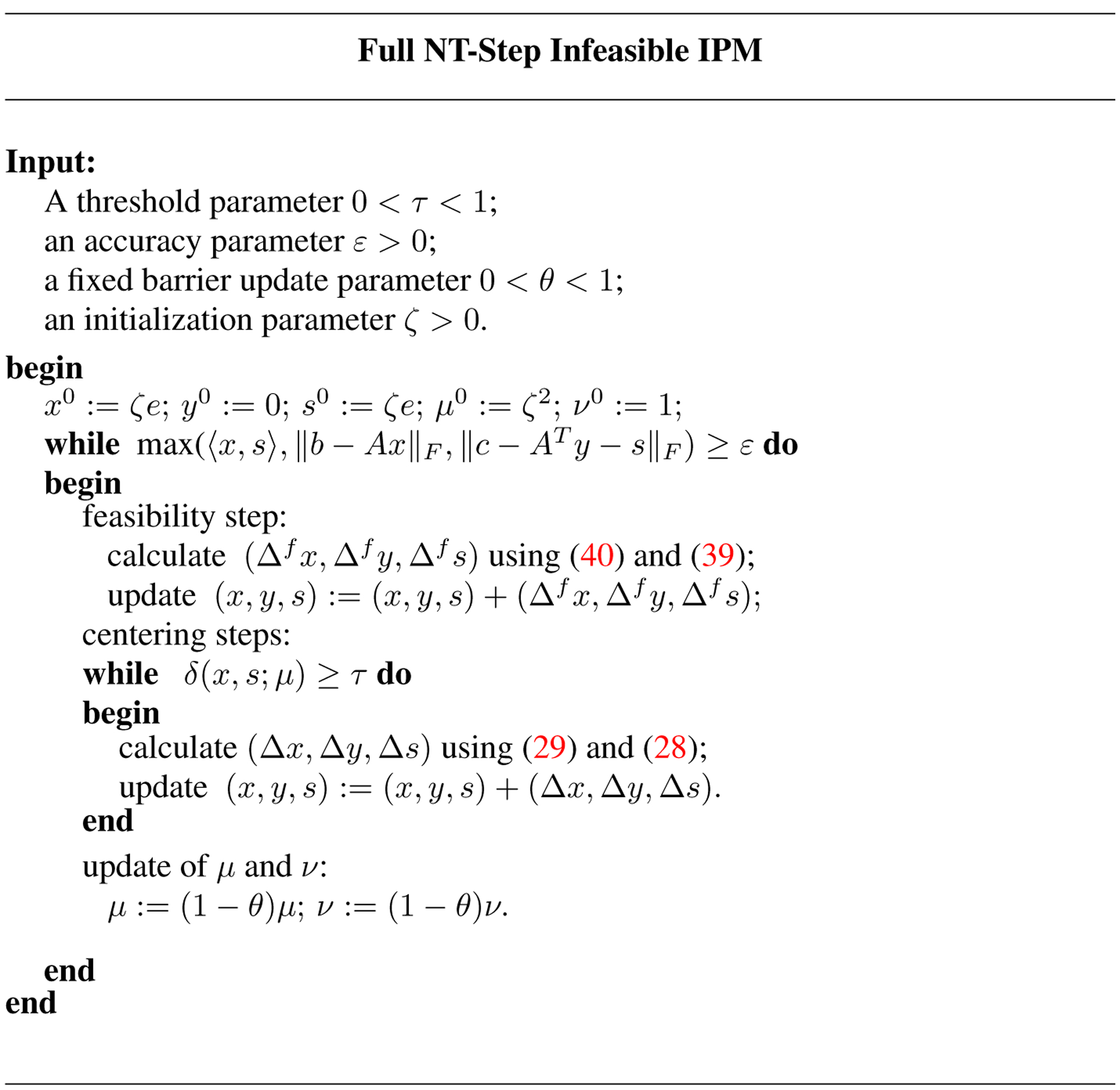
The outline of one iteration of the infeasible algorithm is as follows. Suppose that for some ν ∈ (0, 1] we have an iterate (x, y, s) satisfying the feasibility condition, i.e., the first two equations of the system (36) for μ = νμ⁰, and such that tr(x ○ s) = rμ and δ(x, s; μ) ≤ τ. Thus, we start with the iterate in the τ-neighborhood of the central path of (SOP_ν) and (SOD_ν) that targets the μ-center on that central path . The goal is to obtain a new iterate (x⁺, y⁺, s⁺) in the τ-neighborhood of the central path of the new pair of problems $\left(SO{P}_v^{+}\right)$ and $\left(SO{D}_v^{+}\right)$ where both ν and μ are reduced by a barrier parameter θ ∈ (0, 1), i.e., ν⁺ = (1 − θ)ν and μ⁺ = (1 − θ)μ = ν⁺μ⁰. Hence, (x⁺, y⁺, s⁺) should satisfy the first two equations of the system (36), with ν replaced by ν⁺ and μ by μ⁺, and such that tr(x⁺, s⁺) = rμ⁺ and δ(x⁺, s⁺; μ⁺) ≤ τ.

The calculation of the new iterate is achieved in two phases, a feasibility phase where one feasibility step is taken and a centering phase where a few centering steps are performed. The feasibility step serves to get an iterate (x^f, y^f, s^f) that is strictly feasible for $\left(SO{P}_{v^{+}}\right)$ and $\left(SO{D}_{v^{+}}\right)$, and belongs to the quadratic convergence neighborhood with respect to the μ⁺-center of $\left(SO{P}_{v^{+}}\right)$ and $\left(SO{D}_{v^{+}}\right)$. However, (x^f, y^f, s^f) may not be in the τ-neighborhood of the μ⁺-center; therefore, several centering steps may need to be performed to get inside the τ-neighborhood.

Note that after each iteration the residuals and the duality gap are reduced by the factor (1 − θ). The algorithm stops when we obtain an iterate for which the norm of the residuals and the duality gap do not exceed the accuracy parameter ε. This iterate is called an ε-approximate optimal solution for (SOP) and (SOD).

The feasibility step is obtained by taking full steps

$$x^f:=x+{\Delta }^{f}x,y^f:=y+{\Delta }^{f}y,\text{and}{s}^f:=s+{\Delta }^{f}s,$$ (37)

with NT-search directions (Δ^fx, Δ^fy, Δ^fs) that are calculated from the following Newton system

$$\begin{array}{lll}\hfill A{\Delta }^{f}x& =\hfill & \theta \nu r_p^0,\hfill \\ \hfill A^T{\Delta }^{f}y+{\Delta }^{f}s& =\hfill & \theta \nu r_d^0,\hfill \\ \hfill P{(w)}^{-\frac{1}{2}}x○P{(w)}^{\frac{1}{2}}{\Delta }^{f}s+P{(w)}^{\frac{1}{2}}s○P{(w)}^{-\frac{1}{2}}{\Delta }^{f}x& =\hfill & (1-\theta )\mu e-P{(w)}^{-\frac{1}{2}}x○P{(w)}^{\frac{1}{2}}s.\hfill \end{array}$$ (38)

One may easily verify that (x^f, y^f, s^f) satisfies the first two equations of the system (36), with ν replaced by ν⁺ and μ by μ⁺. The third equation indicates that the μ⁺-center of $\left(SO{P}_v^{+}\right)$ and $\left(SO{D}_v^{+}\right)$ is targeted. Targeting μ⁺center rather than μ-center contributes to the efficiency of the algorithm. The system (38) defines the feasibility step uniquely since the coefficient matrix of the resulting system is exactly the same as in the feasible case.

Similarly to the feasible case, given the variance vector v defined by (27) and scaled search directions

$$d_x^f:=\frac{P{(w)}^{-\frac{1}{2}}{\Delta }^{f}x}{\sqrt{\mu }}\text{and}{d}_s^f:=\frac{P{(w)}^{\frac{1}{2}}{\Delta }^{f}s}{\sqrt{\mu }},$$ (39)

the system (38) is reduced to the following form

$$\begin{array}{lll}\hfill \overline{A}{d}_x^f& =\hfill & \frac{1}{\mu }\theta \nu r_p^0,\hfill \\ \hfill {\overline{A}}^T{\Delta }^{f}y+d_s^f& =\hfill & \frac{1}{\sqrt{\mu }}\theta \nu P{(w)}^{\frac{1}{2}}{r}_d^0,\hfill \\ \hfill d_x^f+d_s^f& =\hfill & (1-\theta )v^{-1}-v.\hfill \end{array}$$ (40)

Hence,

$$x^f=x+{\Delta }^{f}x=\sqrt{\mu }P{(w)}^{\frac{1}{2}}\left(v+d_x^f\right)\text{and}{s}^f=s+{\Delta }^{f}s=\sqrt{\mu }P{(w)}^{-\frac{1}{2}}\left(v+d_s^f\right).$$ (41)

Since it will be shown that (x^f, y^f, s^f) is strictly feasible and moreover in the quadratic convergence neighborhood of the μ⁺-center of $\left(SO{P}_{v^{+}}\right)$ and $\left(SO{D}_{v^{+}}\right)$, it is possible to take few centering steps to get the new iteration in the desired τ-neighborhood of the μ⁺-center. The centering steps are obtained by taking full steps with NT-search directions calculated from the Newton system that is the same as in the feasible case, (26), or in the scaled form, (29).

The above outline is summarized in the Fig. 1, that describes a generic full NT-step infeasible IPM.

Figure 1.

Algorithm I

4.2. Analysis of the Full-NT Step Infeasible IPM

The analysis of the infeasible algorithm is more complicated and more involved than in the feasible case. The main reason for this is that the scaled search directions $d_x^f$ and $d_s^f$ are not (necessarily) orthogonal with respect to the trace inner product. We omit most parts of the analysis that are unchanged from the one presented in [11] and emphasize the parts where there are differences. It is shown that the feasibility steps can be taken in the wider quadratic convergence neighborhood of the central path developed in the feasible case.

Feasibility Step.

The lemma below provides the sufficient condition for the strict feasibility of the feasibility step (x^f, y^f, s^f).

Lemma 8 (Lemma 4.2 in [11])

The feasibility step (x^f, y^f, s^f) is strictly feasible if $(1-\theta )e+d_x^f○d_s^f\in \text{int}\mathcal{K}$.

Thus, the feasibility of the (x^f, y^f, s^f) highly depends on the eigenvalues of the vector $d_x^f○d_s^f$. More specifically, (x^f, y^f, s^f) is strictly feasible if ${\Vert \lambda \left(d_x^f○d_s^f\right)\Vert }_{\infty }<1-\theta$.

In order to measure the distance from the (x^f, y^f, s^f) to the. μ⁺-center we need an upper bound on the proximity measure δ(x^f,s^f;μ⁺) which is for simplicity denoted also as δ(v^f), where v^f is a variance vector defined by (27).

The following lemma provides an upper bound for δ(v^f).

Lemma 9 (Lemma 4.4 in [11])

Let ${\Vert \lambda \left(d_x^f○d_s^f\right)\Vert }_{\infty }<1-\theta$. Then

$$4\delta {\left(v^f\right)}^2\le \frac{{\Vert \frac{d_x^f○d_s^f}{1-\theta }\Vert }_F^2}{1-{\Vert \frac{\lambda \left(d_x^f○d_s^f\right)}{1-\theta }\Vert }_{\infty }}.$$

The following lemma gives an important relationship between the infinite norm of the vector of eigenvalues of d_x ○ d_s and the Frobenius norms of d_x and d_s.

Lemma 10

One has

$${\Vert \lambda \left(d_x^f○d_s^f\right)\Vert }_{\infty }\le {\Vert d_x^f○d_s^f\Vert }_F\le \frac{1}{2}\left({\Vert d_x^f\Vert }_F^2+{\Vert d_s^f\Vert }_F^2\right).$$

Proof

We have the following derivation:

$$\begin{array}{l}{\Vert \lambda \left(d_x^f○d_s^f\right)\Vert }_{\infty }\le {\Vert d_x^f○d_s^f\Vert }_F\le \frac{1}{2}{\Vert {\left(d_x^f\right)}^2+{\left(d_s^f\right)}^2\Vert }_F\\ \le \frac{1}{2}{\Vert {\left(d_x^f\right)}^2\Vert }_F+\frac{1}{2}{\Vert {\left(d_s^f\right)}^2\Vert }_F\le \frac{1}{2}\left({\Vert d_x^f\Vert }_F^2+{\Vert d_s^f\Vert }_F^2\right).\end{array}$$

The first inequality follows from the definitions of the infinite norm for vectors and the Frobenius norm for the element of $\mathcal{V}$. The second inequality follows from Lemma 2.16 in [11], the third inequality follows from the triangle inequality for the Frobenius norm, and the last inequality follows from Lemma 2.12 in [11]. This completes the proof of the lemma. □

Substitution of the two inequalities in Lemma 10 into the inequality in Lemma 9 yields the following upper bound

$$4\delta {\left(v^f\right)}^2\le \frac{{\Vert \frac{d_x^f○d_s^f}{1-\theta }\Vert }_F^2}{1-{\Vert \frac{\lambda \left(d_x^f○d_s^f\right)}{1-\theta }\Vert }_{\infty }}\le \frac{\frac{1}{4}{\left(\frac{{\Vert d_x^f\Vert }_F^2+{\Vert d_s^f\Vert }_F^2}{1-\theta }\right)}^2}{1-\frac{1}{2}\frac{{\Vert d_x^f\Vert }_F^2+{\Vert d_s^f\Vert }_F^2}{1-\theta }}.$$ (42)

Thus, a task of finding an upper bound of δ(v^f) reduces to finding an upper bound of ${\Vert d_x^f\Vert }_F^2+{\Vert d_s^f\Vert }_F^2$.

After careful and somewhat involved analysis, details of which are omitted and can be found in [11], the following upper bound is derived:

$${\Vert d_x^f\Vert }_F^2+{\Vert d_s^f\Vert }_F^2\le 2\left(4{(1-\theta )}^2{\delta }^2+{\theta }^{2}r\right)+12{\theta }^2{r}^2\rho {(\delta )}^2,$$ (43)

where δ := δ(v) and $\rho (\delta ):=\delta +\sqrt{1+{\delta }^2}$. Thus, the upper bound essentially depends on the barrier parameter θ and the proximity measure δ of the old iterate (x, y, s), which is a desired result since we want to connect new proximity measure with the old one.

In what follows, we want to choose θ, 0 < θ < 1, as large as possible, and such that (x^f, y^f, s^f) lies in the quadratic convergence neighborhood with respect to the μ⁺-center of the perturbed problems $\left(SO{P}_{v^{+}}\right)$ and $\left(SO{D}_{v^{+}}\right)$. As it was shown in the feasible case, this neighborhood can be extended to $\delta \left(v^f\right)\le 1/\sqrt[4]{2}$ as opposed to $\delta \left(v^f\right)\le 1/\sqrt{2}$ in [11].

From (42), we know that $\delta \left(v^f\right)\le 1/\sqrt[4]{2}$ holds if

$$\frac{\frac{1}{4}{\left(\frac{{\Vert d_x^f\Vert }_F^2+{\Vert d_s^f\Vert }_F^2}{1-\theta }\right)}^2}{1-\frac{1}{2}\frac{{\Vert d_x^f\Vert }_F^2+{\Vert d_s^f\Vert }_F^2}{1-\theta }}\le 2\sqrt{2},$$ (44)

which leads to the following inequality

$$\frac{{\Vert d_x^f\Vert }_F^2+{\Vert d_s^f\Vert }_F^2}{1-\theta }\le 2\sqrt{2}(\sqrt{1+\sqrt{2}}-1)\approx \mathrm{1.566.}$$ (45)

Substituting (43) into the above inequality (45) we obtain

$$2\left(4{(1-\theta )}^2{\delta }^2+{\theta }^{2}r\right)+12{\theta }^2{r}^2\rho {(\delta )}^2\le 2\sqrt{2}(\sqrt{1+\sqrt{2}}-1)(1-\theta ).$$ (46)

One can easily verify that the largest values of θ and τ for which inequality (45) holds are

$$\tau =\frac{1}{16}\text{and}\theta =\frac{1}{4r}.$$ (47)

Furthermore, from Lemma 10 and (45) we obtain

$$\Vert \lambda (d_x^f○d_s^f{\Vert }_{\infty }\le \frac{1}{2}\left({\Vert d_x^f\Vert }_F^2+{\Vert d_s^f\Vert }_F^2\right)\le \sqrt{2}(\sqrt{1+\sqrt{2}}-1)(1-\theta )<1-\theta .$$ (48)

Lemma 8 then implies that with the above choice of parameters θ and τ, (x^f, y^f, s^f) is indeed strictly feasible.

Centering Steps.

After the feasibility step we perform centering steps in order to get an iterate (x⁺, y⁺, s⁺) that is in the τ-neighborhood of the μ⁺-center, i.e. satisfies tr(x⁺ ○ s⁺) = rμ⁺ and δ(x⁺, s⁺; μ⁺) ≤ τ. Using Corollary 3, the required number of centering steps can easily be obtained. Indeed, since (x^f, y^f, s^f) is in the quadratic convergence neighborhood of the μ⁺-center, i.e. $\delta =\delta \left(x^f,s^f;{\mu }^{+}\right)\le 1/\sqrt[4]{2}$, after k centering steps we will have an iterate (x⁺, y⁺, s⁺) that is still feasible for $\left(SO{P}_{v^{+}}\right)$ and $\left(SO{D}_{v^{+}}\right)$ and satisfies

$$\delta \left(x^{+},s^{+};{\mu }^{+}\right)\le {\left(\frac{1}{\sqrt[4]{2}}\right)}^{2^k}.$$

Hence, δ(x⁺, y⁺, s⁺) ≤ τ is satisfied if k satisfies

$${\left(\frac{1}{\sqrt[4]{2}}\right)}^{2^k}\le \tau .$$

Thus, δ(x⁺, s⁺; μ⁺) ≤ τ will be obtained after at most

$$2+\lceil {\text{log}}_2\left({\text{log}}_2\frac{1}{\tau }\right)\rceil$$ (49)

centering steps.

Substituting τ = 1/16 into the above expression leads to

$$2+\lceil {\text{log}}_2\left({\text{log}}_2\left(\frac{1}{\tau }\right)\right)\rceil =2+\lceil {\text{log}}_2\left({\text{log}}_{2}16\right)\rceil =4.$$

Hence, at most four centering steps are needed to get the iterate (x⁺, y⁺, s⁺) that satisfies δ(x⁺, s⁺; μ⁺) ≤ τ, i.e., the iterate that is in the τ-neighborhood of the μ⁺-center again.

Iteration Bound.

To summarize, each main iteration consists of at most five inner iterations, one feasibility step, and at most four centering steps. In each main iteration both the duality gap and the norms of the residual vectors are reduced by the factor (1 − θ). Hence, using tr(x⁰ ○ s⁰) = rζ², the total number of main iterations is bounded above by

$$\frac{1}{\theta }\text{log}\frac{\text{max}\left\{r{\zeta }^2,{\Vert r_p^0\Vert }_F,{\Vert r_d^0\Vert }_F\right\}}{\epsilon }$$

Since $\theta =\frac{1}{4r}$ and at most five inner iterations per the main iteration are needed, the main result can be stated in the following theorem.

Theorem 6

Suppose (SOP) has an optimal solution x* and (SOD) has an optimal solution (y*, s*), which satisfy tr(x* ○ s*) = 0 and $x^{*}+s^{*}{\underset{\_}{\prec }}_{\mathcal{K}}\zeta e$ for some ζ > 0. If the values of parameters τ and θ are chosen as $\tau =\frac{1}{16}$ and $\theta =\frac{1}{4r}$, then at most

$$20r\text{log}\frac{\text{max}\left\{r{\zeta }^2,{\Vert r_p^0\Vert }_F,{\Vert r_d^0\Vert }_F\right\}}{\epsilon }$$

inner iterations of the algorithm in Fig. 1, are needed to find an ε-approximate optimal solution of (SOP) and (SOD).

In conclusion, the infeasible algorithm in Fig 1 is well defined, globally convergent, and achieves quadratic convergence of full NT-feasibility steps in the wider neighborhood of the central path while still maintaining the best-known iteration bound known for these types of methods, namely

$$O\left(r\text{log}\frac{\text{max}\left\{r{\zeta }^2,{\Vert r_p^0\Vert }_F,{\Vert r_d^0\Vert }_F\right\}}{\epsilon }\right).$$

Remark 1

Similarly to LO, the iteration bound in Theorem 6 is derived under the assumption that there exists an optimal solution pair (x*, y*, s*) of (SOP) and (SOD) with vanishing duality gap and satisfying $x^{*}+s^{*}{\underset{\_}{\prec }}_{\mathcal{K}}\zeta e$. During the course of the algorithm, if at some main iteration, the proximity measure δ after the feasibility step exceeds $1/\sqrt[4]{2}$, then it tells us that the above assumption does not hold. It may happen that the value of ζ has been chosen too small. In this case, one might run the algorithm once more with a larger value of ζ. If this does not help, then eventually one should realize that (SOP) and/or (SOD) do not have optimal solutions at all, or they have optimal solutions with a positive duality gap.

Remark 2

In [11] the number of centering steps per the main iteration is three. In our paper, the ‘price to pay for expanding the quadratic convergence neighborhood of the central path is a possible additional centering step which slightly increases the constant in the upper bound on the total number of inner iterations from 16 to 20; however, that does not change the order of magnitude of the required number of iterations, it still matches the best-known iteration bound for the infeasible algorithms mentioned above. It is also worth mentioning that in practice all four centering steps may not always be needed, very often only one or two suffice.

5. Concluding remarks

In this paper, an infeasible version of the full NT-step IPM for SO in a wider neighborhood of the central path than the one in [11] is presented and convergence analysis is given. Wider quadratic convergence neighborhood of the central path characterized by $1/\sqrt[4]{2}$ is carried over from the feasible case and applied to the feasibility steps of the infeasible algorithm resulting in larger steps. However, despite full NT-steps in the wider neighborhood of the central path, the best complexity known for the infeasible algorithm is still maintained.

Future research is planned in two directions. The first direction is implementation and numerical testing of the method on a set of conic CTA problems as well as other conic problems. The second direction is theoretical and involves the generalization of this IPM to other optimization problems such as Linear Complementarity Problems over symmetric cones.

REFERENCES

- [1].Anjos MF, Lasserre JB: Handbook on Semidefinite, Conic and Polynomial Optimization: Theory, Algorithms, Software and Applications. International Series in Operational Research and Management Science. Volume 166, Springer, New York, USA: (2012) [Google Scholar]
- [2].Castro J: Minimum-distance controlled perturbation methods for large-scale tabular data protection. European J. Oper. Res, 171, 39–52 (2006) [Google Scholar]
- [3].Castro J, Gonzalez JA: Assessing the information loss of controlled adjustment methods in two-way tables. Privacy in Statistical Databases 2014, LNCS, 8744, 79–88 (2014) [Google Scholar]
- [4].Castro J, Gonzalez JA: A fast CTA method without complicating binary decisions. Documents of the Joint UNECE / Eurostat Work Session on Statistical Data Confidentiality, Statistics Canada, Ottawa, 1–7 (2013) [Google Scholar]
- [5].Castro J, Gonzalez JA: A multiobjective LP approach for controlled tabular adjustment in statistical disclosure control. Working paper, Department of Statistics and Operations Research, Universitat Politecnica de Catalunya; (2014) [Google Scholar]
- [6].Dandekar RA, Cox LH: Synthetic tabular Data: an alternative to complementary cell suppression. Manuscript, Energy Information Administration, U.S. (2002) [Google Scholar]
- [7].Faraut J, Koranyi A: Analysis on Symmetric Cones, Oxford University Press, New York, USA: (1994) [Google Scholar]
- [8].Faybusovich L: Euclidean Jordan algebras and interior-point algorithms. Positivity 1, 331–35 (1997) [Google Scholar]
- [9].Faybusovich L: A Jordan-algebraic approach to potential-reduction algorithms. Math. Z 239(1), 117–129 (2002) [Google Scholar]
- [10].Gu G, Mansouri H, Zangiabadi M, Bai YQ, Roos C: Improved full-Newton step O(nL) infeasible interior-point method for linear optimization. J. Optim. Theory Appl 145(2), 271–288 (2010) [Google Scholar]
- [11].Gu G, Zangiabadi M, Roos C: Full Nesterov-Todd step infeasible interior-point method for symmetric optimization. European J. Oper. Res 214(3), 473–484 (2011) [Google Scholar]
- [12].Güler O: Barrier functions in interior-point methods. Math. Oper. Res 21(4), 860–885 (1996) [Google Scholar]
- [13].Lesaja G, Castro J, Oganian A: Second Order Cone formulation of Continuous CTA Model. Lecture Notes in Computer Science 9867, Springer., 41–53, (2016) [DOI] [PMC free article] [PubMed] [Google Scholar]
- [14].Liu CH, Liu HW, Liu XZ: Polynomial convergence of second-order mehrotra type predictor-corrector algorithms over symmetric cones. J. Optim. Theory Appl 154(3), 949–965 (2012) [Google Scholar]
- [15].Liu HW, Yang XM, Liu CH: A new wide neighborhood primal-dual infeasible interior-point method for symmetric cone programming[J]. J. Optim. Theory Appl 158(3), 796–815 (2013) [Google Scholar]
- [16].Muramatsu M: On a commutative class of search directions for linear programming over symmetric cones. J. Optim. Theory Appl 112(3), 595–625 (2002) [Google Scholar]
- [17].Nesterov YE, Todd MJ: Self-scaled barriers and interior-point methods for convex programming. Math. Oper. Res 22(1), 1–42 (1997) [Google Scholar]
- [18].Nesterov YE, Todd MJ: Primal-dual interior-point methods for self-scaled cones. SIAM J. Optim 8(2), 324–364 (1998) [Google Scholar]
- [19].Rangarajan BK: Polynomial convergence of infeasible-interior-point methods over symmetric cones. SIAM J. Optim 16(4), 1211–1229 (2006) [Google Scholar]
- [20].Roos C: A full-Newton step O(n) infeasible interior-point algorithm for linear optimization. SIAM J. Optim 16(4), 1110–1136 (2006) [Google Scholar]
- [21].Roos C, Terlaky T, Vial J.-Ph.: Theory and Algorithms for Linear Optimization: An Interior-Point Approach. John Wiley & Sons, Chichester, UK: (1997) [Google Scholar]
- [22].Schmieta SH, Alizadeh F: Extension of primal-dual interior-point algorithms to symmetric cones. Math. Program 96(3), 409–438 (2003) [Google Scholar]
- [23].Vieira MVC: Jordan algebraic approach to symmetric optimization. Ph.D thesis, Electrical Engineering, Mathematics and Computer Science, Delft University of Technology, The Netherlands: (2007) [Google Scholar]
- [24].Wang GQ, Bai YQ: A new full Nesterov-Todd step primal-dual path-following interior-point algorithm for symmetric optimization. J. Optim. Theory Appl 154(3), 966–985 (2012) [Google Scholar]
- [25].Wang GQ, Kong LC, Tao JY, Lesaja G: Improved complexity analysis of full Nesterov-Todd step feasible interior-point method for symmetric optimization. J. Optim. Theory Appl 166(2), 588–604, (2015) [Google Scholar]
- [26].Wright SJ: Primal-Dual Interior-Point Methods. SIAM, Philadelphia: (1996) [Google Scholar]