A Near-Optimal Control Method for Stochastic Boolean Networks

Abstract

One of the ultimate goals in systems biology is to develop control strategies to find efficient medical treatments. One step towards this goal is to develop methods for changing the state of a cell into a desirable state. We propose an efficient method that determines combinations of network perturbations to direct the system towards a predefined state. The method requires a set of control actions such as the silencing of a gene or the disruption of the interaction between two genes. An optimal control policy defined as the best intervention at each state of the system can be obtained using existing methods. However, these algorithms are computationally prohibitive for models with tens of nodes. Our method generates control actions that approximates the optimal control policy with high probability with a computational efficiency that does not depend on the size of the state space. Our C++ code is available at https://github.com/boaguilar/SDDScontrol.

1. Introduction

Thanks to the recent explosion of available experimental data, generated by high throughput technologies, many mathematical models has been proposed to describe the behavior of genes and their interaction within the cell (Kauffman et al., 2003; Huang et al., 2009; Abou-Jaoudé et al., 2016). The interaction of genes and their products, which is commonly abstracted as Gene Regulatory Networks (GRN), is fundamental to understand many important cellular processes. Thus, much of the modeling efforts in the past decades focused on finding correct models to reproduce the experimental evidence that characterize GRN. In the recent years, however, some algorithms for control of GRN has been proposed. These methods focus on finding perturbations to a GRN that induce the transition of a cell towards a new predefined cellular state. These algorithms promise to be the building blocks of future methods aimed at design of optimal therapeutic treatments.

Models of GRN can be classified according to how the time and the population of gene products are treated. There are methods based on continuous gene populations and continuous time, based on ordinary differential equations (Alon, 2019; Fall et al., 2010); discrete populations and continuous time, such as models based on the Gillespie formulation (Gillespie, 1977); and discrete population and discrete time framework such as Boolean networks (BN)(Kauffman et al., 2003; Thomas and D’Ari, 1990; Shmulevich et al., 2002). The BN modeling framework and its extensions are of particular interest for the development of control algorithms of GRN due to their discrete formulation, which allows for 1) a natural incorporation of control actions and their effect on the model and 2) a suitable computational tractability for testing methods by exhaustive exploration, although only for small systems. In this paper, GRN are modeled by stochastic discrete dynamical systems (SDDS) introduced in (Murrugarra et al., 2012), which is an extension of the deterministic BN that allows the incorporation of stochasticity in the transitions of the GRN model.

In the BN framework, every node of the GRN is assigned a binary value that represents the gene expression level, which depends on the values of the other nodes. The state of the GRN is then represented by the set of values of all the nodes of the BN. Importantly, special states of the system called attractors are hypothesized to correspond to functional cellular states, such as senescence or apoptosis (Huang, 1999; Kauffman, 1969). Controlling a GRN involves the application of perturbations (control actions) to the GRN to drive the cell towards a desired state. The control actions represent gene silencing (node deletion) and the disruption of protein-protein interactions (edge deletion). The methods to control GRN based on discrete models can be divided into two categories. There are methods that aim to find a set of structural perturbations on the network that change the dynamic behavior of the system in the long run (Zañudo and Albert, 2015; Murrugarra et al., 2016; Zañudo et al., 2017; Sordo Vieira et al., 2019). The method proposed in this work belongs to a second category, which is composed of methods that require a set of candidate actions as input (Yousefi et al., 2012; Bertsekas, 2005; Chang et al., 2013; Sutton and Barto, 1998), and aim to find the optimal sequence of combined actions that will drive the systems towards the desirable state.

The optimal control methods that are based on the theory of Markov decision processes (MDP) provide an action for each state of the system that will eventually make the system transition into a desirable state. Most of these methods become computationally unfeasible if the size of the Boolean network is large; they are currently applied to GRN of about tens of nodes. Recently built networks, however, consist of about a hundred of nodes (Naseem et al., 2012; Raza et al., 2008; Saez-Rodriguez et al., 2007; Singh et al., 2012; Kazemzadeh et al., 2012; Madrahimov et al., 2013; Saadatpour et al., 2011; Zhang et al., 2008; Samaga et al., 2009; Helikar et al., 2008, 2013; Tomas and et. al., Tomas and et. al.). Thus, there is a need for more efficient methods to find optimal control sequences for large GRN. This paper introduces an algorithm to approximate the optimal control strategy from a set of potential actions. Importantly, the complexity of the proposed algorithm does not depend on the number of possible states of the system, and can be applied to large systems. We used approximation techniques from the theory of Markov decision processes and reinforcement learning (Bertsekas, 2005; Sutton and Barto, 1998; Kearns et al., 2002; Bertsekas, 2019) to generate approximate control interventions to drive the GRN away from undesirable states. The proposed method was tested in three GRN of varying sizes and compared with exact solutions obtained by methods based on exact MDP and value iteration (Abul et al., 2004; Datta et al., 2004; Pal et al., 2006; Yousefi et al., 2012; Chen et al., 2012).

This paper is structured as follows. In the next section (Methods) we briefly describe the class of Boolean networks and the modeling framework under consideration. We then define the control actions, formulate the optimal control problem, and present the proposed approximation algorithm. In the Results and Applications section, we test the approximation method in three biological systems of different sizes. We discuss our results in the final section.

2. Methods

In this section we present the modeling framework to be used, a definition of the control actions, the optimal control algorithm, and an approximation method for an efficient computation of near-optimal policies.

2.1. Modeling Framework

Our methods for finding control policies are applied to GRN modeled with stochastic discrete dynamical systems introduced in (Murrugarra et al., 2012). This framework is an appropriate setup to model the effect of intrinsic noise on network dynamics. A SDDS in the variables x₁, … , x_n, which in this paper represent genes, is defined as a collection of n triplets

$$F={\left\{f_k,p_k^{\uparrow },p_k^{\downarrow }\right\}}_{k=1}^n$$

where for k = 1, … , n

• f_k : {0, 1}ⁿ → {0, 1} is the update function of x_k,

• $p_k^{\uparrow }\in [0,1]$ is the activation propensity,

• $p_k^{\downarrow }\in [0,1]$ is the degradation propensity.

The stochasticity originates from the propensity parameters $p_k^{\uparrow }$ and $p_k^{\downarrow }$, which should be interpreted as follows: if there would be an activation of x_k at the next time step, i.e., x_k(t) = 0, and f_k(x₁(t), … , x_n(t)) = 1, then x_k(t + 1) = 1 with probability $p_k^{\uparrow }$. The degradation probability $p_k^{\downarrow }$ is defined similarly. Parameter estimation techniques for computing the propensity parameters of SDDS have been developed in (Murrugarra et al., 2016).

The SDDS framework can be described as a finite-state Markov chain by specifying its transition matrix as follows. Let $F={\left\{f_k,p_k^{\uparrow },p_k^{\downarrow }\right\}}_{k=1}^n$ be a SDDS and consider x ∈ {0, 1}ⁿ and z ∈ {1, 0}. For all k we define the function θ_k,x (z) by

$${\theta }_{k,x}^F(z)=\{\begin{array}{ll}{p}_k^{\uparrow }{\delta }_z^{f_k}+\left(1-p_k^{\uparrow }\right){\delta }_z^{x_k},\hfill & \text{if }{x}_k<f_k(x),\hfill \\ p_k^{\downarrow }{\delta }_z^{f_k}+\left(1-p_k^{\downarrow }\right){\delta }_z^{x_k},\hfill & \text{if }{x}_k>f_k(x),\hfill \\ {\delta }_z^{x_k},\hfill & \text{if }{x}_k=f_k(x),\hfill \end{array}$$

where ${\delta }_i^j$ is the Kronecker delta function. This operator defines the probability of x_k to become z in the next time step. If the possible future value of the k-th coordinate is larger (smaller, resp.) than the current value, then the activation (degradation) propensity determines the probability that the k-th coordinate will increase (decrease) its current value. If the k-th coordinate and its possible future value are the same, then the i-th coordinate of the system will maintain its current value with probability 1. Notice that ${\theta }_{k,x}^F(z)=0$ for all z ∉ {x_k, f_k(x)}.

The dynamics of F, from a Markov chain point of view, is defined by the transition probabilities between the states of the system. For a Boolean SDDS with n genes there are 2ⁿ possible vector states. For x = (x₁, … , x_n) ∈ S and y = (y₁, … , y_n) ∈ S the transition probability from x to y is:

$$P_{x,y}=\prod _{k=1}^n{\theta }_{k,x}^F\left(y_k\right).$$ (1)

2.2. Definition of Control Interventions: edge and node manipulations

Let $F={\left\{f_k,p_k^{\uparrow },p_k^{\downarrow }\right\}}_{k=1}^n$ be an SDDS and $\mathcal{W}$ be wiring diagram associated to F. That is, $\mathcal{W}$ has n nodes, x₁, … , x_n, and there is a directed edge from x_i to x_j if f_j is a function that depends on x_i. Notice that the presence of the interaction x_i → x_j implies that f_j depends on x_i, say $f_j\left(x_{j_1},\dots ,x_{j_m}\right)$ with $x_i\in \left\{x_{j_1},\dots ,x_{j_m}\right\}$. Methods for identifying edge and node controls in BN has been developed in (Murrugarra et al., 2016; Murrugarra and Dimitrova, 2015). For completeness, we reproduce the control definitions below.

A SDDS with control is obtained by replacing the functions f_j for F_j : {0, 1}ⁿ × U → {0, 1}, where U is a set that denotes all possible control inputs.

Definition 2.1 (Edge Control)

Consider the edge x_i → x_j in the wiring diagram $\mathcal{W}$. The function

$${\mathcal{F}}_j\left(x,u_{i,j}\right)≔f_j\left(x_1,\dots ,\left(u_{i,j}+1\right)x_i,\dots ,x_n\right)$$

encodes the control of the edge x_i → x_j, since for each possible value of $u_{i,j}\in {\mathbb{F}}_2$ we have the following control settings:

• If u_i,j = 0, ${\mathcal{F}}_j(x,0)=f_j\left(x_1,\dots ,x_i,\dots ,x_n\right)$. That is, the control is not active.

• If u_i,j = 1, ${\mathcal{F}}_j(x,1)=f_j\left(x_1,\dots ,x_i=0,\dots ,x_n\right)$. In this case, the control is active, and the action represents the removal of the edge x_i → x_j.

Definition 2.2 (Node Control)

Consider the node x_j in the wiring diagram $\mathcal{W}$. The function

$${\mathcal{F}}_j\left(x,u_j\right):=\left(u_j+1\right)f_j(x)$$ (2)

encodes the control (knock-out) of the node x_j, since for each possible value of $u_j\in {\mathbb{F}}_2$ we have the following control settings:

• For u_j = 0, ${\mathcal{F}}_j(x,0)=f_j(x)$. That is, the control is not active.

• For u_j = 1, ${\mathcal{F}}_j(x,1)=0$. This action represents the knock-out of the node x_i.

The motivation for considering these intervention actions is the following: an edge deletion models the experimental intervention that represses the interaction of two biomolecules of system (this can be achieved for instance by the use of drugs that target that specific interaction, see Choi et al. (2012)); and a node deletion represents the complete silencing of a gene. For simplicity, we have considered only gene silencing in Equation 2, but it is possible to consider a control that maintains high expression of genes (the node is maintained in 1) as was done in (Murrugarra et al., 2016; Murrugarra and Dimitrova, 2015).

2.2.1. Control actions

The control methods in (Murrugarra and Dimitrova, 2015; Murrugarra et al., 2016) can identify a set E of control edges and a set V of control nodes. We will consider a control action a as an array of binary elements of size |U| = |E| + |V|. The kth element of a corresponds to an control node $u_l^{-}$ if k < V and to a control edge u_i,j if V ≤ k < |U|. Thus, a value of 1 in a_k represents that its corresponding control intervention (node or edge) is being applied. Thus, an action array a is a combination of control edges and nodes that are being applied to the GRN simultaneously in a given time step. The set of all possible actions A = {(0, … , 0), (0, … , 1), … , (1, … , 1)} has |A| = 2^|U| elements. Notice that the action a = (0, … , 0) represents the case where none of the control actions are applied.

2.3. Markov Decision Process for SDDS

In this section, we define a Markov decision process (MDP) for the SDDS and the control actions defined in the previous sections. An MDP for the set of states S and the set of actions A, consists of transition probabilities $P_{x,y}^a$ and associated costs C(x, a, y), for each transition from state x to state y due to an applied action a.

2.3.1. Transition Probabilities

The application of an action a results in a new SDDS, $F_a^{\prime }={\left\{{\mathcal{F}}_k(x,a),p_k^{\uparrow },p_k^{\downarrow }\right\}}_{k=1}^n$. Then, for each state action pair (x, a), x ∈ S, a ∈ A, the probability of transition to each state y upon execution of action a from state x, $P_{x,y}^a$, is computed using Equation (1) with the f_k replaced by ${\mathcal{F}}_k$,i.e.,$P_{x,y}^a={\prod }_{k=1}^n{\theta }_{k,x}^{F_a^{\prime }}\left(y_k\right)$.

2.3.2. Cost distribution

We define the cost of going from state x to state y under action a, C(x, a, y), as a combination of two additive costs, one for actions C_a and one for states C_y:

$$C(x,a,y)=C_a+C_y$$

The application of control edges or nodes have a penalty, c_e and c_v, respectively, that represent expenses associated to the use of technologies and drugs required to silence nodes and edges. Thus, we simply determine the cost of actions as C_a = c_vN_v + c_eN_e where N_v and N_e are the number of applied control nodes and edges in a given action a. The cost of ending up in a state y is the weighted distance between state y and a user specified desirable state s*.

$$C_y=\sum _{k=1}^N{w}_k\left|y_k-s_k^{*}\right|$$

where w_k are user specified weights. Note that if all the weights are one, then C_y is simply the Hamming distance between y and s*.

2.4. Optimal Control Policies

A deterministic control policy π is defined as a set π = {π₀, π₁, π₂, … }, where the π_t : S → A is a mapping that associates a state x(t) to an action a at time step t. We formulate the optimal control problem for infinite horizon MDPs with discounting cost as described in (Yousefi et al., 2012). Given a state x ∈ S, a control policy π, and a discounting factor γ ∈ (0, 1), the cost function V^π for π, is defined as:

$$V^{\pi }(x)=\sum _{t=0}^{\infty }{\gamma }^{t}C(x(t),a)$$

where C(x(t), a) represents the expected cost at step t for executing the policy π from state x, C(x(t), a) = E_y [C(x, a, y)]. We also define the Q-function for π (as in (Kearns et al., 2002)) by

$$Q^{\pi }(x,a)=C(x(t),a)+\gamma E_y\left[V^{\pi }(y)\right]$$

The goal is to find the optimal policy ${\pi }^{*}=\left\{{\pi }_0^{*},{\pi }_1^{*},\dots \right\}$, where ${\pi }_t^{*}:S\to A,t=1,2,\dots$, that minimizes the function cost for all states. The cost function associated with π* is V*(x) = min_π V^π (x) for all x ∈ S. Similarly, for the optimal policy, Q*(x, a) = min_π Q^π (x, a). It has been shown (Yousefi et al., 2012) that the optimal cost function V* satisfies the Bellman’s principle:

$$V^{*}(x)=\underset{a\in A}{\text{min}}\left[C(x,a)+\gamma E_y\left[V^{*}(y)\right]\right]=\underset{a\in A}{\text{min}}{Q}^{*}(x,a),\text{ for all }x\in S$$

The optimal policy for the MDP defined for SDDS is a stationary policy in which every state is associated with an action. We can determine π* with the help of an iterative algorithm called value iteration (Bertsekas, 2005).

2.5. Approximating an optimal control policy for efficiency

The value iteration algorithm for computing the optimal control policy might become prohibitive for networks of 20 or more nodes. Therefore, for large networks we will use approximation techniques to estimate the control policy. For details on approximation methods see (Bertsekas, 2005; Kearns et al., 2002; Sutton and Barto, 1998). The approximation technique reduces the control problem into estimating the best action for a given state s₀ using only local information about the state space obtained by sampling from the state s₀. We developed and approximation algorithm for GRN modeled with SDDS. We note that, it can be shown that the approximation method that we use here provides a good estimate function (or near optimal function) to the optimal cost function as was shown for general generative models in (Kearns et al., 2002).

Now we describe the approximation algorithms. Instead of computing an infinite horizon cost value function V^π (s) under a policy π, the approximation creates a sub-MDP of finite horizon h by sampling the neighborhood of initial state s₀. The total expected cost function of the sub-MDP under a policy π is

$$V_b^{\pi }\left(s_0\right)=E\left[\sum _{t=0}^{b-1}{\gamma }^{t}C(x(t),a)\right]$$

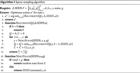
The optimal cost over the sub-MDP is $V_b^{*}(s)={\text{min}}_{\pi }{V}_b^{\pi }(S)$. The approximation algorithm computes an estimate ${\widehat{V}}_b^{*}\left(s_0\right)$ of the optimal $V_b^{*}\left(s_0\right)$ by performing a sampling of the sub-MDP in the neighborhood of s₀. In Algorithm 1 we provide a pseudo-code of the approximation algorithm that was adapted for SDDS. The algorithm requires the SDDS, the set of actions A, the state s₀, and the parameters that determine the accuracy and computational efficiency, h and c. The parameter h is the finite horizon of the sub-MDP. The parameter c is the number of samples per action. Importantly, the time complexity does not depend on the size of the state space of system. Finally, the Algorithm 1 also requires a noise parameter g. The role of the noise is to make the system ergodic.

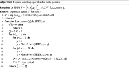
The approximation algorithm can be adapted to cyclic interventions in which actions have a duration period of L steps, and are followed by a recovery period (without intervention) of W-L steps (Yousefi and Dougherty, 2014; Shmulevich and Dougherty, 2010). These type of interventions not only simulate more realistic therapeutic scenarios but result in methods that are computationally less expensive, as the number of considered policies are smaller than the number of policies in which actions can change every time step. For the cyclic intervention, every decision epoch consists of W steps. The approximation algorithm then creates a sub-MDP of h decision epochs by sampling the neighborhood of s₀. The total expected cost for this sub-MDP under a policy π is

$$V_{W,h}^{\pi }\left(s_0\right)=E\left[\sum _{k=0}^{b-1}{\gamma }^{kW}{\tilde{C}}_W\left(s_k,a\right)\right]$$

where ${\tilde{C}}_W\left(s_k,a\right)=E_{s^{\prime }}\left[C_W\left(s_k,a,s^{\prime }\right)\right]$ is the expected cost over a period W starting at state s_k under action a, and $C_W\left(s_k,a,s^{\prime }\right)=L{C}_a+C_{s^{\prime }}$. Similar to the general case, the approximation computes an estimate of the optimal policy that generate the minimum possible $V_{W,b}^{\pi }\left(s_0\right)$. In Algorithm 3 we provide a pseudo-code of the approximation algorithm adapted to cyclic policies.

3. Results and Applications

To test the efficiency and accuracy of our methods we applied them in published models of different sizes. The size of the test models are 6, 16, and 60 nodes. For the small network (with 6 nodes) we computed the exact control policy for the system. Then we used the approximation algorithm to compute an approximated policy for states of interest to compare it with the exact optimal policy obtained by value iteration. For the larger networks, only the approximated policy was computed and then we performed simulations to validate the effectiveness of the approximated policies.

3.1. T-LGL model

Cytotoxic T-cells are part of the immune system that fight against antigens by killing cancer cells and then going through controlled cell death (apoptosis) themselves. The T-cell large granular lymphocyte (T-LGL) leukemia is a disease where cytotoxic T-cells escape apoptosis and keep proliferating. A Boolean network model for this system has been built in (Zhang et al., 2008), and subsequently, steady state analysis for control targets identification has been performed in (Saadatpour et al., 2011; Zañudo and Albert, 2015). This network has 60 nodes; the update functions can be found in the following GitHub site: https://github.com/boaguilar/SDDScontrol.

In order to exhibit an exact control policy we first use a reduced version of the 60-node model (see Figure 1) that was given in (Saadatpour et al., 2011). The reduced network considers the following nodes:

$$\begin{array}{lll}{x}_1=S1P,\hfill & x_2=\mathit{\text{FLIP}},\hfill & x_3=Fas,\hfill \\ x_4=\mathit{\text{Ceramide}},\hfill & x_5=\mathit{\text{DISC}},\hfill & x_6=\mathit{\text{Apoptosis}}.\hfill \end{array}$$

$$\begin{array}{lll}{f}_1=\overline{x_4}\wedge \overline{x_6},\hfill & f_2=\overline{x_5}\wedge \overline{x_6},\hfill & f_3=\overline{x_1}\wedge \overline{x_6,}\hfill \\ f_4=x_3\wedge \overline{x_1}\wedge \overline{x_6},\hfill & f_5=\left(x_4\vee \left(x_3\wedge \overline{x_2}\right)\right)\vee \overline{x_6},\hfill & f_6=x_5\vee x_6.\hfill \end{array}$$

Figure 1:

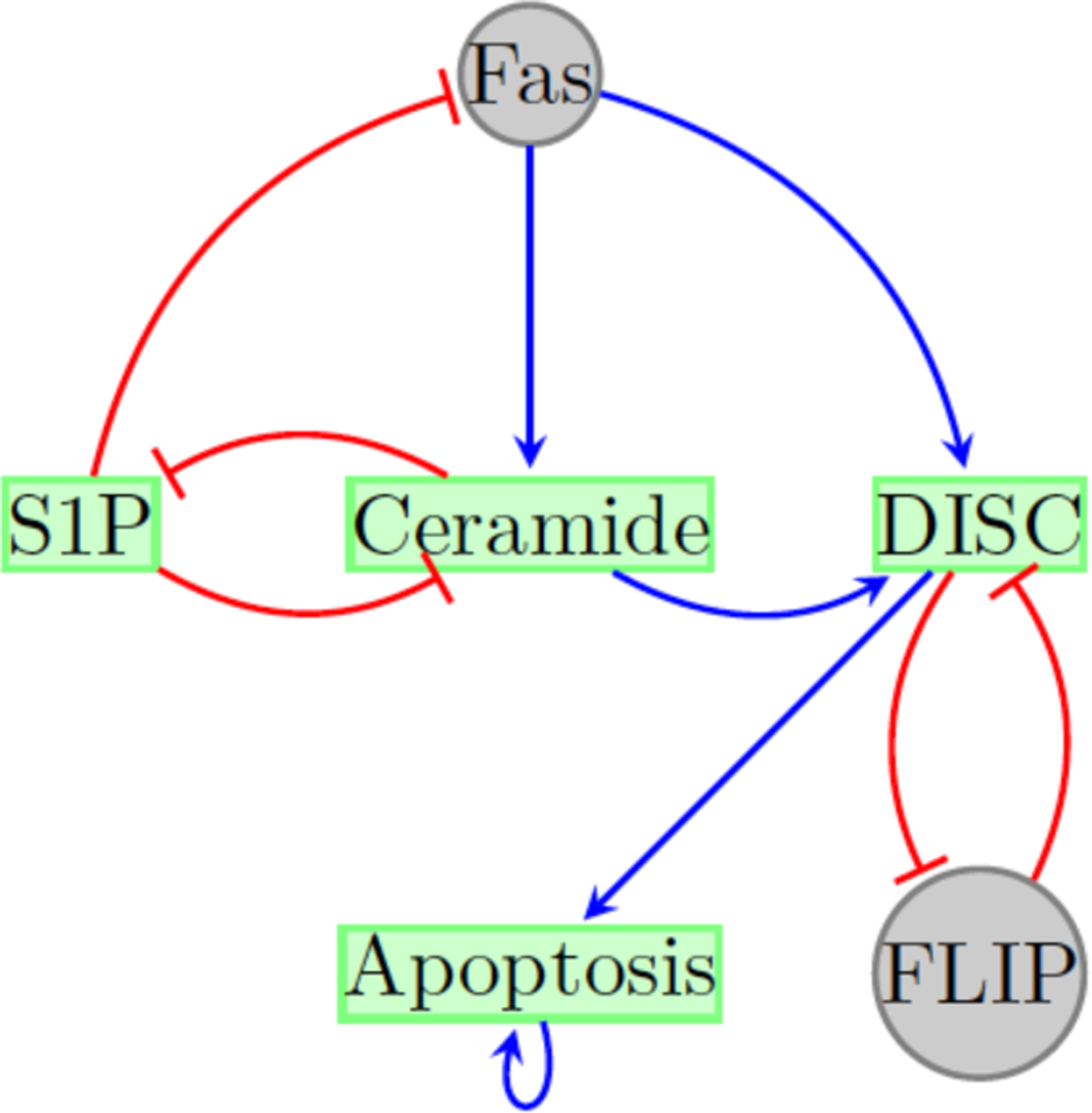
Reduced T-LGL network adapted from (Saadatpour et al., 2011). Control nodes (in gray) represent the deletion of FLIP (FLIP = OFF or x₂ = 0) and the constant expression of Fas (Fas = ON or x₃ = 1).

This reduced T-LGL system has two steady states, one that represents the normal state, 000001, where Apoptosis is ON and the other, 110000, that represents the disease state, where Apoptosis is OFF.

We used the method given in (Murrugarra et al., 2016) to identify control targets in this network that can stabilize the system in a desirable steady state. Here, we consider the controls that represent the deletion of FLIP (FLIP = OFF or x₂ = 0) and the constant expression of Fas (Fas = ON or x₃ = 1). Simultaneous application of these controls will result in the fixed point 001001 that is globally reachable. Note that this new fixed point has x₆ = 1 which means that Apoptosis is ON and thus we can use this fixed point as a desirable state. Using these controls we computed an optimal control policy for the system. Since we have two controls, there are four possible actions: 00 (no intervention), 01 (deletion of FLIP), 10 (constant expression of Fas), and 11 where both controllers are needed (x₂ = 0 and x₃ = 1). Figure 2 shows the control policy where transitions are marked by colors, arrows in green mean no control, arrows in blue represent the control of the node FLIP (x₂ = 0), arrows in orange represent the control of the node Fas (x₃ = 1), and the arrows in red represent the control of both controls. Notice that in Figure 2 only few states require intervention. Especially, the disease state 110000 and the states that were in the synchronous basin of attraction. Also in Figure 2 notice that the controls are only needed transiently, for one step, and then no control is required to direct the system into the desired fixed point.

Figure 2:

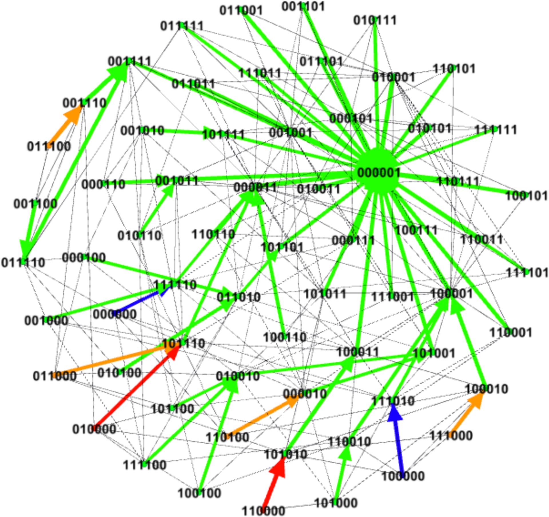
Optimal control policy for the reduced T-LGL network obtained by value iteration. Two controls have been considered, FLIP = OFF (x₂ = 0) and Fas = ON (x₃ = 1). Arrows in green represent no control, arrows in blue represent the control of the node FLIP (x₂ = 0), arrows in orange represent the control of the node Fas (x₃ = 1), and the arrows in red represent the control of both nodes. The colored thick arrows show the most likely transition while arrows in gray represent other possible transitions.

To test the effectiveness of our method, we applied the approximation algorithm for the disease state, 110000, of the reduced network. Figure 3 shows that we our method recovers the exact policy with high probability. Notice that as the parameter h increases the accuracy of the prediction improves.

Figure 3:

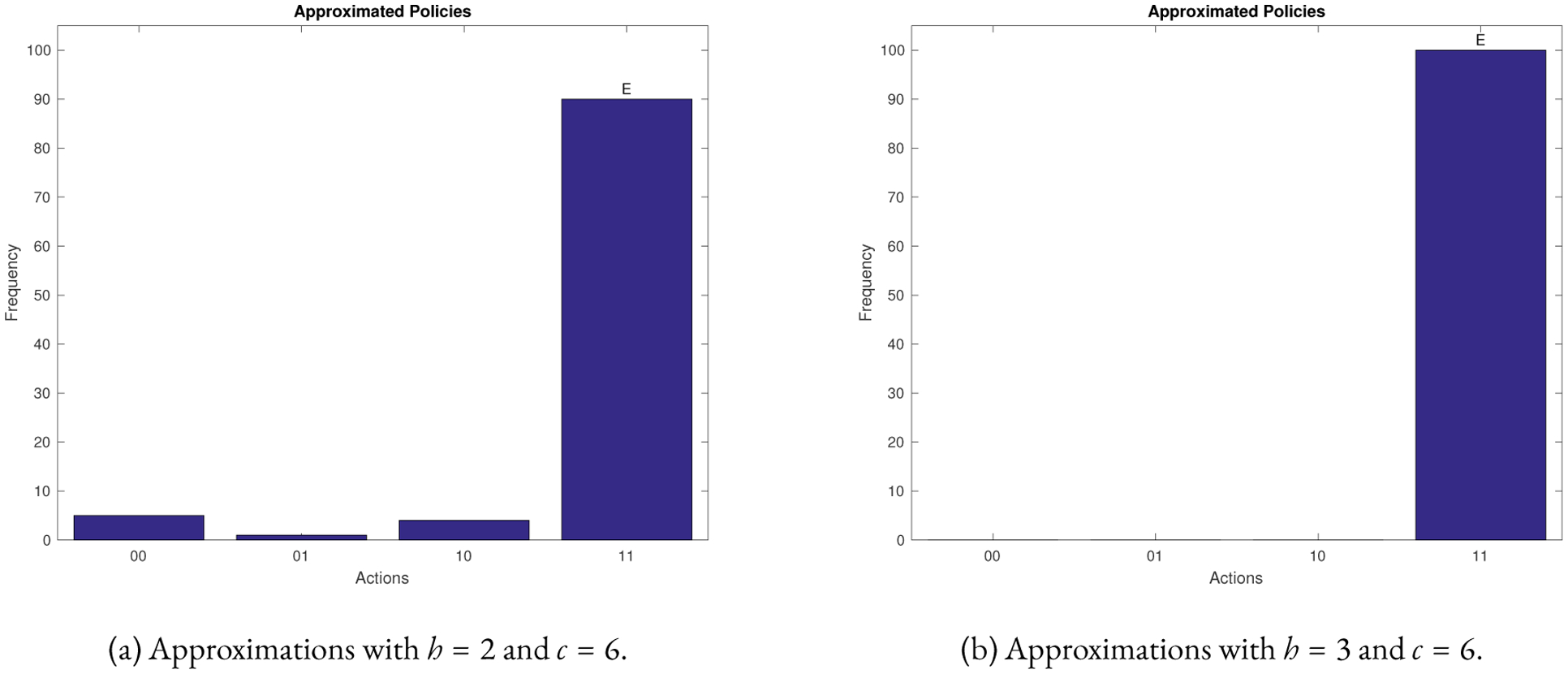
Statistics from using the approximation algorithm for the 6 nodes T-LGL network for the state 110000. Algorithm 1 was used 100 times. The vertical axis shows the frequency of control actions predicted by the approximation algorithm. The horizontal axis shows all possible control actions.

For the model with 60 nodes, we can no longer calculate the exact optimal control policy. The state space of this system has a size of 2⁶⁰ = 1.1529 × 10¹⁸. Thus, we only use the approximation method for this case. By simulation we identified a (synchronous) limit cycle of length 4 and a fixed point, see Table 1. The limit cycle represents the disease state (where Apoptosis is OFF) while the fixed point the normal state (where Apoptosis in ON).

Table 1:

States of the synchronous 4-cycle and the fixed point for the 60 nodes T-LGL network. The bits in bold correspond to the expression level of the node Apoptosis. Thus, the periodic cycle corresponds to the disease state (where Apoptosis is OFF) and the fixed point corresponds to the normal cell state where apoptosis is ON.

States	Binary Expression
Cycle state	111111011101111110110010110101001110110100011010101111110100
Cycle state	101111011101111110110010110101001110110100011010101111110100
Cycle state	001111011101111110110010110101001110110100011010101111110100
Cycle state	011111011101111110110010110101001110110100011010101111110100
Fixed point	000000000000000000000000000000000000001000000000010000110100

For the model with 60 nodes, we also used the same control actions that we used for the reduced model. That is, we considered the controls that represent the deletion of FLIP (FLIP = OFF or x₄₄ = 0) and the constant expression of Fas (Fas = ON or x₃₉ = 1). Simultaneous application of these controls will result in a new fixed point (given in the last row of Table 2) that has x₅₀ = 1 which means that Apoptosis is ON and thus we can use this fixed point as a desirable state. We applied the approximated algorithm (Algorithm 3) for each state (see Table 1) in the limit cycle with the goal of driving the system away from this cycle. Figure 4 shows the statistics after 100 runs of the approximation algorithm for one of states (the third cycle state in Table 1) of the limit cycle, namely, the following state,

$$001111011101111110110010110101001110110100011010101111110100$$ (3)

Table 2:

Simulations from the states of the limit cycle for the 60 nodes T-LGL network. The first column indicates an achieved path under control. The control policy is the same as in the small example. That is, in all cases the system escapes the disease attractor (see Table 1) and converges to a new fixed point given by the controls.

States	Binary Expression
Cycle state	111111011101111110110010110101001110110100011010101111110100
Next state	101111011101111110110010110101001110111101001010101111110100
Next state	001111011101111110110010110101001110111101101010001111110100
Next state	011111011101111110110010110101001110111101101110011111110100
Fixed point	000000000000000000000000000000000000001000000000010000110100
Cycle state	101111011101111110110010110101001110110100011010101111110100
Next state	001111011101111110110010110101001110111101001010101111110100
Next state	011111011101111110110010110101001110111101101010001111110100
Next state	111111011101111110110010110101001110111101101110011111110100
Fixed point	000000000000000000000000000000000000001000000000010000110100
Cycle state	001111011101111110110010110101001110110100011010101111110100
Next state	011111011101111110110010110101001110111101001010101111110100
Next state	111111011101111110110010110101001110111101101010001111110100
Next state	101111011101111110110010110101001110111101101110011111110100
Fixed point	000000000000000000000000000000000000001000000000010000110100
Cycle state	001111011101111110110010110101001110110100011010101111110100
Next state	011111011101111110110010110101001110111101001010101111110100
Next state	111111011101111110110010110101001110111101101010001111110100
Next state	101111011101111110110010110101001110111101101110011111110100
Fixed point	000000000000000000000000000000000000001000000000010000110100

Figure 4:

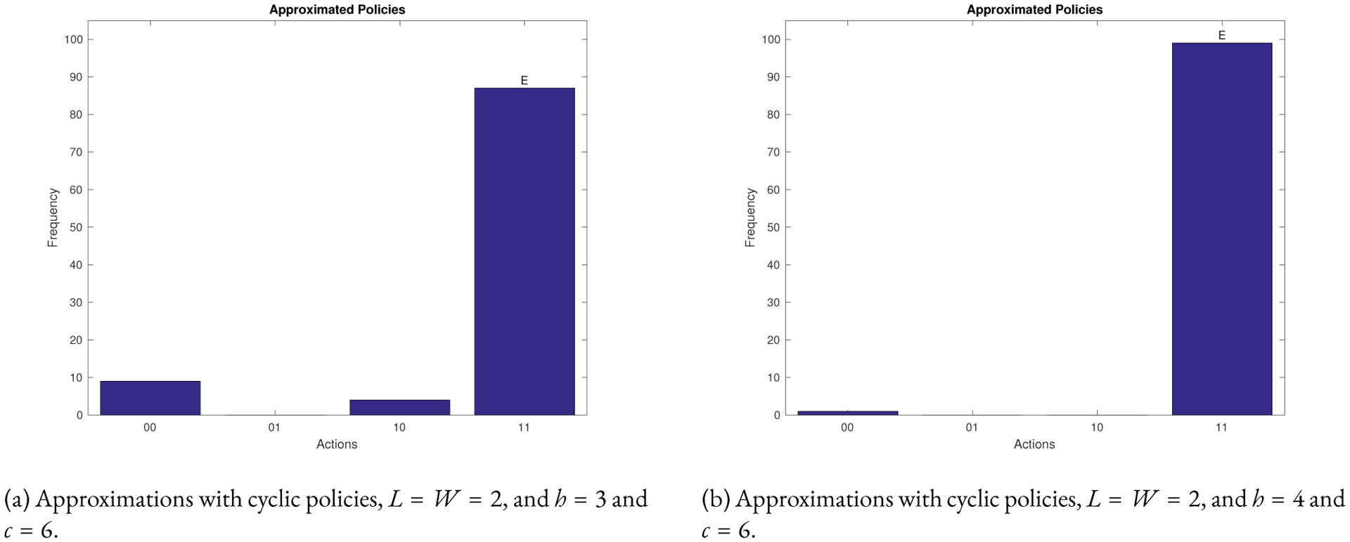
Statistics from using the approximation algorithm for the 60 nodes T-LGL network for the state in Equation 3. Algorithm 3 was used 100 times. The vertical axis shows the frequency of control actions predicted by the approximation algorithm. The horizontal axis show all possible control actions. The simulations contain noise of p=0.05.

Figure 4 shows that we get the policy 11 with high probability. That is, we need both controls. We also get the same control policy with high probability for the other cycle states (data not shown). To test the effectiveness of the high probability policy in Figure 4 we simulated the system from the cycle states in Table 1.

3.1.1. P53-mdm2 network

The tumor suppressor protein p53 can induce cycle arrest or apoptosis in the presence of DNA damage (Geva-Zatorsky et al., 2006; Alon, 2019). A Boolean network model that reproduces the known biology for this system has been built in (Choi et al., 2012). This network considers the following nodes:

$$\begin{array}{llll}{x}_1=ATM,\hfill & x_2=p\mathit{53},\hfill & x_3=Mdm\mathit{2},\hfill & x_4=\mathit{\text{MdmX}},\hfill \\ x_5=Wip\mathit{1},\hfill & x_6=\mathit{\text{cyclinG}},\hfill & x_7=\mathit{\text{PTEN}},\hfill & x_8=p\mathit{21},\hfill \\ x_9=AKT,\hfill & x_{10}=\mathit{\text{cyclinE}},\hfill & x_{11}=Rb,\hfill & x_{12}=E\mathit{2}F1,\hfill \\ x_{13}=p14ARf,\hfill & x_{\mathit{14}}=Bcl\mathit{2},\hfill & x_{15}=Bax,\hfill & x_{16}=\mathit{\text{caspase}}.\hfill \end{array}$$

The update functions for this model are provided at Github site https://github.com/boaguilar/SDDScontrol. We note that the state space for this system has 2¹⁶ = 65536 states.

In the presence of DNA damage the system has a unique (synchronous) limit cycle of length 7. The states of this limit cycle are given in the first row of Table 3. Using the algebraic methods in (Murrugarra et al., 2016), we identified control edges for this network that stabilize the system in a (desired) fixed point. That is, deleting all these edges from the wiring diagram will result in a system that has a single fixed point y₀ that is globally reachable (Murrugarra et al., 2016). The new fixed point y₀ is given in Equation 4. The control targets consist of 9 control edges that are given in the first column of Table 3.

Table 3:

Control policy for the 7 states of the limit cycle in the p53-mdm2 network. The first column has the 9 control edges that allow to redirect the whole system towards the desired fixed point y₀ given in Eq. 4. Columns 2–4 give the control edges identified by the approximation algorithm (Algorithm 3) for the states of the limit cycle. Edges in red indicate common controls for the states in limit cycle. Figure 5 shows simulation results using these control policies.

All States	States of Limit Cycle
	0111110110110100
216 = 65536	1101010011110100	1010010011010100	0011010010010100
possible states.	1101110111110100	1000010011010100	0011110110010100
Edge controls	Edge controls	Edge controls	Edge controls
mdm2 → p53	p53 → Wip1	mdm2 → p53	p53 → Wip1
p53 → Wip1	p21 → Caspase	p53 → Wip1	mdm2 → p21
mdm2 → p21	mdmx → p53	p21 → Caspase	p21 → Caspase
p21 → Caspase	Bcl2 → Bax	Bcl2 → Bax	mdmx → p53
ATM → Rb			Bcl2 → Bax
mdm2 → Rb
mdmx → p53
Rb → E2F1
Bcl2 → Bax

$$y_0=(1,1,1,0,0,1,0,1,1,0,0,1,0,0,1,1),$$ (4)

We note that the state in Equation 4 represents cell death, where x₂ = p53 and x₁₆ = caspase are ON. Thus, we used this fixed point as a desired state for our control objective.

We applied the approximation algorithm (Algorithm 3) using a cyclic policy with L = W = 5, and h = 2 and c = 3 for each state in the limit cycle. After 100 runs of Algorithm 3, we obtained (with high probability) the control policies given in Table 3. In columns 2–4 of Table 3 we group the states that have the same control policy.

To validate the effectiveness of the control policies given in Table 3, we performed simulations starting from each state of the limit cycle using the control policies given in columns 2–4 of Table 3. The results of these simulations are given in Figure 5. Figure 5 shows that the estimated policies are effective as it is possible to get to the desired fixed point y₀ given in Equation 4 from each state of the limit cycle. The simulations were performed using the parameters specified in the caption of Figure 5.

Figure 5:

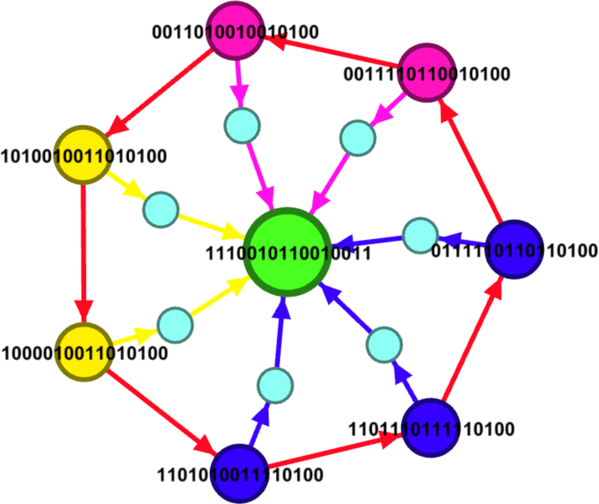
Simulations using the control policies given in Table 3 for the states of the limit cycle of the p53-mdm2 network. For each cycle state, we applied the control edges given in columns 2–4 of Table 3. The smaller intermediate nodes indicate that the controls have been applied twice, for 5 steps each time. The colors indicate the different policies indicated in Table 3. Nodes with the same color have the same control policy as specified in Table 3.

4. Discussion and Conclusions

Finding optimal intervention strategies for GRN is an important problem in computational biology. Intervention strategies consisting of combinations of control targets such as the knockout of a gene and the disruption of an interaction are becoming more and more relevant (Lee et al., 2012; Choi et al., 2012; Erler and Linding, 2012; Zañudo et al., 2017). The problem of computing a control policy that dictates what intervention to apply at each state of a system becomes computational prohibitive for large networks (e.g., networks with more than 20 nodes). This paper focuses on approximation techniques based on Monte Carlo sampling of the transition probabilities of generative models. More specifically, in this paper we provide approximation algorithms to estimate the optimal control policy for a discrete stochastic system. The complexity of the proposed algorithms does not depend on the size of the state space of the system, it only depends on the sampling size and the depth of the iterations. This feature makes the proposed algorithms efficient and they can be applied to a large GRN. Importantly, it can be shown that the approximation method that we used in this paper provides a good estimate function (or near optimal function) to the optimal cost function as was shown for general generative models in (Kearns et al., 2002).

Approximation techniques are useful when trying to compute a control policy for a large system. There are algorithms to calculate optimal control policies (Abul et al., 2004; Datta et al., 2004; Pal et al., 2006; Yousefi et al., 2012; Chen et al., 2012) but the computational complexity of these algorithms, which is at least exponential in the size of the state space, is very high. For instance, for the 60 nodes model that was discussed in the results section, the state space has 2⁶⁰ = 1.1529 × 10¹⁸ states. Thus, it becomes unfeasible to calculate an exact control policy for this system. The approximation technique that was used in this paper was very efficient for this model.

The methods presented in this paper were validated using a T-LGL network of 60 nodes and a network for the p53-mdm2 system of 16 nodes. The T-LGL system has two attractors, a limit cycle that represents a disease state and a fixed point representing a normal state (apoptosis). The approximation algorithm was applied to calculate a control policy that allows the system to escape from the disease state and directs the system towards the desired fixed with high probability. Likewise, for the p53-mdm2 system, the approximation algorithm successfully generates a control policy that drives the system towards a desired fixed point.

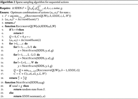
For our applications, we used Algorithm 1 and 3 and these can be modified to incorporate more realistic control strategies considering a number of steps for recovery such as the cyclic and acyclic interventions that was considered in (Yousefietal., 2012). We can also adapt our approximation algorithms for sequential interventions such as the interventions strategies described in (Lee et al., 2012), where the order of the control actions to be applied matters. Algorithm 2 provides a pseudocode for sequential interventions for SDDS. Moreover, the methods developed in this paper can be applied to multistate discrete models of GRN (Sordo Vieira et al., 2019; Veliz-Cuba et al., 2010) and Probabilistic Boolean Networks PBN (Shmulevich et al., 2002). Finally, the approximation method is suitable for a planning strategy, in which simulations are performed under control; the method is applied to every state attained.

We remark that the efficiency of the method depends on the topology of the network, particularly on the maximum in-degree. For instance, the T-LGL model of 60 nodes has a maximum in-degree of 7 while the p53 network of 16 nodes has a maximum in-degree of 10. Although the T-LGL network is larger than the p53 network, it has a smaller maximum in-degree. As a result, the approximation algorithm was more efficient for the 60-node model than for the 16-node model. Also, the noise added to the system (see Section 2.5) can affect the efficiency of the algorithm. In large systems such as the T-TLG network, the noise can make the system to jump into a random state and it might take a large number of steps to get to the desired target state. The noise is not required for controllable systems, where every state is reachable under the control.

Finally, we implemented the proposed control algorithms in C++ and our code is freely available through the following GitHub website: https://github.com/boaguilar/SDDScontrol. This website also contains the associated files of the examples discussed in this paper.

References

- Abou-Jaoudé W, Traynard P, Monteiro PT, Saez-Rodriguez J, Helikar T, Thieffry D, and Chaouiya C (2016). Logical modeling and dynamical analysis of cellular networks. Front Genet 7, 94. 67 [DOI] [PMC free article] [PubMed] [Google Scholar]
- Abul O, Alhaj R, and Polat F (2004). Markov decision processes based optimal control policies for probabilistic boolean networks. In Bioinformatics and Bioengineering, 2004. BIBE 2004. Proceedings. Fourth IEEE Symposium on, pp. 337–344. IEEE. 68, 78 [Google Scholar]
- Alon U (2019). An Introduction to Systems Biology: Design Principles of Biological Circuits (Second ed.). Chapman and Hall/CRC Computational Biology Series. 67, 75 [Google Scholar]
- Bertsekas DP (2005). Dynamic Programming and Optimal Control. Athena Scientifik. 68, 71 [Google Scholar]
- Bertsekas DP (2019). Reinforcement Learning and Optimal Control. Athena Scientific. 68 [Google Scholar]
- Chang H, Hu J, Fu M, and Marcus S (2013). Simulation-Based Algorithms for Markov Decision Processes (Second ed.). Springer. 68 [Google Scholar]
- Chen X, Jiang H, Qiu Y, and Ching W-K (2012). On optimal control policy for probabilistic boolean network: a state reduction approach. BMC Systems Biology 6(Suppl 1), S8. 68, 78 [DOI] [PMC free article] [PubMed] [Google Scholar]
- Choi M, Shi J, Jung SH, Chen X, and Cho K-H (2012). Attractor landscape analysis reveals feedback loops in the p53 network that control the cellular response to dna damage. Sci. Signal 5(251), ra83. 70, 75, 78 [DOI] [PubMed] [Google Scholar]
- Datta A, Choudhary A, Bittner ML, and Dougherty ER (2004). External control in markovian genetic regulatory networks: the imperfect information case. Bioinformatics 20(6), 924–930. 68, 78 [DOI] [PubMed] [Google Scholar]
- Erler JT and Linding R (2012, May). Network medicine strikes a blow against breast cancer. Cell 149(4), 731–3. 78 [DOI] [PubMed] [Google Scholar]
- Fall CP, Marland AS, Wagner JM, and Tyson JJ (2010). Computational Cell Biology (Interdisciplinary Applied Mathematics). Springer. 67 [Google Scholar]
- Geva-Zatorsky N, Rosenfeld N, Itzkovitz S, Milo R, Sigal A, Dekel E, Yarnitzky T, Liron Y, Polak P, Lahav G, and Alon U (2006). Oscillations and variability in the p53 system. Mol Syst Biol 2, 2006.0033. 75. [DOI] [PMC free article] [PubMed] [Google Scholar]
- Gillespie DT (1977). Exact stochastic simulation of coupled chemical reactions. The Journal of Physical Chemistry 81(25), 2340–2361. 67 [Google Scholar]
- Helikar T, Kochi N, Kowal B, Dimri M, Naramura M, Raja SM, Band V, Band H, and Rogers JA (2013). A comprehensive, multi-scale dynamical model of erbb receptor signal transduction in human mammary epithelial cells. PLoS One 8(4), e61757. 68 [DOI] [PMC free article] [PubMed] [Google Scholar]
- Helikar T, Konvalina J, Heidel J, and Rogers JA (2008, Feb). Emergent decision-making in biological signal transduction networks. Proc Natl Acad Sci U S A 105(6), 1913–8. 68 [DOI] [PMC free article] [PubMed] [Google Scholar]
- Huang S (1999, Jun). Gene expression profiling, genetic networks, and cellular states: an integrating concept for tumorigenesis and drug discovery. J Mol Med (Berl) 77(6), 469–80. 67 [DOI] [PubMed] [Google Scholar]
- Huang S, Ernberg I, and Kauffman S (2009, Sep). Cancer attractors: a systems view of tumors from a gene network dynamics and developmental perspective. Semin Cell Dev Biol 20(7), 869–76. 67 [DOI] [PMC free article] [PubMed] [Google Scholar]
- Kauffman S, Peterson C, Samuelsson B, and Troein C (2003). Random Boolean network models and they east transcriptional network. Proceedings of the National Academy of Sciences 100(25), 14796–14799. 67 [DOI] [PMC free article] [PubMed] [Google Scholar]
- Kauffman SA (1969, Mar). Metabolic stability and epigenesis in randomly constructed genetic nets. J Theor Biol 22(3), 437–67. 67 [DOI] [PubMed] [Google Scholar]
- Kazemzadeh L, Cvijovic M, and Petranovic D (2012). Boolean model of yeast apoptosis as a tool to study yeast and human apoptotic regulations. Front Physiol 3, 446. 68 [DOI] [PMC free article] [PubMed] [Google Scholar]
- Kearns MJ, Mansour Y, and Ng AY (2002). A sparse sampling algorithm for near-optimal planning in large markov decision processes. Machine Learning 49(2–3), 193–208. 68, 71, 78 [Google Scholar]
- Lee MJ, Ye AS, Gardino AK, Heijink AM, Sorger PK, MacBeath G, and Yaffe MB (2012, May). Sequential application of anticancer drugs enhances cell death by rewiring apoptotic signaling networks. Cell 149(4), 780–94. 78 [DOI] [PMC free article] [PubMed] [Google Scholar]
- Madrahimov A, Helikar T, Kowal B, Lu G, and Rogers J (2013, Jun). Dynamics of influenza virus and human host interactions during infection and replication cycle. Bull Math Biol 75(6), 988–1011. 68 [DOI] [PubMed] [Google Scholar]
- Murrugarra D and Dimitrova ES (2015, Dec). Molecular network control through boolean canalization. EURASIP J Bioinform Syst Biol 2015(1), 9. 69, 70 [DOI] [PMC free article] [PubMed] [Google Scholar]
- Murrugarra D, Miller J, and Mueller AN (2016). Estimating propensity parameters using google pagerank and genetic algorithms. Front Neurosci 10, 513. 68 [DOI] [PMC free article] [PubMed] [Google Scholar]
- Murrugarra D, Veliz-Cuba A, Aguilar B, Arat S, and Laubenbacher R (2012). Modeling stochasticity and variability in gene regulatory networks. EURASIP Journal on Bioinformatics and Systems Biology 2012(1), 5. 67, 68 [DOI] [PMC free article] [PubMed] [Google Scholar]
- Murrugarra D, Veliz-Cuba A, Aguilar B, and Laubenbacher R (2016, Sep). Identification of control targets in boolean molecular network models via computational algebra. BMC Syst Biol 10(1), 94. 68, 69, 70, 74, 77 [DOI] [PMC free article] [PubMed] [Google Scholar]
- Naseem M, Philippi N, Hussain A, Wangorsch G, Ahmed N, and Dandekar T (2012, May). Integrated systems view on networking by hormones in arabidopsis immunity reveals multiple crosstalk for cytokinin. Plant Cell 24(5), 1793–814. 68 [DOI] [PMC free article] [PubMed] [Google Scholar]
- Pal R, Datta A, and Dougherty ER (2006). Optimal infinite-horizon control for probabilistic boolean networks. IEEE Transactions on Signal Processing 54(6–2), 2375–2387. 68, 78 [Google Scholar]
- Raza S, Robertson KA, Lacaze PA, Page D, Enright AJ, Ghazal P, and Freeman TC (2008). A logic-based diagram of signalling pathways central to macrophage activation. BMC Syst Biol 2, 36. 68 [DOI] [PMC free article] [PubMed] [Google Scholar]
- Saadatpour A, Wang R-S, Liao A, Liu X, Loughran TP, Albert I, and Albert R (2011, Nov). Dynamical and structural analysis of at cell survival network identifies novel candidate therapeutic targets for large granular lymphocyte leukemia. PLoS Comput Biol 7(11), e1002267. 68, 73, 74 [DOI] [PMC free article] [PubMed] [Google Scholar]
- Saez-Rodriguez J, Simeoni L, Lindquist JA, Hemenway R, Bommhardt U, Arndt B, Haus U, Weismantel R, Gilles ED, Klamt S, and Schraven B (2007). A logical model provides insights into T cell receptor signaling. PLoS Computational Biology 3(8). 68. [DOI] [PMC free article] [PubMed] [Google Scholar]
- Samaga R, Saez-Rodriguez J, Alexopoulos LG, Sorger PK, and Klamt S (2009, Aug). The logic of egfr/erbb signaling: theoretical properties and analysis of high-throughput data. PLoS Comput Biol 5(8), e1000438. 68 [DOI] [PMC free article] [PubMed] [Google Scholar]
- Shmulevich I and Dougherty ER (2010). Probabilistic Boolean Networks - The Modeling and Control of Gene Regulatory Networks. SIAM. 72 [Google Scholar]
- Shmulevich I, Dougherty ER, Kim S, and Zhang W (2002). Probabilistic boolean networks: a rule-based uncertainty model for gene regulatory networks. Bioinformatics 18(2), 261–274. 67, 78 [DOI] [PubMed] [Google Scholar]
- Singh A, Nascimento JM, Kowar S, Busch H, and Boerries M (2012, Sep). Boolean approach to signalling pathway modelling in hgf-induced keratinocyte migration. Bioinformatics 28(18), i495–i501. 68 [DOI] [PMC free article] [PubMed] [Google Scholar]
- Sordo Vieira L, Laubenbacher RC, and Murrugarra D (2019, Dec). Control of intracellular molecular networks using algebraic methods. Bull Math Biol 82(1), 2. 68, 78 [DOI] [PMC free article] [PubMed] [Google Scholar]
- Sutton RS and Barto AG (1998). Reinforcement learning: An introduction, Volume 1. MIT press Cambridge. 68, 71 [Google Scholar]
- Thomas R and D’Ari R (1990). Biological feedback. Boca Raton: CRC Press. 67 [Google Scholar]
- Tomas H and et al. The cell collective. 68 [Google Scholar]
- Veliz-Cuba A, Jarrah AS, and Laubenbacher R (2010, Jul). Polynomial algebra of discrete models in systems biology. Bioinformatics 26(13), 1637–43. 78 [DOI] [PubMed] [Google Scholar]
- Yousefi MR, Datta A, and Dougherty ER (2012). Optimal intervention strategies for therapeutic methods with fixed-length duration of drug effectiveness. Signal Processing, IEEE Transactions on 60(9), 4930–4944. 68, 70, 71, 78 [Google Scholar]
- Yousefi MR and Dougherty ER (2014). A comparison study of optimal and suboptimal intervention policies for gene regulatory networks in the presence of uncertainty. EURASIP Journal on Bioinformatics and Systems Biology 2014(1), 6–6. 72 [DOI] [PMC free article] [PubMed] [Google Scholar]
- Zañudo JGT and Albert R (2015, Apr). Cell fate reprogramming by control of intracellular network dynamics. PLoS Comput Biol 11(4), e1004193. 68, 74 [DOI] [PMC free article] [PubMed] [Google Scholar]
- Zañudo JGT, Yang G, and Albert R (2017, 07). Structure-based control of complex networks with nonlinear dynamics. Proc Natl Acad Sci U S A 114(28), 7234–7239. 68, 78 [DOI] [PMC free article] [PubMed] [Google Scholar]
- Zhang R, Shah MV, Yang J, Nyland SB, Liu X, Yun JK, Albert R, and Loughran TP Jr (2008, Oct). Network model of survival signaling in large granular lymphocyte leukemia. Proc Natl Acad Sci U S A 105(42), 16308–13. 68, 74 [DOI] [PMC free article] [PubMed] [Google Scholar]