

Abstract
Motivation
The overall association evidence of a genetic variant with multiple traits can be evaluated by cross-phenotype association analysis using summary statistics from genome-wide association studies. Further dissecting the association pathways from a variant to multiple traits is important to understand the biological causal relationships among complex traits.
Results
Here, we introduce a flexible and computationally efficient Iterative Mendelian Randomization and Pleiotropy (IMRP) approach to simultaneously search for horizontal pleiotropic variants and estimate causal effect. Extensive simulations and real data applications suggest that IMRP has similar or better performance than existing Mendelian Randomization methods for both causal effect estimation and pleiotropic variant detection. The developed pleiotropy test is further extended to detect colocalization for multiple variants at a locus. IMRP will greatly facilitate our understanding of causal relationships underlying complex traits, in particular, when a large number of genetic instrumental variables are used for evaluating multiple traits.
Availability and implementation
The software IMRP is available at https://github.com/XiaofengZhuCase/IMRP. The simulation codes can be downloaded at http://hal.case.edu/∼xxz10/zhu-web/ under the link: MR Simulations software.
Supplementary information
Supplementary data are available at Bioinformatics online.
1 Introduction
In the past decade, genome-wide association studies (GWASs) have been successful in identifying genetic variants associated with complex traits (https://www.genome.gov/gwastudies/). Although most GWASs have been conducted for individual traits, a recent study showed that 90% of the identified variants are associated with multiple traits (Watanabe et al., 2019). Such phenomenon is often termed as cross-phenotype (CP) association (Andreassen et al., 2013; Cortes et al., 2020; Cotsapas et al., 2011; Liang et al., 2017; Park et al., 2016; Solovieff et al., 2013; Wagner and Zhang, 2011; Yan et al., 2020; Zhu et al., 2015), which suggests that multiple traits potentially share common genetic pathways. Noted that CP association is not the same as pleiotropy, a concept that has been continuously evolving in light of current genomic data. Solovieff et al. (2013) classified CP associations into four categories: (i) mediated pleiotropy; (ii) biological pleiotropy; (iii) colocalization; and (iv) spurious pleiotropy. Mediated pleiotropy and biological pleiotropy have been called as vertical and horizontal pleiotropy, respectively (Jordan et al., 2019; Verbanck et al., 2018). In brief, mediated pleiotropy occurs when a genetic variant directly affects one trait that in turn has a direct contribution to a second trait. For example, genetic variants are associated with both low-density lipoprotein (LDL) levels and the risk of myocardial infarction, but their associations with myocardial infarction are caused through the variation of LDL levels (Voight et al., 2012). Biological pleiotropy occurs when a genetic variant influences multiple traits through independent physiological mechanisms. Thus, the association of the genetic variant with the second trait does not disappear conditional on the first trait. For example, the rs6983267 variant on 8q24 is a risk factor for both prostate and colorectal cancer by conferring differential in vivo activity to a MYC enhancer in both colon and prostate tissue types (Pomerantz et al., 2009; Wasserman et al., 2010). Colocalization is also considered as a type of pleiotropy, in which multiple risk variants of different traits fall into the same gene or genomic region. GWASs have reported that variants of many traits are colocalized with eQTLs in different tissue types (Barbeira et al., 2018; Giambartolomei et al., 2014; Hormozdiari et al., 2016; Wen et al., 2017). Spurious pleiotropy is caused by various biases including ascertainment bias, phenotypic misclassification and shared controls (Solovieff et al., 2013). The CP association analysis can greatly improve statistical power in detecting genetic variants associated with multiple traits (Turley et al., 2018; Zhu et al., 2015), but it does not provide information on the underlying pleiotropy type. Novel statistical approaches are necessary to differentiate different pleiotropies for better understanding of causal relationships among traits. To simplify our discussion, we call biological (horizontal) pleiotropy as pleiotropy, simplify mediated pleiotropy as mediation, leave colocalization as it is, and do not consider spurious pleiotropy from now on.
Mendelian Randomization (MR) is a widely used epidemiological approach to infer causality of an exposure on a disease outcome (Davey Smith and Hemani, 2014; Evans and Davey Smith, 2015). MR uses mediation genetic variants as instrumental variables (IVs) for testing whether the exposure has a causal role in the etiology of diseases (Burgess et al., 2017). Since the proportion of phenotypic variation explained by a genetic variant is often small, a meta-analysis of the inverse variance weighted (IVW) approach can be applied (Bowden et al., 2015) to combine multiple variants to improve the statistical power in MR analysis. An inherent difficulty of MR lies in the selection of mediation genetic variants as IVs. When IVs consist of genetic variants with pleiotropic effects, MR will lead to a biased estimate of a causal effect (Bowden et al., 2015). In fact, there is a debate about whether MR can reliably identify causality between two traits given the widespread of pleiotropy or colocalization (Davey Smith, 2015; Pickrell, 2015). To correct the potential bias from variants with pleiotropic effect, MR-Egger regression has been developed without the need to identify any pleiotropic variants, however the power is also diminished (Bowden et al., 2015). Recently, MR Pleiotropy RESidual Sum and Outlier (MR-PRESSO) approach has been developed to detect pleiotropic outliers in multi-instrument summary-level MR analysis and the causal effect estimate is obtained using the IVW approach after excluding the outliers (Verbanck et al., 2018). However, MR-PRESSO requires a simulation procedure to test pleiotropy, which substantially increases computational cost. Similarly, the generalized summary data-based MR (GSMR) approach detects pleiotropic variants and performs MR analysis after dropping the pleiotropic variants (Zhu et al., 2018). In particular, GSMR chooses the single nucleotide polymorphism (SNP) that shows the strongest association with the exposure in the third quantile of the distribution. A different approach based on parametric mixture model (MRmix) has recently been developed by assuming bivariate effect-size distribution of the SNPs across pairs of traits (Qi and Chatterjee, 2019). Under the zero modal pleiotropy assumption (ZEMPA), MRmix showed a better trade-off between bias and variance than existing estimators. Similar to MR-Egger, MRmix did not performed well when the number of IVs is small. Further, MRmix does not provide a way to identify pleiotropic loci.
In this study, we introduce the Iterative Mendelian Randomization and pleiotropy (IMRP) approach to overcome shortcomings of existing methods. We model the residual distribution of Γ ^-βγ ^, where Γ ^ and γ ^ represent the effect sizes of an IV for an outcome and an exposure, respectively, and β is the causal effect of the exposure to the outcome. The residual follows a normal distribution when no IVs have pleiotropic effect. IMRP identifies pleiotropic IVs and recalculates causal effect after excluding pleiotropic IVs at each iterative step. Consequently, it can simultaneously perform MR analysis and detect pleiotropic variants. IMRP is computationally efficient as it is based on the IVW method and uses GWAS summary statistics without requiring simulations. We evaluated the performance of IMRP by comparing it with existing MR methods using extensive simulations. We further applied IMRP to publicly available GWAS summary statistics to estimate causal effects and search for pleiotropic loci.
2. Materials and methods
2.1. Introduction of existing MR methods
We assume, there are summary statistics of n independent genetic variants for two traits and being available from GWASs. The summary statistics are either from the same dataset or different datasets (possibly with overlapping samples). We assume that the association paths between genetic variants and two traits (demonstrated in Fig. 1) can be represented by the following models:
| (1) |
where is the direct contribution of the variant to trait , and are the direct contributions of variant to traits and , is the causal effect of trait to trait , U represents confounding factors and and are error terms, respectively. In these two equations, the contribution of a variant (i = 1,…, n1) to trait is mediated through . In contrast, each of (i = 1,…, n2) has a pleiotropic effect. The goal of MR analysis is to establish the causal contribution of the exposure to the outcome by using a set of genetic variants as the IVs. We assume all the genetic variants are independent, which can be achieved by pruning variants. In the MR analysis, a valid IV requires that the genetic variant is (i) independent of U; (ii) associated with exposure ; and (iii) independent of the outcome conditional on the exposure and confounders U.
Fig. 1.
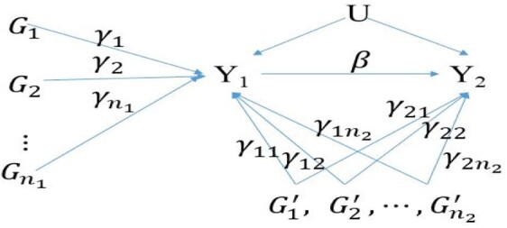
The association paths of genetic IVs, exposure (Y1) and outcome (Y2). represent mediation variants, which are valid IVs in MR analysis. represent pleiotropic variants, which are invalid IVs in MR analysis. Each γ represents a direct contribution of a genetic variant. β represents the causal effect from exposure Y1 to outcome Y2. U represents confounding factors
Let and be the estimated effect sizes of variants and on the exposure , respectively, from the GWAS. Correspondingly, let and be the estimated effect sizes of variants and on the outcome respectively. It is to observe that for the mediation variant , and for the pleiotropic variant . Noted that, the effect size of a pleiotropic variant to the outcome has an additional term besides the effect through the exposure. For an individual IV, the causal effect can be estimated by , which is unbiased if the IV is a mediation variant and biased if the IV is a pleiotropic variant. With multiple IVs, the causal effect estimator can be calculated as the weighted meta-analysis with the weight being the inverse variance of , which refers the IVW estimator (Borenstein, 2009). Alternatively, we can perform a weighted linear regression of the on : . When is fixed to be 0, the weighted least square estimator of is the IVW estimator. Accordingly, the MR-Egger estimator corresponds to the weighted least estimator of without fixing to be 0 (Bowden et al., 2015). Including the variants with pleiotropic effects will lead to a biased estimation of the causal effect. Although such a bias may be alleviated through Egger regression, it has substantially reduced statistical power in testing causality (Bowden et al., 2015). Hence, it is desirable to identify and exclude pleiotropy variants from MR analysis in order to obtain an unbiased estimate of the causal effects, while maintaining statistical power. Thus, MR-PRESSO first identifies horizontal pleiotropic variants and then performs IVW to estimate the causal effect by removing the pleiotropic variants (Verbanck et al., 2018). MR-PRESSO comprises of three steps: (i) testing whether horizontal pleiotropic variants are present through a global test; (ii) performing an outlier test to detect pleiotropic variants; and (iii) comparing the causal estimates before and after removal of pleiotropic variants through a distortion test. The global and pleiotropic variant tests are based on a leave-one out approach with the null distribution is obtained by simulations. Since MR-PRESSO estimates the causal effect after removing potential pleiotropic variants, it is less biased than IVW but is computationally intensive. GSMR shares similarity to MR-PRESSO by identifying pleiotropic variants and performing IVW analysis after excluding the pleiotropic variants without using simulations (Zhu et al., 2018). On the other hand, MRmix is an estimating equation approach that requires the residuals to follow a normal-mixture model (Qi and Chatterjee, 2019). The normal-mixture model seems plausible when the genetic instruments include mediation variants, horizontal pleiotropic variants, as well as the genetic variants contributing to reverse causality. In order to achieve an unbiased causal estimate, MRmix requires the ZEMPA assumption. When the sample size is large, MRmix usually shows a better trade-off between bias and variance than the approaches mentioned before, even more than when 50% IVs are invalid (Qi and Chatterjee, 2019). Similar to MR-Egger, MRmix did not performed well when the number of IVs is small.
2.2. IMRP method
Here, we propose a direct test to differentiate mediation from pleiotropy before MR analysis. The null hypothesis of the test is . When the causal effect is known, the test statistic is
| (2) |
where and are the estimated effect sizes of a variant on and , respectively. The statistic asymptotically follows a standard normal distribution N(0,1) when mediation is true. Under the alternative hypothesis that a variant has a pleiotropic effect, departs from mean 0. The problem of this test is that the causal effect is unknown. To solve this problem, we propose an iterative approach named IMRP by combining the pleiotropy test with MR analysis:
Initialization: selecting n genome-wide significant independent variants of exposure Y1 and obtain the initial causal estimate of by MR-Egger analysis, named as .
Pleiotropy test: for each genetic variant (i=1,…, n) at the iteration, we perform the test using to determine whether the variant has a pleiotropic effect at a predefined significance level α.
Estimation of causal effect : we perform IVW analysis to obtain after removing the variants found to be significant in pleiotropy test at step 2;
Iteration: the above steps 2 and 3 are repeated until there is no change in detected pleiotropic variants.
The initial value at step 1 above can be chosen in different ways. For example, we can also use the causal effect estimate of IVW by including all the IVs. However, taking the MR-Egger estimate as its initial estimate followed by IVW has the advantages of both MR-Egger, which is less biased when pleiotropy is present or Instrument Strength Independent of Direct Effect (InSIDE) assumption is not valid, and IVW, which has less uncertainty, as we observed in simulations. At step 2, let be the estimated causal effect by IVW. The pleiotropy test statistic for a genetic variant is modified as . The denominator variance can be approximated by using the delta method. Here, we ignore the correlation of and and the correlation of and , which is reasonable because is estimated using all independent IVs and less dependent on individual or . When GWAS of Y1 and Y2 are performed in the same sample cohort, is the correlation coefficient of Y1 and Y2. In general, represents the correlation of and induced by overlapping or related samples in the GWASs of Y1 and Y2 and can be estimated using GWAS summary statistics (Zhu et al., 2015) or LD score regression (Bulik-Sullivan et al., 2015).
The presence of pleiotropic variants among the n IVs can be examined by a global test: , which can be approximated as a χ2 distribution with n-1 degrees of freedom for n independent IVs. To test whether an individual variant has a pleiotropic effect, we use at the significance level 0.05/n at the final stage. When a large number of potential IVs are available in the MR analysis, we can use less strict significance level to aggressively exclude IVs with potential pleiotropic effect, as we demonstrated in our real data analysis. IMRP is a combined approach to test pleiotropy versus mediation while performing MR analysis and estimating the causal effect of Y1 on Y2 simultaneously, therefore, it can robustly estimate the causal contribution of a risk factor to an outcome.
The single variant pleiotropy test statistic can be readily extended to multiple variants at a locus. In this case, and are vectors representing the estimated effect sizes from GWAS of M genetic variants at a locus for the outcome and exposure, respectively. Let and . We construct the corresponding statistics of M variants by
| (3) |
where is an variance–covariance matrix with diagonal elements , and off-diagonal elements , where is the linkage disequilibrium (LD) parameter between markers and If we work on the standardized Y1, Y2 and markers, we have and . Further assuming is ignorable in comparing with or , we can simplify to
where is the LD matrix among M variants. Under the null hypothesis of mediation, follows a χ2 distribution with M degrees of freedom. When the variants are in high LD, matrix D can be singular. In this case principle component analysis by Eigen decomposition of the LD matrix can be applied. We choose the number of components that together represent at least 90% of the variance to determine the degree of freedom for the χ2 test.
2.3. Simulations
We conducted simulations to evaluate the type I error and power of IMRP in detecting pleiotropy and to compare the bias of causal effect estimates with the existing MR methods in a variety of scenarios. We compared IMRP with the simulation-based MR-PRESSO because of their similar features in identifying pleiotropic variants. Following the simulation method in Verbanck et al. (2018), we simulated two traits and 50 variants with a variety of proportions of genetic variants with pleiotropic effects. The two traits were simulated with or without causal relationship. We simulated pleiotropy variants and their effects to the two traits with or without satisfying the InSIDE, referring to the condition that the direct effects of the genetic variants , which are and in the model (1), are independent (Bowden et al., 2015). The effect sizes and of genetic variants in model (1) were drawn from a uniform distribution U(0.5,1). If the InSIDE condition is invalid, we added to both and a common value drawn from U(0, 0.1), in order to create the dependence between the pleiotropic effects for both traits. We simulated positive pleiotropy type by drawing all from U(0.5, 1), and balanced pleiotropy type by drawing half of from U(0.5, 1) and the other half from −U(0.5, 1). We varied the causal effect parameter β to be 0, 0.1, 0.2, 0.5 and the percentage of pleiotropic variants to be 0%, 4%, 50% or 90%. We simulated trait and in two cases: (i) both and came from the same cohort (one-sample) and (ii) and came from two independent cohorts (two-samples), with sample size 10 000. We performed linear regression of and on the 50 IVs to obtain the summary statistics of the IVs. To save computational time, we performed the linear regression by including all IVs in the regression model. Therefore, the correlation was estimated by the residuals of and in the one-sample analysis. We examined the performance of IMRP for one-sample because it is common that only summary statistics of large GWAS from consortium studies are available in practice (Franceschini et al., 2013; Liang et al., 2017), as well as for two-samples. IMRP can be applied to analyze different traits in GWAS containing overlapping or related samples.
2.4. Colocalization simulation
We simulated two variants at a locus by varying LD values (0.3, 0.5 and 0.7). Three continuous phenotype models were simulated, (i) mediation: one genetic variant directly contributed to exposure but did not directly contribute to outcome; (ii) pleiotropy: one genetic variant directly contributed to both exposure and outcome; and (iii) colocalization: one genetic variant directly contributed to exposure and the other genetic variant directly contributed to outcome. We set the causal effect to be 0.2, and the trait correlation to be 0.25, 0.5 and 0.75. The sample sizes for both exposure and outcome were 4000, with 0%, 50% and 100% (complete) overlapped samples.
3. Results
3.1. Power and type I error for detecting pleiotropic variants
Table 1 compares the type I error rates of IMRP and MR-PRESSO for detecting pleiotropic variants when true causal effects were 0.0 and 0.1, and percentages of pleiotropic variants were 0.0%, 4%, 50% and 90%, respectively. Additional comparisons were in Supplementary Tables S1–S4. We examined the case when there were no pleiotropic variants. When two traits were simulated in the same cohort (one-sample), IMRP had a reasonable type I error rate for the global test as well as for testing an individual variant by (Table 1 and Supplementary Tables S1 and S3). In contrast, the type I error rates of the global test and individual variant test of MR-PRESSO were conservative, especially when causal effect β increased. When two traits were simulated in two independent cohorts (two-samples), the IMRP analysis had reasonable type I error rates. However, the global test of MR-PRESSO had slightly inflated type I error rates.
Table 1.
Comparisons of power and type I error rates for pleiotropy detection for IMRP and MR-PRESSO (1000 replicates, 50 IVs)
| TP | PPV (%) | GPTP IMRP |
ANTPV IMRP |
ANFPV IMRP |
GPTP MR_PRESSO |
ANTPV MR_PRESSO |
ANFPV MR_PRESSO |
|
|---|---|---|---|---|---|---|---|---|
| One-sample and InSIDE assumption is valid | ||||||||
| 0 | 0 | 0.055 | — | 0.05 | 0.064 | — | 0.026 | |
| 0 | 0.1 | 0.049 | — | 0.062 | 0.011 | — | 0.009 | |
| B | 4 | 0 | 0.997 | 1.978 | 0.048 | 0.997 | 1.972 | 0.114 |
| 4 | 0.1 | 0.997 | 1.976 | 0.053 | 0.993 | 1.963 | 0.068 | |
| 50 | 0 | 1.00 | 23.876 | 1.554 | 1.00 | 24.541 | 0.327 | |
| 50 | 0.1 | 1.00 | 24.055 | 1.177 | 1.00 | 24.429 | 0.191 | |
| 90 | 0 | 0.998 | 32.838 | 2.564 | 1.00 | 43.779 | 0.131 | |
| 90 | 0.1 | 1.00 | 33.259 | 2.531 | 1.00 | 43.445 | 0.082 | |
| P | 4 | 0 | 0.995 | 1.981 | 0.096 | 0.996 | 1.972 | 0.157 |
| 4 | 0.1 | 0.997 | 1.97 | 0.053 | 0.991 | 1.947 | 0.08 | |
| 50 | 0 | 1.00 | 21.48 | 3.363 | 1.00 | 14.607 | 14.1 | |
| 50 | 0.1 | 1.00 | 21.37 | 3.429 | 1.00 | 13.734 | 12.466 | |
| 90 | 0 | 1.00 | 24.32 | 2.438 | 1.00 | 7.045 | 4.862 | |
| 90 | 0.1 | 1.00 | 22.912 | 2.606 | 1.00 | 5.762 | 4.791 | |
| One-sample and InSIDE assumption is invalid | ||||||||
| B | 4 | 0 | 0.893 | 1.417 | 0.046 | 0.896 | 1.431 | 0.18 |
| 4 | 0.1 | 0.888 | 1.404 | 0.028 | 0.854 | 1.349 | 0.064 | |
| 50 | 0 | 1 | 17.514 | 0.154 | 1 | 20.452 | 6.445 | |
| 50 | 0.1 | 1 | 17.381 | 0.105 | 1 | 20.142 | 5.427 | |
| 90 | 0 | 1 | 29.314 | 1.266 | 1 | 38.591 | 3.309 | |
| 90 | 0.1 | 1 | 29.468 | 1.261 | 1 | 38 | 3.229 | |
| P | 4 | 0 | 1 | 1.999 | 0.028 | 1 | 1.999 | 0.23 |
| 4 | 0.1 | 1 | 2 | 0.038 | 1 | 1.999 | 0.163 | |
| 50 | 0 | 1 | 11.154 | 21.546 | 1 | 19.17 | 23.793 | |
| 50 | 0.1 | 1 | 11.351 | 21.478 | 1 | 18.505 | 23.324 | |
| 90 | 0 | 1 | 16.058 | 4.994 | 1 | 17.613 | 5 | |
| 90 | 0.1 | 1 | 16.385 | 4.946 | 1 | 16.149 | 5 | |
| Two-sample and InSIDE assumption is valid | ||||||||
| 0 | 0 | 0.034 | — | 0.042 | 0.036 | — | 0.015 | |
| 0 | 0.1 | 0.066 | — | 0.053 | 0.068 | — | 0.031 | |
| B | 4 | 0 | 0.995 | 1.975 | 0.039 | 0.997 | 1.973 | 0.111 |
| 4 | 0.1 | 0.997 | 1.954 | 0.057 | 0.997 | 1.962 | 0.132 | |
| 50 | 0 | 1.00 | 24.061 | 1.217 | 1.00 | 24.523 | 0.307 | |
| 50 | 0.1 | 1.00 | 23.84 | 1.163 | 1.00 | 24.322 | 0.272 | |
| 90 | 0 | 0.999 | 33.064 | 2.492 | 1.00 | 43.697 | 0.154 | |
| 90 | 0.1 | 0.999 | 32.048 | 2.529 | 1.00 | 43.347 | 0.107 | |
| P | 4 | 0 | 0.999 | 1.97 | 0.05 | 0.999 | 1.97 | 0.168 |
| 4 | 0.1 | 0.996 | 1.949 | 0.055 | 0.995 | 1.941 | 0.143 | |
| 50 | 0 | 0.999 | 21.548 | 3.014 | 1.00 | 14.683 | 14.015 | |
| 50 | 0.1 | 1.00 | 21.748 | 2.51 | 1.00 | 13.71 | 12.538 | |
| 90 | 0 | 1.00 | 25.105 | 2.263 | 1.00 | 7.22 | 4.852 | |
| 90 | 0.1 | 1.00 | 23.59 | 2.288 | 1.00 | 6.398 | 4.774 | |
| Two-sample and InSIDE assumption is invalid | ||||||||
| B | 4 | 0 | 0.895 | 1.422 | 0.036 | 0.898 | 1.421 | 0.155 |
| 4 | 0.1 | 0.879 | 1.398 | 0.044 | 0.89 | 1.398 | 0.151 | |
| 50 | 0 | 1 | 17.471 | 0.087 | 1 | 20.459 | 6.353 | |
| 50 | 0.1 | 1 | 17.048 | 0.273 | 1 | 20.159 | 5.433 | |
| 90 | 0 | 1 | 29.106 | 1.318 | 1 | 38.579 | 3.282 | |
| 90 | 0.1 | 1 | 28.546 | 1.136 | 1 | 37.809 | 3.073 | |
| P | 4 | 0 | 1 | 1.999 | 0.031 | 1 | 1.998 | 0.278 |
| 4 | 0.1 | 1 | 1.999 | 0.047 | 1 | 1.997 | 0.258 | |
| 50 | 0 | 1 | 10.924 | 20.726 | 1 | 19.107 | 23.658 | |
| 50 | 0.1 | 1 | 11.443 | 19.112 | 1 | 18.626 | 23.01 | |
| 90 | 0 | 1 | 14.738 | 4.963 | 1 | 17.623 | 4.999 | |
| 90 | 0.1 | 1 | 13.338 | 4.985 | 1 | 16.402 | 5 | |
Note: TP, type of pleiotropy; B, balanced; P, positive; PPV, percent of pleiotropic variant; true causal effect; GPTP, global pleiotropy test power; ANTPV, average number of true pleiotropic variants detected; ANFPV, average number of false pleiotropic variants detected. When PPV=0, GPTP represents the type I error rate for testing pleiotropy. When PPV>0, GPTP represents the power.
The global tests of IMRP and MR-PRESSO for detecting pleiotropic variants had similar power (Table 1 and Supplementary Tables S1–S4). However, the power of the global test for MR-PRESSO decreased when the causal effect increased but not for IMRP in the one-sample case (Supplementary Table S1). IMRP detected a higher average number of true pleiotropic variants and lower average number of false pleiotropic variants than MR-PRESSO when InSIDE assumption was valid (Table 1 and Supplementary Tables S1 and S3). When InSIDE assumption was invalid, MR-PRESSO detected a higher average number of true pleiotropic variants but also had a higher average number of false pleiotropic variants than IMRP (Table 1 and Supplementary Tables S2 and S4).
3.2. Causal effect estimates
Since IMRP is an iterative approach and the causal effect β can be estimated when testing for pleiotropy, we compared the causal estimates of IMRP with IVW, MR-Egger, MR-PRESSO and GSMR under a variety of true causal effects and IVs (Table 2, and more model parameter scenarios in Supplementary Tables S5–S8). When pleiotropic variants had balanced distribution and the InSIDE assumption was valid, IVW, IMRP, MR-PRESSO and GSMR had unbiased causal estimates while MR-Egger had larger bias with larger standard error than others for all the model parameters that we examined (Table 2 and Supplementary Tables S5 and S7). When InSIDE assumption was valid and pleiotropic variants was positively distributed, MR-Egger had the smallest bias, followed by IMRP, and IVW, MR-PRESSO and GSMR had the largest but similar bias for either one-sample or two-sample analysis (Table 2 and Supplementary Tables S5 and S7). When InSIDE assumption was invalid and balanced pleiotropy was present, IMRP had smaller bias than IVW, MR-PRESSO and GSMR (Table 2 and Supplementary Tables S6 and S8). In the presence of positive pleiotropy, IMRP, IVW, MR-PRESSO and GSMR had similar levels of bias and MR-Egger had the least bias. In terms of type I error, IMRP maintained a better control of type I error rates than MR-PRESSO, IVW and GSMR when InSIDE was invalid (Supplementary Table S9). Of note, MR-Egger had the best control of type I error rates when the percentage of pleiotropic variants was above 50%. However, IMRP better maintained power than MR-Egger (Supplementary Tables S6 and S8). Finally, we compared the computational speed between IMRP and MR-PRESSO. In general, IMRP was three orders faster than the simulation-based MR-PRESSO. For example, with 50 IVs, the IMRP analysis required 0.015 s while MR-PRESSO required 22.6 s in the HPC cluster at Case Western Reserve University.
Table 2.
Comparisons of causal effect estimates in MR analysis for IMRP, MR-PRESSO, IVW, MR_EGGER and GSMR (1000 replicates, 50 IVs)
| TP | PPV (%) | IMRP | MR- PRESSO |
IVW | ME-Egger | GSMR | |
|---|---|---|---|---|---|---|---|
| One-sample and InSIDE assumption is valid | |||||||
| B | 4 | 0 | 0.000 (0.002) | 0.000 (0.002) | 0.000 (0.003) | 0.002 (0.018) | 0.000 (0.002) |
| 4 | 0.1 | 0.100 (0.002) | 0.100 (0.002) | 0.100 (0.003) | 0.102 (0.019) | 0.100 (0.002) | |
| 50 | 0 | 0.001 (0.022) | 0.000 (0.004) | 0.001 (0.010) | 0.003 (0.056) | 0.000 (0.005) | |
| 50 | 0.1 | 0.101 (0.020) | 0.100 (0.004) | 0.101 (0.010) | 0.103 (0.054) | 0.100 (0.005) | |
| 90 | 0 | 0.000 (0.065) | 0.001 (0.016) | 0.001 (0.014) | 0.001 (0.073) | — | |
| 90 | 0.1 | 0.100 (0.064) | 0.101 (0.017) | 0.100 (0.014) | 0.101 (0.072) | — | |
| P | 4 | 0 | 0.000 (0.003) | 0.000 (0.002) | 0.004 (0.002) | 0.003 (0.018) | 0.000 (0.002) |
| 4 | 0.1 | 0.100 (0.002) | 0.100 (0.002) | 0.104 (0.002) | 0.103 (0.018) | 0.100 (0.002) | |
| 50 | 0 | 0.012 (0.031) | 0.047 (0.007) | 0.048 (0.003) | 0.005 (0.042) | 0.071 (0.018) | |
| 50 | 0.1 | 0.113 (0.032) | 0.145 (0.006) | 0.148 (0.003) | 0.105 (0.041) | 0.169 (0.018) | |
| 90 | 0 | 0.047 (0.045) | 0.092 (0.005) | 0.087 (0.004) | 0.002 (0.028) | 0.095 (0.006) | |
| 90 | 0.1 | 0.150 (0.045) | 0.192 (0.005) | 0.187 (0.004) | 0.105 (0.028) | 0.195 (0.005) | |
| One-sample and InSIDE assumption is invalid | |||||||
| B | 4 | 0 | 0 (0.002) | 0 (0.002) | 0.003 (0.004) | 0.009 (0.024) | 0 (0.002) |
| 4 | 0.1 | 0.1 (0.002) | 0.1 (0.002) | 0.103 (0.004) | 0.108 (0.022) | 0.1 (0.002) | |
| 50 | 0 | −0.001 (0.01) | 0.01 (0.008) | 0.033 (0.011) | 0.05 (0.063) | −0.001 (0.004) | |
| 50 | 0.1 | 0.099 (0.009) | 0.109 (0.008) | 0.133 (0.011) | 0.15 (0.059) | — | |
| 90 | 0 | 0.026 (0.06) | 0.048 (0.025) | 0.056 (0.014) | 0.049 (0.08) | — | |
| 90 | 0.1 | 0.127 (0.06) | 0.15 (0.025) | 0.158 (0.013) | 0.147 (0.077) | — | |
| P | 4 | 0 | 0 (0.002) | 0 (0.002) | 0.007 (0.003) | 0.016 (0.028) | 0 (0.002) |
| 4 | 0.1 | 0.1 (0.002) | 0.1 (0.002) | 0.107 (0.003) | 0.117 (0.028) | 0.1 (0.002) | |
| 50 | 0 | 0.119 (0.05) | 0.094 (0.011) | 0.081 (0.005) | 0.092 (0.061) | — | |
| 50 | 0.1 | 0.216 (0.05) | 0.193 (0.011) | 0.181 (0.006) | 0.194 (0.061) | — | |
| 90 | 0 | 0.144 (0.015) | 0.142 (0.008) | 0.139 (0.006) | 0.064 (0.044) | 0.15 (0.011) | |
| 90 | 0.1 | 0.243 (0.019) | 0.242 (0.008) | 0.239 (0.006) | 0.163 (0.048) | 0.249 (0.011) | |
| Two-sample and InSIDE assumption is valid | |||||||
| B | 4 | 0 | 0.000 (0.002) | 0.000 (0.002) | 0.000 (0.004) | 0.000 (0.019) | 0.000 (0.002) |
| 4 | 0.1 | 0.100 (0.003) | 0.100 (0.002) | 0.100 (0.004) | 0.099 (0.019) | 0.100 (0.002) | |
| 50 | 0 | −0.001 (0.020) | 0.000 (0.004) | 0.000 (0.010) | −0.003 (0.055) | 0.000 (0.005) | |
| 50 | 0.1 | 0.099 (0.020) | 0.100 (0.005) | 0.100 (0.010) | 0.100 (0.056) | 0.100 (0.007) | |
| 90 | 0 | 0.001 (0.064) | 0.000 (0.016) | −0.001 (0.014) | 0.001 (0.074) | — | |
| 90 | 0.1 | 0.100 (0.065) | 0.101 (0.017) | 0.100 (0.014) | 0.100 (0.076) | — | |
| P | 4 | 0 | 0.000 (0.002) | 0.000 (0.002) | 0.004 (0.002) | 0.001 (0.018) | 0.000 (0.002) |
| 4 | 0.1 | 0.100 (0.003) | 0.100 (0.002) | 0.104 (0.002) | 0.099 (0.018) | 0.100 (0.002) | |
| 50 | 0 | 0.012 (0.029) | 0.046 (0.006) | 0.048 (0.003) | 0.002 (0.040) | 0.070 (0.018) | |
| 50 | 0.1 | 0.110 (0.028) | 0.146 (0.006) | 0.148 (0.003) | 0.100 (0.040) | 0.167 (0.018) | |
| 90 | 0 | 0.044 (0.046) | 0.092 (0.005) | 0.087 (0.004) | 0.000 (0.029) | 0.095 (0.006) | |
| 90 | 0.1 | 0.145 (0.047) | 0.192 (0.005) | 0.187 (0.004) | 0.098 (0.029) | 0.195 (0.006) | |
| Two-sample and InSIDE assumption is invalid | |||||||
| B | 4 | 0 | 0 (0.002) | 0 (0.002) | 0.003 (0.004) | 0.007 (0.023) | 0 (0.002) |
| 4 | 0.1 | 0.1 (0.002) | 0.1 (0.002) | 0.103 (0.004) | 0.106 (0.024) | 0.1 (0.002) | |
| 50 | 0 | −0.001 (0.009) | 0.01 (0.008) | 0.033 (0.011) | 0.046 (0.059) | −0.001 (0.004) | |
| 50 | 0.1 | 0.099 (0.016) | 0.109 (0.008) | 0.133 (0.011) | 0.143 (0.061) | 0.099 (0.004) | |
| 90 | 0 | 0.028 (0.063) | 0.048 (0.026) | 0.056 (0.014) | 0.047 (0.078) | — | |
| 90 | 0.1 | 0.123 (0.06) | 0.148 (0.025) | 0.156 (0.014) | 0.144 (0.075) | — | |
| P | 4 | 0 | 0 (0.002) | 0 (0.002) | 0.007 (0.003) | 0.015 (0.028) | 0 (0.002) |
| 4 | 0.1 | 0.1 (0.002) | 0.1 (0.002) | 0.107 (0.003) | 0.113 (0.028) | 0.1 (0.002) | |
| 50 | 0 | 0.115 (0.054) | 0.092 (0.011) | 0.081 (0.006) | 0.089 (0.064) | — | |
| 50 | 0.1 | 0.207 (0.059) | 0.191 (0.011) | 0.181 (0.005) | 0.185 (0.063) | — | |
| 90 | 0 | 0.145 (0.017) | 0.142 (0.008) | 0.139 (0.007) | 0.059 (0.047) | 0.149 (0.012) | |
| 90 | 0.1 | 0.246 (0.015) | 0.243 (0.008) | 0.239 (0.006) | 0.158 (0.047) | 0.249 (0.011) | |
Note: TP, type of pleiotropy; B, balanced; P, positive; PPV, percent of pleiotropic variant; true causal effect.
The values in parenthesis are the corresponding standard errors. ‘—’, GSMR did not work because of high percent of pleiotropic IVs.
3.3. Pleiotropy and colocalization
We extended the pleiotropy test of single genetic variant to for multiple variants at a locus (see Section 2). We examined the type I error and power of for testing pleiotropy or colocalization when two variants were tested at a locus by assuming a known causal effect . We compared the performance of with that of using the simulated data. The statistic is distributed as a with two degree of freedom. Figures 2 and 3 present type I error and power at a significance level α=0.05 for testing mediation against pleiotropy or colocalization for a variety of trait correlation and LD coefficient . When mediation was present, we observed that had a reasonable type I error and was conservative. When pleiotropy was true, had stable power regardless of the trait correlation. The LD between two variants did not affect the power, which was reasonable since the second variant did not contribute to . However, the power of dropped substantially when colocalization was present (Fig. 2, the rightest panel). In comparison, the power of was stable for both pleiotropy and colocalization (Fig. 3). Taken together, has significant advantage over when analyzing multiple variants.
Fig. 2.
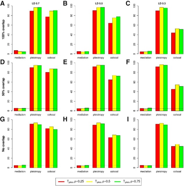
Type I error and power of when testing pleiotropy/colocalization against mediation using two variants at a locus. Type I error rate and power were evaluated at 0.05 significance level based on 1000 replicates. (A–C) Two traits have complete overlapped samples and the LD between two variants are r2=0.7, 0.5 and 0.3, respectively; (D–E) similar to (A–C) but with 50% overlapped samples; and (G–I) similar to (A–C) but with 0% overlapped samples (two-sample model). ρ represents trait correlation
Fig. 3.
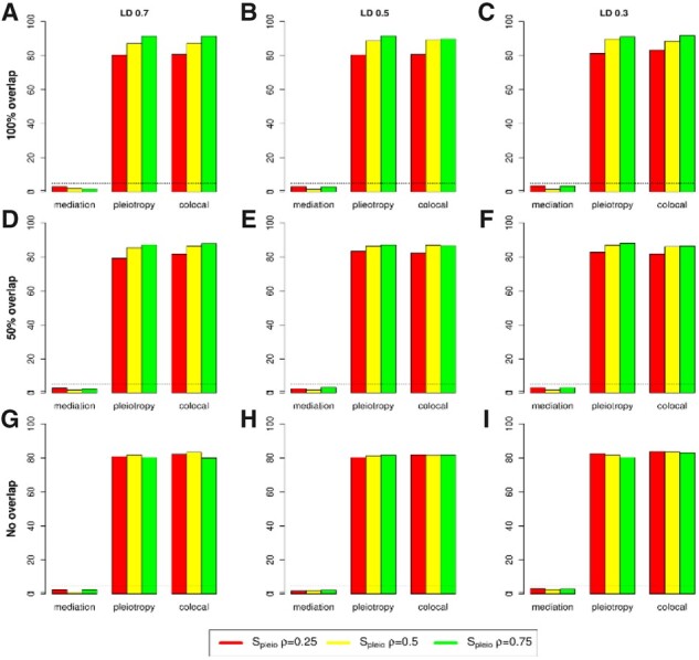
Type I error and power of when testing pleiotropy/colocalization against mediation using two variants at a locus. Type I error rate and power were evaluated at 0.05 significance level based on 1000 replications. (A–C) Two traits have complete overlapped samples and the LD between two variants are r2=0.7, 0.5 and 0.3, respectively; (D–E) similar to (A–C) but with 50% overlapped samples; and (G–I) similar to (A–C) but with 0% overlapped samples (two-sample model). ρ represents trait correlation
3.4. Data analysis
We applied IMRP, MR-PRESSO, IVW, MR-Egger, GSMR and MRmix to test for causal effect across a variety of exposures and health outcomes using publicly available summary statistics from large GWASs, which were analyzed by Qi and Chatterjee (2019). For each pair of traits, we selected genetic variants with exposure associated P-values <5×10⁻⁸. We ensured that both traits have the same effect allele and flipped the sign of the effect sizes for one trait when the effect allele was inconsistent. We pruned these variants using the software Plink (Purcell et al., 2007) based on 500 kb window size to identify independent variants as the IVs in MR analysis. For IMRP, the correlation was estimated between the standardized effect sizes of the exposure and the outcome after excluding the SNPs with the exposure associated P-values <0.01 using the GWAS summary statistics, as suggested in our previous studies (Park et al., 2016; Zhu et al., 2015). The number of IVs is presented in Table 2. Overall, the causal effects estimated by IMRP were similar to those estimated by MRmix and GSMR (Table 3). IMRP detected a substantial proportion of the IVs with significant pleiotropic effects (Table 3 and Supplementary Table S10). All the methods consistently detected significant causal roles of body mass index (BMI), systolic blood pressure (SBP), diastolic blood pressure (DBP) and LDL-C on the risk of coronary artery diseases (CAD). The estimated odds ratio (OR) for CAD ranged from 1.57 to 1.64 per SD unit increase in LDL. The IMRP, IVW, MR-PRESSO and GSMR analyses detected protective effect of high-density lipoprotein cholesterol (HDL-C) on CAD while MRmix and MR-Egger did not. IMRP estimated OR for CAD was 0.93 per SD unit increase in HDL, and GSMR had the largest and most significant estimated OR. When we pruned the IVs using Plink based on 1 Mb window size, the MRmix estimate became significant while MR-Egger did not, and the GSMR estimated OR was 0.65, the smallest and most significant one (Table 3). In comparison, the IMRP estimated OR was stable. Since colocalization may bias the causal effect estimate, we performed Spleio analysis for all the 87 IVs and identified 48 of them showing colocalization or pleiotropy evidence (Table 2 and Supplementary Table S11). After excluding the IVs with colocalization or pleiotropy evidence, the OR estimates were similar for IMRP, IVW, MR-PRESSO and GSMR. However, MRmix had smallest OR estimate but with large standard error, possibly due to small number of IVs (48). All the methods had similar OR estimate of triglycerides (TGs) on CAD.
Table 3.
Causal effect estimates by IMRP, IVW, MR-Egger and MRmix using the real GWAS data
| IMRP | IVW | MR-Egger | MRMix | MR-PRESSO | GSMR | |||||||||||||
|---|---|---|---|---|---|---|---|---|---|---|---|---|---|---|---|---|---|---|
| Outcome | Exposure | NIVs |
(se) |
P | Global test | NPV |
(se) |
P |
Intercept
P-value |
(se) |
P |
(se) |
P |
(se) |
P |
(se) |
P | |
| CAD | BMI | 1493 |
0.43
(0.02) |
1.28×10−92 | 2.99×10−38 | 11 |
0.39
(0.03) |
4.33×10−57 | 1.53×10⁻³ |
0.65
(0.09) |
5.24×10⁻¹⁴ |
0.46
(0.04) |
2.23×10⁻³⁰ | — | — | — |
0.41
(0.02) |
6.02×10−89 |
| SBP | 231 |
0.62
(0.04) |
9.39×10−50 | 5.30×10−88 | 14 |
0.56
(0.07) |
7.77×10⁻¹³ | 6.9×10⁻¹ |
0.69
(0.33) |
0.039 |
0.69
(0.09) |
4.08×10⁻¹⁶ |
0.61
(0.05) |
5.83×10⁻²³ | 12 |
0.66
(0.04) |
9.05×10−64 | |
| DBP | 258 |
0.49
(0.04) |
2.41×10⁻³⁴ | 6.01×10−76 | 15 |
0.53
(0.07) |
2.0×10⁻¹⁴ | 2.22×10⁻¹ |
0.89
(0.30) |
3.62×10⁻³ |
0.55
(0.10) |
1.51×10⁻⁸ |
0.54
(0.05) |
7.47×10⁻²¹ | 12 |
0.60
(0.04) |
2.58×10−59 | |
| HDLa | 143 |
−0.08
(0.03) |
5.19 10−3 | 1.39×10−65 | 10 |
−0.16
(0.05) |
5.1×10⁻⁴ | 2.0×10⁻³ |
0.06
(0.08) |
0.471 |
−0.04
(0.09) |
0.642 |
−0.18
(0.04) |
6.11×10⁻⁶ | 11 |
−0.10
(0.02) |
2.56×10⁻⁵ | |
| HDLb | 87 |
−0.11
(0.04) |
3.90×10⁻³ | 6.29×10−51 | 7 |
−0.25
(0.06) |
1.48×10⁻⁴ | 2.93×10⁻³ |
0.07
(0.12) |
0.629 |
−0.49
(0.11) |
1.50×10⁻⁵ |
−0.26
(0.05) |
1.48×10⁻⁶ | 9 |
−0.43
(0.04) |
8.63×10⁻²⁹ | |
| HDLc (Spleio) | 40 |
−0.16
(0.07) |
1.72×10⁻² | 1.16×10⁻⁷ | 1 |
−0.26
(0.09) |
8.74×10⁻³ | 0.104 |
0.25
(0.32) |
0.431 |
−0.37
(0.98) |
0.706 |
−0.21
(0.08) |
1.11×10⁻² | 1 |
−0.21
(0.06) |
2.38×10⁻⁴ | |
| LDL | 168 |
0.49
(0.02) |
5.62×10−105 | 2.72×10−49 | 7 |
0.46
(0.04) |
4.93×10−38 | 7.5×10⁻¹ |
0.48
(0.07) |
1.15×10⁻¹⁰ |
0.51
(0.04) |
7.10×10−44 |
0.45
(0.03) |
5.19×10−38 | 6 |
0.45
(0.02) |
2.70×10−118 | |
| TG | 120 |
0.24
(0.03) |
1.09×10⁻¹⁷ | 3.13×10⁻²² | 3 |
0.22
(0.04) |
3.64×10⁻⁸ | 2.08×10⁻¹ |
0.14
(0.07) |
0.054 |
0.65
(0.11) |
6.71×10⁻⁹ |
0.23
(0.04) |
1.69×10⁻⁹ | 3 |
0.23
(0.02) |
1.51×10⁻²³ | |
| BC | BMI | 1493 |
−0.07
(0.02) |
2.18×10⁻³ | 1.17×10−59 | 8 |
−0.13
(0.03) |
9.76×10⁻⁶ | 2.87×10⁻⁵ |
−0.52
(0.10) |
1.23×10⁻⁷ |
−0.14
(0.05) |
2.16×10⁻³ | — | — | — |
−0.17
(0.02) |
4.21×10⁻¹⁴ |
| Height | 5411 |
0.01
(0.01) |
0.185 | 3.28×10−136 | 20 |
0.03
(0.01) |
1.24×10⁻³ | 5.98×10⁻¹ |
0.04
(0.03 ) |
0.124 |
0.0
(0.03) |
1.0 | — | — | — |
0.0
(0.01) |
0.699 | |
| HDL | 143 |
−0.10
(0.03) |
1.94×10⁻⁴ | 8.19×10⁻⁷ | 1 |
−0.09
(0.03) |
3.9×10⁻³ | 2.19×10⁻³ |
−0.06
(0.06) |
0.299 |
−0.06
(0.03) |
0.053 |
−0.08
(0.03) |
3.41×10⁻³ | 1 |
−0.07
(0.02) |
2.38×10⁻³ | |
| LDL | 168 |
0.03
(0.02) |
0.177 | 3.37×10⁻⁹ | 1 |
−0.05
(0.03) |
0.043 | 1.08×10⁻² |
0.05
(0.05) |
0.275 |
0.49
(0.12) |
7.18×10⁻⁵ |
0.05
(0.03) |
0.08 | 1 |
0.03
(0.02) |
0.079 | |
| TG | 120 |
0.0
(0.03) |
0.896 | 6.64×10⁻⁸ | 0 |
0.01
(0.03) |
0.679 | 2.53×10⁻¹ |
0.07
(0.06) |
0.233 |
−0.02
(0.05) |
0.691 |
0.01
(0.03) |
0.750 | 0 |
0.02
(0.02) |
0.416 | |
| AM | 344 |
−0.04
(0.03) |
0.265 | 1.75×10⁻²⁰ | 4 |
−0.01
(0.04) |
0.727 | 9.30×10⁻¹ |
0.0
(0.14) |
0.984 |
0.09
(0.09) |
0.310 |
0.03
(0.04) |
0.388 | 3 |
−0.01
(0.03) |
0.772 | |
| MDD | BMI | 1046 |
0.20
(0.02) |
1.16×10⁻¹⁹ | 2.33×10−48 | 3 |
0.17
(0.03) |
7.56×10⁻¹⁰ | 3.80×10⁻¹ |
0.09
(0.09) |
0.357 |
0.34
(0.10) |
3.42×10⁻⁴ | — | — | — |
0.22
(0.02) |
5.49×10⁻²⁷ |
| EA | 380 |
−0.25
(0.02) |
7.77×10⁻²⁰ | 4.35×10⁻²³ | 3 |
−0.20
(0.03) |
1.03×10⁻⁸ | 6.87×10⁻¹ |
−0.27
(0.18) |
0.1259 |
−0.34
(0.17) |
0.04 |
−0.20
(0.03) |
2.17×10⁻⁹ | 4 |
−0.20
(0.03) |
5.25×10⁻¹⁵ | |
Note: CAD, coronary artery disease; BC, breast cancer; MDD, major depressive disorder; AM, age at menarche; EA, educational attainment; LDL, low-density lipoprotein; HDL, high-density lipoprotein; TG, triglyceride; DBP, diastolic blood pressure; SBP, systolic blood pressure; NIV, the number of IVs pruned based on 500 kb window sizes in the GWAS study associated with exposure; NPV, the number of IVs are significant in pleiotropy test after correcting for multiple comparisons; HDLa, number of IVs pruned based on 500 kb window size; HDLb, number of IVs pruned based on 1 Mb window size; HDLc, pleiotropy was tested by Spleio; ‘—’, MR_PRESSO was failed to run because of large number of IVs when the Null distribution was calculated based on 10 000 simulations.
Bolded P-values suggest significant causal effects.
All the methods detected a significant protective causal effect of BMI on the risk of breast cancer (BC) with estimated OR ranged from 0.60 to 0.93, except that the MR-Egger estimate was not significant. MR-PRESSO failed to perform MR analysis for BMI and height because of the large numbers of IVs. The IMRP, IVW, MR-PRESSO and GSMR analyses detected inverse causal effect of HDL-C on the risk of BC with OR ranged from 0.90 to 0.94 per SD unit increase in HDL-C, while both MRmix and IVW detected significant causal relationship of LDL-C and BC but in opposite causal directions. IMRP, MRmix, MR-Egger, MR-PRESSO and GSMR did not detect a causal relationship between height, TG and age at menarche with BC, and significant causal evidence of height, LDL-C on BC was suggested by IVW analysis. Interestingly, MRmix also suggested significant causal relationship of LDL-C on BC. All methods except for MR-Egger detected a significant protective causal effect of BMI and educational attendance (EA) on the risk of major depressive disorder (MDD). The estimated OR ranged from 1.18 to 1.4 for BMI and 0.71 to 0.84 for EA. The MR-Egger analysis did not detect causal effect of BMI and EA on MDD. Finally, we found that IMRP was near three orders faster than MRMix in our HPC cluster at Case Western Reserve University. As demonstrated in the HDL-CAD analysis with 87 IVs, IMRP took 0.016 s in comparing with 15.394 s by MRMix, respectively.
4. Discussion
We presented a computationally efficient iterative approach (IMRP) for simultaneously performing MR analysis and detecting pleiotropic variants using GWAS summary statistics. IMRP iteratively searches for invalid IVs with pleiotropy effects on both exposure and outcome, and then estimates the causal effect of exposure on outcome after removing invalid IVs. IMRP is able to analyze summary statistics from either overlapped or non-overlapped data and is computationally efficient as it directly tests for pleiotropy from mediation without incurring simulations. A recently developed MR analysis method, MR-PRESSO, also detects pleiotropy and estimates the causality after removing the invalid IVs. MR-PRESSO constructs a pleiotropic test based on time-consuming simulations. To compare the performance of IMRP and MR-PRESSO, we performed simulations under a variety of causal models by allowing different genetic contributions to exposure and outcome. In most situations, IMRP had better power to detect IVs with pleiotropic effect when InSIDE was valid (Table 1 and Supplementary Tables S1–S4) and hence was less biased in estimating causal effect than MR-PRESSO (Table 2 and Supplementary Tables S5–S8). When InSIDE was invalid, MR-PRESSO detected more pleiotropic variants but also increased false positive rates. In practice, we observed that IMRP and MR-PRESSO detected similar number of pleiotropic variants, although slightly more pleiotropic variants for IMRP than MR-PRESSO were observed in some cases, which is consistent with the simulations. IMRP was three order faster than MR-PRESSO or MRMix. The computational requirement on MR-PRESSO will deteriorate rapidly when the number of IVs increases, as we observed in the real data BMI and height analysis, but it has no effect on IMRP. We observed that the IMRP analysis usually needed <10 iterations. IMRP provides the global test statistic that follows a χ2 distribution with degrees of freedom equaling to the number of IVs reduced by 1. is able to assess whether there are remaining pleiotropic variants after excluding variants with significant pleiotropic effects. If so, further exclusion of potential invalid IVs can be applied, as demonstrated in the real data analysis, where we detected many IVs with pleiotropic effects (Supplementary Table S10) after correcting for the number of IVs in each of exposure-outcome analysis. However, the global test statistic was often significant even after excluding variants with significant pleiotropic evidence, suggesting that a large number of pleiotropic variants still exist. The global test statistic was no long significant when we further excluded all IVs with pleiotropic test P-value <0.05 in all the real data analysis.
The pleiotropy test for single variant is extended to for multiple variants at a locus. Our simulations demonstrated that is more powerful for detecting colocalization than (Figs 2 and 3). In HDL-C and CAD analysis, we observed many variants with colocalization or pleiotropic evidence (Supplementary Table S11). The is able to detect pleiotropy effects contributed by multiple causal variants, providing that the causal effect is known. In MR analysis, when a genetic variant in test only shows nominal significance in pleiotropic test, we can further apply and multiple variants at the same locus to verify if the variant has evidence of pleiotropy or colocalization, as we did in real data analysis. Thus, the statistic should be applied with MR analysis together for detecting colocalization.
When ZEMPA assumption is not satisfied, IMRP may remove the valid IVs in its iterations, resulting in bias or loss of power. IMRP shares similarity with GSMR but also has substantial differences. IMRP uses all independent significant variants associated with exposure in the MR analysis and automatically determines which variants to be removed in an iterative way. In comparison, GSMR uses causal estimates of top variants in the pleiotropic test. In particular, GSMR chooses the SNP that shows the strongest association with the exposure in the third quantile of the distribution. This selection is subjective, as suggested by Hemani et al. (2018). In our simulations, we observed that the performance of GSMR was similar to MR-PRESSO and IVW. When the number of IVs was <50 and 50% or 90% IVs were pleiotropic variants, GSMR often failed to estimate the causal effects. IMRP uses the MR-Egger estimate as its initial estimate, followed by IVW, to take the advantages of MR-Egger, which is less biased when pleiotropy is present or InSIDE assumption is not valid (Bowden et al., 2015), and IVW, which has less uncertainty. In theory, MR-Egger estimate is not consistent when InSIDE assumption is violated. However, our simulations demonstrated that the causal effect estimate of MR-Egger is less biased but with larger standard error than that of IVW when the InSIDE assumption is violated (Table 2 and Supplementary Tables S6 and S8). This is consistent with what observed in the original MR-Egger study (Bowden et al., 2015). When InSIDE assumption is violated, a genetic IV can affect both exposure and outcome through a confounder, which is similar to a pleiotropic variant. The difference is that the effects on the exposure and outcome can be independent for a pleiotropic variant but dependent for a variant violating InSIDE. Thus, the intercept of the MR-Egger regression will still capture some of the violation and therefore reduces the bias in causal estimate, motivating us to take the MR-Egger estimate as the initial value. In comparison, when we took the initial estimate from IVW, the IMRP results were either similar or worse than when taking the initial estimate from MR-Egger (Supplementary Tables S5–S8). Therefore, we suggest taking the MR-Egger estimate as the initial causal estimate should be the first choice in the IMRP analysis in practice. In real data analysis, we also observed that taking MR-Egger estimate as the initial value will preserve power and reduce bias, which can be attributed to a large number of IVs and low proportion of pleiotropic IVs (<10%). When the number of IVs is large and the proportion of pleiotropic variants is low, regression noise can be reduced by dropping pleiotropic variants, while a good number of remained IVs can provide the adequate sample size in a weighted regression model to achieve satisfactory power for IMRP. This was demonstrated by our results, which showed that IMRP identified similar or more significant causal effects than IVW and MR-PRESSO (e.g. the causal effect estimates of BMI, SBP, DBP, LDL, TG on CAD and BMI and EA on MDD, Table 3). In some cases, GSMR had the most significant results, which may be at least partially due to potential bias. For example, no direct causal contribution of HDL to CAD was shown in clinical trials (Barter and Genest, 2019), but GSMR suggested a strong causal protective effect.
The proposed pleiotropic tests depend on the selection of IVs in estimating the causal effects. To reduce this selection bias, GSMR takes the SNP that shows the strongest association with the exposure in the third quantile of the distribution (Zhu et al., 2018). Currently IMRP takes all the SNPs significantly associated with the exposure in GWAS studies. It is possible that the most significant exposure associated variants will be more likely show pleiotropic evidence in the pleiotropic tests because of the ‘winner’s cures’. In this case, the procedure of GSMR can be easily adopted in the initial causal effect estimation in the IMRP analysis.
We compared IMRP with MRmix, IVW, MR-Egger, MR-PRESSO and GSMR analysis by reanalyzing the GWAS summary statistics data analyzed in Qi and Chatterjee (2019). MRmix (Qi and Chatterjee, 2019) is based on normal-mixture models and robust against potential model misspecification by relying on an estimating equation approach. IMRP has similar performance as MRmix in estimating causal effects although notable different results were also observed (Table 3). More recently, the horizontal pleiotropy score (HOPS) was developed for detecting horizontal pleiotropy (Jordan et al., 2019). However, the statistic of HOPS is not able to maintain type I error rate in testing horizontal pleiotropy, which warrants further investigation.
Many large-scale population studies reported an inverse relationship between HDL-C and CAD (Emerging Risk Factors Collaboration et al., 2009; Prospective Studies Collaboration et al., 2007). A MR analysis using 15 genetic variants as IVs did not suggest causal relationship between HDL-C and myocardial infarction (Voight et al., 2012), which was consistent with the evidence from a clinical trial study (Barter and Genest, 2019). The complex relationship between HDL-C and CAD leads to a debate over whether HDL-C is able to predict the risk of atherosclerotic cardiovascular disease (Barter and Genest, 2019). When using the 15 genetic variants from Voight et al. (2012), IMRP did not detect significant causal effect (P=0.58). However, when 143 IVs were used, IMRP, IVW, MR-PRESSO and GSMR detected a protective effect of HDL-C on the risk of CAD (OR 0.93 per SD unit increase in HDL) while MRmix and MR-Egger did not. Interestingly, reducing the number of IVs by pruning the IVs on 1 Mb window size, IMRP, IVW, MRmix, MR-PRESSO and GSMR all detected significant causal effect of HDL on CAD (Table 2) (OR 0.16–0.66 per SD unit increase in HDL), indicating the causal effect estimate is sensitive to the genetic IVs in MR analysis for MRmix. Applying Spleio identified additional IVs with either pleiotropy or colocalization evidence. After excluding these variants, IMRP, IVW, MR-PRESSO and GSMR still detected causal effect evidence but MRmix and MR-Egger did not. Overall, IMRP had less significant causal estimate of HDL-C on CAD than IVW, MR-PRESSO and GSMR, suggesting IMRP is less biased than IVW, MR-PRESSO and GSMR. Our results, together with others (Holmes et al., 2015; Voight et al., 2012), may suggest that the causal role for HDL-C on CVD risk is weak if it exists. IMRP identified risk effect of TGs (OR 1.27) on CAD while MRmix did not. Population-based epidemiology studies consistently suggested that TG level predicts cardiovascular risk (Harchaoui et al., 2009; Singh and Singh, 2016). The recent large clinical trial REDUCE-IT showed that reducing TG levels decreased cardiovascular death (Bhatt et al., 2019), which was consistent with our IMRP analysis. Since HDL-C and TG are negatively correlated and genetic variants contribute to both traits, conditional on HDL-C, the genetic variants can still affect CAD by the mediation of TG. Therefore, the causal effect estimation of the MR analysis by excluding pleiotropy variants for HDL-C and CAD can still be biased (Zhu, 2020).
A consistent negative causal effect of BMI on the risk of BC was observed by IMRP and other methods (Table 2). The inferred negative causal relationship between BMI and BC seems inconsistent with positive association observed in epidemiologic studies. Previous MR analysis using fewer IVs revealed the inverse causal relationship between BMI and BC (Guo et al., 2016; Qi and Chatterjee, 2019), although the effect size of IMRP was attenuated (OR 0.93). IMRP, IVW, MR-PRESSO and GSMR identified a significant inverse causal effect of HDL-C on the risk of BC while MRmix and IVW detected an inverse causal relationship of LDL-C on BC, which are consistent with the direct associations observed in epidemiologic studies (Cedo et al., 2019). We did not observe the causal relationship between age at menarche and BC suggested by the previous MRmix analysis (Qi and Chatterjee, 2019), potentially due to different number of IVs used. IMRP detected a significant causal risk effect of BMI but a protective effect of EA on MDD, so did MRmix, IVW and GSMR. However, MR-PRESSO was not able to handle the large numbers of IVs for BMI and height.
Following CP association approaches that focus on detecting overall association evidence of a variant with multiple traits, IMRP is able to differentiate whether CP association (Zhu et al., 2015) is caused by mediation or pleiotropic effect, which provides a better understanding of causal relationship between two correlated traits. Recent advances in estimating shared genetic correlations (Bulik-Sullivan et al., 2015; Lee et al., 2012; Loh et al., 2015; Visscher et al., 2014) provide insights into the genetic architecture among correlated traits. However, these methods provide limited information about how individual variants affect multiple traits, a gap that can be filled by the IMRP analysis.
IMRP identified many pleiotropic variants among all the pairs of exposure and outcome in the real data analysis (Table 2 and Supplementary Table S10), consistent with a recent observation that many disease-associated variants identified from GWASs have effects on multiple traits (Gratten and Visscher, 2016; Watanabe et al., 2019). It is then important to identify the IVs with pleiotropic effects in performing MR analysis.
In conclusion, IMRP is a novel efficient tool for performing MR analysis and identifying pleiotropic variants using summary statistics from GWAS. In addition, IMRP is able to identify colocalization for multiple variants in a locus. Through both simulations and real data applications, we demonstrated that IMRP has better trade-off between bias and variance than alternatives and is a robust and powerful tool for understanding causal relationship among correlated traits using genetic instruments.
Supplementary Material
Acknowledgements
We thank Noah Lorincz-Comi for helping to upload the IMRP software to github.
Authors’ contributions
X.Z. conceived and designed the study. X.Z. and X.L. performed simulations. X.Z. performed real data analysis. X.Z. and X.L. drafted the manuscript. All co-authors substantively revised the manuscript.
Funding
This work was supported by grants HG003054, HG011052 (to X.Z.) from the National Human Genome Research Institute, R21 CA202529 (to T.W.) and by grants AG057557-01, AG061388-01 and AG062272-01 (to R.X.) from the National Institute on Aging.
Conflict of Interest
There is no conflict of interest.
Data availability
The GWAS summary statistics used in this study are publicly available at the following URLs. GIANT Consortium (BMI and height) summary statistics, http://portals.broadinstitute.org/collaboration/giant/index.php/GIANT_consortium_data_files; Global Lipids Genetics Consortium (cholesterol traits), http://csg.sph.umich.edu/abecasis/public/lipids2013/; ReproGen Consortium (age at menarche), http://www.reprogen.org/data_download.html; Social Science Genetic Association Consortium (SSGAC), https://www.thessgac.org/data; CARDIoGRAMplusC4D Consortium (coronary artery disease), http://www.cardiogramplusc4d.org/data-downloads/; Breast Cancer Association Consortium (BCAC) summary statistics, http://bcac.ccge.medschl. cam.ac.uk/bcacdata/oncoarray/gwas-icogs-and-oncoarray-summary-results/; Psychiatric Genomics Consortium (PGC), https://www.med.unc.edu/pgc/results-and-downloads/.
Contributor Information
Xiaofeng Zhu, Department of Population and Quantitative Health Sciences, School of Medicine, Case Western Reserve University, Cleveland, OH 44106, USA.
Xiaoyin Li, Department of Population and Quantitative Health Sciences, School of Medicine, Case Western Reserve University, Cleveland, OH 44106, USA.
Rong Xu, Center for Artificial Intelligence in Drug Discovery, School of Medicine, Case Western Reserve University, Cleveland, OH 44106, USA.
Tao Wang, Division of Biostatistics, Department of Epidemiology and Population Health, Albert Einstein College of Medicine of Yeshiva University, Bronx, NY 10461, USA; Division of Epidemiology, Department of Epidemiology and Population Health, Albert Einstein College of Medicine of Yeshiva University, Bronx, NY 10461, USA.
References
- Andreassen O.A. et al. ; Psychiatric Genomics Consortium Schizophrenia Working Group. (2013) Improved detection of common variants associated with schizophrenia by leveraging pleiotropy with cardiovascular-disease risk factors. Am. J. Hum. Genet., 92, 197–209. [DOI] [PMC free article] [PubMed] [Google Scholar]
- Barbeira A.N. et al. ; GTEx Consortium. (2018) Exploring the phenotypic consequences of tissue specific gene expression variation inferred from GWAS summary statistics. Nat. Commun., 9, 1825. [DOI] [PMC free article] [PubMed] [Google Scholar]
- Barter P., Genest J. (2019) HDL cholesterol and ASCVD risk stratification: a debate. Atherosclerosis, 283, 7–12. [DOI] [PubMed] [Google Scholar]
- Bhatt D.L. et al. (2019) Cardiovascular risk reduction with icosapent ethyl for hypertriglyceridemia. N. Engl. J. Med., 380, 11–22. [DOI] [PubMed] [Google Scholar]
- Borenstein M. et al. (2009) Generality of the basic inverse-variance method. In: Introduction to Meta-Analysis. Wiley, Chichester, UK, pp. 311–319. [Google Scholar]
- Bowden J. et al. (2015) Mendelian randomization with invalid instruments: effect estimation and bias detection through Egger regression. Int. J. Epidemiol., 44, 512–525. [DOI] [PMC free article] [PubMed] [Google Scholar]
- Bulik-Sullivan B. et al. ; ReproGen Consortium. (2015) An atlas of genetic correlations across human diseases and traits. Nat. Genet., 47, 1236–1241. +. [DOI] [PMC free article] [PubMed] [Google Scholar]
- Bulik-Sullivan B.K. et al. ; Schizophrenia Working Group of the Psychiatric Genomics Consortium. (2015) LD Score regression distinguishes confounding from polygenicity in genome-wide association studies. Nat. Genet., 47, 291–295. [DOI] [PMC free article] [PubMed] [Google Scholar]
- Burgess S. et al. (2017) Sensitivity analyses for robust causal inference from Mendelian randomization analyses with multiple genetic variants. Epidemiology, 28, 30–42. [DOI] [PMC free article] [PubMed] [Google Scholar]
- Cedo L. et al. (2019) HDL and LDL: potential new players in breast cancer development. J. Clin. Med., 8, 853. [DOI] [PMC free article] [PubMed] [Google Scholar]
- Cortes A. et al. (2020) Identifying cross-disease components of genetic risk across hospital data in the UK Biobank. Nat. Genet., 52, 126–134. [DOI] [PMC free article] [PubMed] [Google Scholar]
- Cotsapas C. et al. ; on behalf of the FOCiS Network of Consortia. (2011) Pervasive sharing of genetic effects in autoimmune disease. PLoS Genet., 7, e1002254. [DOI] [PMC free article] [PubMed] [Google Scholar]
- Davey Smith G. (2015) Mendelian randomization: a premature burial? bioRxiv, 021386. [Google Scholar]
- Davey Smith G., Hemani G. (2014) Mendelian randomization: genetic anchors for causal inference in epidemiological studies. Hum. Mol. Genet., 23, R89–R98. [DOI] [PMC free article] [PubMed] [Google Scholar]
- Emerging Risk Factors Collaboration et al. (2009) Major lipids, apolipoproteins, and risk of vascular disease. JAMA, 302, 1993–2000. [DOI] [PMC free article] [PubMed] [Google Scholar]
- Evans D.M., Davey Smith G. (2015) Mendelian randomization: new applications in the coming age of hypothesis-free causality. Annu. Rev. Genomics Hum. Genet., 16, 327–350. [DOI] [PubMed] [Google Scholar]
- Franceschini N. et al. (2013) Genome-wide association analysis of blood-pressure traits in African-ancestry individuals reveals common associated genes in African and non-African populations. Am. J. Hum. Genet., 93, 545–554. [DOI] [PMC free article] [PubMed] [Google Scholar]
- Giambartolomei C. et al. (2014) Bayesian test for colocalisation between pairs of genetic association studies using summary statistics. PLoS Genet., 10, e1004383. [DOI] [PMC free article] [PubMed] [Google Scholar]
- Gratten J., Visscher P.M. (2016) Genetic pleiotropy in complex traits and diseases: implications for genomic medicine. Genome Med., 8, 78. [DOI] [PMC free article] [PubMed] [Google Scholar]
- Guo Y. et al. (2016) Genetically predicted body mass index and breast cancer risk: Mendelian randomization analyses of data from 145,000 women of European descent. PLoS Med., 13, e1002105. [DOI] [PMC free article] [PubMed] [Google Scholar]
- Harchaoui K.E. et al. (2009) Triglycerides and cardiovascular risk. Curr. Cardiol. Rev., 5, 216–222. [DOI] [PMC free article] [PubMed] [Google Scholar]
- Hemani G. et al. (2018) Evaluating the potential role of pleiotropy in Mendelian randomization studies. Hum. Mol. Genet., 27, R195–R208. [DOI] [PMC free article] [PubMed] [Google Scholar]
- Holmes M.V. et al. ; on behalf of the UCLEB consortium. (2015) Mendelian randomization of blood lipids for coronary heart disease. Eur. Heart J., 36, 539–550. [DOI] [PMC free article] [PubMed] [Google Scholar]
- Hormozdiari F. et al. (2016) Colocalization of GWAS and eQTL signals detects target genes. Am. J. Hum. Genet., 99, 1245–1260. [DOI] [PMC free article] [PubMed] [Google Scholar]
- Jordan D.M. et al. (2019) HOPS: a quantitative score reveals pervasive horizontal pleiotropy in human genetic variation is driven by extreme polygenicity of human traits and diseases. Genome Biol., 20, 222. [DOI] [PMC free article] [PubMed] [Google Scholar]
- Lee S.H. et al. (2012) Estimation of pleiotropy between complex diseases using single-nucleotide polymorphism-derived genomic relationships and restricted maximum likelihood. Bioinformatics, 28, 2540–2542. [DOI] [PMC free article] [PubMed] [Google Scholar]
- Liang J. et al. (2017) Single-trait and multi-trait genome-wide association analyses identify novel loci for blood pressure in African-ancestry populations. PLoS Genet., 13, e1006728. [DOI] [PMC free article] [PubMed] [Google Scholar]
- Loh P.R. et al. ; Schizophrenia Working Group of the Psychiatric Genomics Consortium. (2015) Contrasting genetic architectures of schizophrenia and other complex diseases using fast variance-components analysis. Nat. Genet., 47, 1385–1392. [DOI] [PMC free article] [PubMed] [Google Scholar]
- Park H. et al. (2016) Multivariate analysis of anthropometric traits using summary statistics of genome-wide association studies from GIANT consortium. PLoS One, 11, e0163912. [DOI] [PMC free article] [PubMed] [Google Scholar]
- Pickrell J. (2015) Fulfilling the promise of Mendelian randomization. bioRxiv, 018150. [Google Scholar]
- Pomerantz M.M. et al. (2009) The 8q24 cancer risk variant rs6983267 shows long-range interaction with MYC in colorectal cancer. Nat. Genet., 41, 882–884. [DOI] [PMC free article] [PubMed] [Google Scholar]
- Prospective Studies Collaboration et al. (2007) Blood cholesterol and vascular mortality by age, sex, and blood pressure: a meta-analysis of individual data from 61 prospective studies with 55,000 vascular deaths. Lancet, 370, 1829–1839. [DOI] [PubMed] [Google Scholar]
- Purcell S. et al. (2007) PLINK: a tool set for whole-genome association and population-based linkage analyses. Am. J. Hum. Genet., 81, 559–575. [DOI] [PMC free article] [PubMed] [Google Scholar]
- Qi G., Chatterjee N. (2019) Mendelian randomization analysis using mixture models for robust and efficient estimation of causal effects. Nat. Commun., 10, 1941. [DOI] [PMC free article] [PubMed] [Google Scholar]
- Singh A.K., Singh R. (2016) Triglyceride and cardiovascular risk: a critical appraisal. Indian J. Endocrinol. Metab., 20, 418–428. [DOI] [PMC free article] [PubMed] [Google Scholar]
- Solovieff N. et al. (2013) Pleiotropy in complex traits: challenges and strategies. Nat. Rev. Genet., 14, 483–495. [DOI] [PMC free article] [PubMed] [Google Scholar]
- Turley P. et al. ; 23andMe Research Team. (2018) Multi-trait analysis of genome-wide association summary statistics using MTAG. Nat. Genet., 50, 229–237. [DOI] [PMC free article] [PubMed] [Google Scholar]
- Verbanck M. et al. (2018) Detection of widespread horizontal pleiotropy in causal relationships inferred from Mendelian randomization between complex traits and diseases. Nat. Genet., 50, 693–698. [DOI] [PMC free article] [PubMed] [Google Scholar]
- Visscher P.M. et al. (2014) Statistical power to detect genetic (co)variance of complex traits using SNP data in unrelated samples. PLoS Genet., 10, e1004269. [DOI] [PMC free article] [PubMed] [Google Scholar]
- Voight B.F. et al. (2012) Plasma HDL cholesterol and risk of myocardial infarction: a Mendelian randomisation study. Lancet, 380, 572–580. [DOI] [PMC free article] [PubMed] [Google Scholar]
- Wagner G.P., Zhang J. (2011) The pleiotropic structure of the genotype-phenotype map: the evolvability of complex organisms. Nat. Rev. Genet., 12, 204–213. [DOI] [PubMed] [Google Scholar]
- Wasserman N.F. et al. (2010) An 8q24 gene desert variant associated with prostate cancer risk confers differential in vivo activity to a MYC enhancer. Genome Res., 20, 1191–1197. [DOI] [PMC free article] [PubMed] [Google Scholar]
- Watanabe K. et al. (2019) A global overview of pleiotropy and genetic architecture in complex traits. Nat.Genet., 51, 1339–1348 [DOI] [PubMed] [Google Scholar]
- Wen X. et al. (2017) Integrating molecular QTL data into genome-wide genetic association analysis: probabilistic assessment of enrichment and colocalization. PLoS Genet., 13, e1006646. [DOI] [PMC free article] [PubMed] [Google Scholar]
- Yan T. et al. ; The Alzheimer Disease Neuroimaging Initiative. (2020) FAM222A encodes a protein which accumulates in plaques in Alzheimer's disease. Nat. Commun., 11, 411. [DOI] [PMC free article] [PubMed] [Google Scholar]
- Zhu X. (2020) Mendelian randomization and pleiotropy analysis. Quant. Biol., 10.1007/s40484-020-0216-3. [DOI] [PMC free article] [PubMed] [Google Scholar]
- Zhu X. et al. (2015) Meta-analysis of correlated traits via summary statistics from GWASs with an application in hypertension. Am. J. Hum. Genet., 96, 21–36. [DOI] [PMC free article] [PubMed] [Google Scholar]
- Zhu Z. et al. (2018) Causal associations between risk factors and common diseases inferred from GWAS summary data. Nat. Commun., 9, 224. [DOI] [PMC free article] [PubMed] [Google Scholar]
Associated Data
This section collects any data citations, data availability statements, or supplementary materials included in this article.
Supplementary Materials
Data Availability Statement
The GWAS summary statistics used in this study are publicly available at the following URLs. GIANT Consortium (BMI and height) summary statistics, http://portals.broadinstitute.org/collaboration/giant/index.php/GIANT_consortium_data_files; Global Lipids Genetics Consortium (cholesterol traits), http://csg.sph.umich.edu/abecasis/public/lipids2013/; ReproGen Consortium (age at menarche), http://www.reprogen.org/data_download.html; Social Science Genetic Association Consortium (SSGAC), https://www.thessgac.org/data; CARDIoGRAMplusC4D Consortium (coronary artery disease), http://www.cardiogramplusc4d.org/data-downloads/; Breast Cancer Association Consortium (BCAC) summary statistics, http://bcac.ccge.medschl. cam.ac.uk/bcacdata/oncoarray/gwas-icogs-and-oncoarray-summary-results/; Psychiatric Genomics Consortium (PGC), https://www.med.unc.edu/pgc/results-and-downloads/.