Causal Inference in high dimensions: A marriage between Bayesian modeling and good frequentist properties

Summary:

We introduce a framework for estimating causal effects of binary and continuous treatments in high dimensions. We show how posterior distributions of treatment and outcome models can be used together with doubly robust estimators. We propose an approach to uncertainty quantification for the doubly robust estimator which utilizes posterior distributions of model parameters and (1) results in good frequentist properties in small samples, (2) is based on a single MCMC, and (3) improves over frequentist measures of uncertainty which rely on asymptotic properties. We consider a flexible framework for modeling the treatment and outcome processes within the Bayesian paradigm that reduces model dependence, accommodates nonlinearity, and achieves dimension reduction of the covariate space. We illustrate the ability of the proposed approach to flexibly estimate causal effects in high dimensions and appropriately quantify uncertainty. We show that our proposed variance estimation strategy is consistent when both models are correctly specified, and we see empirically that it performs well in finite samples and under model misspecification. Finally, we estimate the effect of continuous environmental exposures on cholesterol and triglyceride levels.

1. Introduction

There has been a rapid growth in the interest of estimating the causal effect of a treatment (T) on an outcome (Y) when the dimension of the covariate space (X) is large relative to the sample size. In high-dimensions, some form of dimension reduction or variable selection is required, and traditional approaches to reducing the dimension of the parameter space can lead to biased estimators with nonregular asymptotic behavior. Recent work has focused on tailoring these approaches to the specific problem of estimating treatment effects in high dimensions. Tan (2020b) extended inverse propensity weighted estimators to this setting, and estimated the propensity scores with a combination of regularization and calibration to improve inference on treatment effects. However, most approaches utilize both the treatment and outcome to reduce the dimension of the parameter space to reduce confounding bias. Belloni et al. (2014) suggested using a post-selection estimator based on the union of variables selected from a first-stage treatment and outcome model, and showed that the resulting inference on treatment effects is uniformly valid. Athey et al. (2018) combine outcome regression models with weights that balance any remaining differences in covariates between treated and control units. Other approaches have focused on one of either the treatment or outcome model, but allowed the amount of shrinkage or regularization to depend on the parameters of the other model in a way that improves finite sample performance (Antonelli et al., 2019; Shortreed and Ertefaie, 2017; Hahn et al., 2018). Relatedly, Ertefaie et al. (2018) derived a penalization-based estimator that incorporates information from both the treatment and outcome to identify confounders, and estimates treatment effects conditional on this chosen set.

While most of the previous approaches utilized both a treatment and outcome model, none are doubly robust in the sense that only one of the two models needs to be correctly specified for consistent estimation of treatment effects. Doubly robust estimators have been widely used in the causal inference literature (Bang and Robins, 2005), as they allow for increased robustness to model misspecification and allow for data-adaptive estimation of the treatment and outcome model. See Daniel (2014) for a nice overview of doubly robust estimators and their properties. These estimators have been extended to high-dimensional settings (Farrell, 2015; Chernozhukov et al., 2018), but inference for these estimators is not doubly robust: While they are consistent when only one of the two models is correctly specified, corresponding confidence intervals rely on both models being correctly specified to obtain valid inference. Other approaches that provide doubly robust point estimators but not confidence intervals include doubly robust matching estimators (Antonelli et al., 2016) or targeted maximum likelihood estimators (Van Der Laan and Rubin, 2006) combined with high-dimensional models. To address this gap in the literature, recent work has looked to construct doubly robust estimators that simultaneously admit doubly robust inference. Avagyan and Vansteelandt (2020) construct estimates of treatment and outcome model parameters using penalized estimating equations to produce so-called bias-reduced doubly robust estimators, which in turn lead to valid inference even when one model is misspecified, though this approach does not extend to cases where the parameter space is larger than the sample size. Dukes et al. (2020) construct tests for the null hypothesis of no treatment effect that are valid even when one model is misspecified. They assume strong conditions on the sparsity of the treatment and outcome models, but show that these conditions can be weakened when both models are correctly specified. Ning et al. (2020) achieve doubly robust inference through covariate balancing propensity scores that target balance of variables that are associated with the outcome, while Tan (2020a) achieve doubly robust inference through calibrated propensity scores and weighted penalized outcome models. Both of these approaches rely on strong sparsity assumptions, as well as linearity assumptions for the outcome model. Despite providing doubly robust confidence intervals, inference for all of these approaches is based on asymptotic arguments that may not perform well in finite samples.

In this paper, we propose a doubly robust estimator that is based on Bayesian models for the treatment and outcome model, and an approach to inference on treatment effects with improved finite sample performance. Our inferential approach uses the posterior distribution of both models, and it does not rely on asymptotic approximations or on correct model specification. We show theoretically that our proposed variance estimator is consistent as long as both models are correctly specified, and that it is generally conservative in finite samples or when one or both models are misspecified. This is related to existing work that aims to improve inference for doubly robust estimators under model misspecification, though our work differs in that it explicitly focuses on finite sample variance estimation. Importantly, our results do not rely on linearity of the treatment or outcome model, and very complex models such as tree-based models or Gaussian process specifications can be used. We show that the proposed approach is directly applicable to high-dimensional settings with continuous treatments, a scenario that has been overlooked in the literature. We show empirically that the proposed procedure leads to improved performance, in particular with respect to inference in finite samples, when existing approaches that rely on asymptotics do not perform well.

2. Notation, estimands, and identifying assumptions

Let T and Y be the treatment and outcome of interest, respectively, while X is a p–dimensional vector of potential confounders. We observe an i.i.d sample D_i = (X_i, T_i, Y_i) for i = 1 … n, and denote D = (D₁, D₂, …, D_n). We work under the high-dimensional situation where the number of covariates exceeds the sample size, and is potentially growing with the sample size. We focus our attention on binary treatments and the average treatment effect (ATE) defined as Δ = E(Y(1) − Y(0)), where Y(t) is the potential outcome that would have been observed under treatment T = t. We assume that the stable unit treatment value assumption (SUTVA) (Little and Rubin, 2000) holds, and that for each unit the same treatment cannot lead to different outcomes, implying Y_i = Y_i(T_i). Assuming SUTVA, the average treatment effect can be identified from observed data based on the following assumptions:

• Unconfoundedness: T ⫫ Y(t)|X for t = 0, 1,

• Positivity: There exist δ ∈ (0, 1) such that 0 < δ < P(T = 1|X) < 1 − δ < 1,

where P(T = 1|X) denotes the propensity score (Rosenbaum and Rubin, 1983). Positivity states that all subjects have a positive probability of receiving either treatment level. Unconfoundedness states that there are no unmeasured confounders and that the set of measured variables X contains all common causes of the treatment and outcome.

Throughout we focus on doubly robust estimators. Specifically, if Ψ represents the parameters of the propensity score and outcome models, and p_ti = P(T_i = t|X_i), and m_ti = E(Y_i|T_i = t, X_i) represent the values of the treatment and outcome models based on the parameters Ψ, a doubly robust estimator of the ATE for binary treatments is

$$\Delta \left(\mathit{D},\mathbf{\Psi }\right)=\frac{1}{n}\sum _{i=1}^n\left[\frac{T_i{Y}_i}{p_{1i}}-\frac{\left(T_i-p_{1i}\right)m_{1i}}{p_{1i}}-\frac{\left(1-T_i\right)Y_i}{p_{0i}}-\frac{\left(T_i-p_{1i}\right)m_{0i}}{p_{0i}}\right].$$ (1)

Even though our primary focus is on the ATE for binary treatments, we discuss continuous treatments, estimands and doubly robust estimators in this setting in Sections 5 and 6. Identifying assumptions for continuous treatments are analogous to the ones stated above for binary treatments, though we refer readers to previous literature for details (Gill and Robins, 2001; Hirano and Imbens, 2004; Kennedy et al., 2017).

3. Doubly robust estimation with posterior distribution of nuisance parameters

Parameter values Ψ are typically not known and must be estimated. We consider the case where the propensity score and outcome models are estimated within a Bayesian framework, in which uncertainty in parameter estimation is directly acquired from the posterior distribution. We discuss one modeling approach for high dimensional data in Section 4, but the framework presented here allows for any Bayesian modeling technique.

When the propensity score and outcome model parameters are estimated within the Bayesian framework, questions arise on how to use the posterior distribution of these models to (1) acquire estimates of treatment effects, and (2) perform inference with good frequentist properties. In this section, we discuss an approach that achieves both.

3.1. The doubly robust estimator using posterior distributions

First, we introduce our estimator which combines the doubly robust estimator in (1) with Bayesian estimation of nuisance parameters. Let [Ψ|D] denote the posterior distribution, and ${\left\{{\mathbf{\Psi }}^{\left(b\right)}\right\}}_{b=1}^B$ be B draws from this posterior distribution. We define our estimator $\widehat{\Delta }$ as:

$$\widehat{\Delta }=E_{\mathbf{\Psi }|\mathit{D}}\left[\Delta \left(\mathit{D},\mathbf{\Psi }\right)\right]\approx \frac{1}{B}\sum _{b=1}^B\Delta \left(\mathit{D},{\mathbf{\Psi }}^{\left(b\right)}\right),$$ (2)

where Δ(D, Ψ^(b)) is the quantity in (1) evaluated using the observed data D and parameters Ψ^(b). Hence, our estimator is the average value of (1) with respect to the posterior distribution of model parameters. In Section 3.3, we discuss the estimator’s asymptotic properties.

An alternative approach to combining the posterior distribution of model parameters and the doubly robust estimator in 1) would substitute the nuisance parameters p_ti and m_ti with plug-in estimates such as their posterior means. Doing so would be in line with frequentist settings, in which doubly robust estimators are evaluated using plug-in estimates of the parameters Ψ. We have found empirically that this alternative estimator leads to similar results. However, we focus our attention on the estimator in (2) since it is amenable to the variance estimation strategy presented in the following sections.

3.2. Approach to inference

The estimator in (2) is a straightforward combination of the doubly robust estimator in (1) and the posterior distribution of Ψ. Typically in Bayesian inference, the posterior distribution of model parameters or functionals of these parameters is sufficient for uncertainty quantification. However, the doubly robust estimator in (1) is a function of both the parameters Ψ and the data D, prohibiting us from using the variance or quantiles of ${\left\{\Delta \left(\mathit{D},{\mathbf{\Psi }}^{\left(b\right)}\right)\right\}}_{b=1}^B$ to perform inference directly, and rendering inference more complicated.

In this section, we focus on deriving an inferential approach for the estimator (2) with good finite sample frequentist properties. Frequentist operating characteristics (such as interval coverage) are focused around the estimator’s sampling distribution, the distribution of point estimates over different data sets. Therefore, our target variance corresponds to the variance of our estimator’s sampling distribution, which can be written as

$${\text{Var}}_{\mathit{D}}\left(\widehat{\Delta }\right)={\text{Var}}_{\mathit{D}}\left\{E_{\mathbf{\Psi }|\mathit{D}}\left[\Delta \left(\mathit{D},\mathit{\Psi }\right)\right]\right\}.$$ (3)

In an ideal world, this variance could be estimated by repeatedly sampling from the distribution of D, calculating the posterior distribution of Ψ and the resulting E_Ψ|D[Δ(D, Ψ)] for each data set, and taking the variance of these values. We cannot do this for two reasons: 1) We do not know the distribution of the data, and 2) even if we did, it would be computationally prohibitive to estimate the posterior mean for each new data set.

Here, we detail our approach to uncertainty quantification which combines the posterior distribution of parameters based on our observed data with an efficient resampling procedure, and therefore it completely by-passes calculating the posterior distribution over multiple data sets. Theoretical properties of the proposed inferential approach are discussed in Sections 3.3 and 3.4. First, we create M new data sets, D⁽¹⁾, …, D^(M), by sampling with replacement from the empirical distribution of the data. For all possible combinations of resampled data sets and posterior samples, we calculate Δ(D^(m), Ψ^(b)) for m = 1, …, M, and b = 1, …, B. We re-iterate here that Ψ^(b) denotes a sample of Ψ conditional on the observed data and it is not re-estimated for every re-sampled data set. The values Δ(D^(m), Ψ^(b)) can be arranged in a matrix of dimensions M × B where rows correspond to data sets, and columns correspond to posterior samples of Ψ conditional on the observed data, as shown in Figure 1.

Figure 1.

Values of Δ(D, Ψ) for different combinations of resampled data sets and posterior samples

We acquire E_Ψ|D[Δ(D^(m), Ψ)] for m = 1, …, M by calculating the mean within each row. The variance of these M values is an estimate of Var_D^(m){E_Ψ|D[Δ(D^(m), Ψ)]}. This variance resembles the target variance in (3) but is not equal to it for two reasons. First, the new data D^(m) are drawn from the empirical distribution of the data instead of the true joint distribution. This is acceptable in many settings and it is the main idea behind the bootstrap. The second and most important reason is that that distribution used in the outer moment (D^(m)) does not agree with the one in the inner moment (Ψ|D). That is because the estimator EΨ|D[Δ(D^(m), Ψ)] relies on the posterior distribution from the original data, Ψ|D, instead of the posterior distribution based on the resampled data, Ψ|D^(m). Therefore, Var_D^(m){E_Ψ|D[Δ(D^(m), Ψ)]} ignores uncertainty stemming from the fact that the posterior distribution of model parameters might be different across data sets. Hence, inference based on this quantity achieves close to the nominal level only when the uncertainty stemming from the variability in the parameters is small relative to the uncertainty stemming from the variability of the data, and it is likely to be anti-conservative in other settings (see Section 5.3 and Supporting Information I). For the reasons stated above, we refer to Var_D^(m){E_Ψ|D[Δ(D^(m), Ψ)]} as the naïve variance.

We propose a correction to the naïve variance that explicitly targets the uncertainty stemming from parameter variability, and allows us to perform inference based on a single posterior distribution (instead of M). Our proposed variance estimator is

$$\underset{\text{naïve variance}}{\underbrace{{\text{Var}}_{{\mathit{D}}^{\left(m\right)}}\left\{E_{\mathbf{\Psi }|\mathit{D}}\left[\Delta \left({\mathit{D}}^{\left(m\right)},\mathbf{\Psi }\right)\right]\right\}}}+\underset{\text{correction}}{\underbrace{{\text{Var}}_{\mathbf{\Psi }|\mathit{D}}\left[\Delta \left(\mathit{D},\mathbf{\Psi }\right)\right]}}.$$ (4)

Here, we discuss why the second term in (4) corrects for this missing uncertainty. Freedman (1999) showed that the posterior distribution of a function of Ψ resembles the sampling distribution of its posterior mean. Letting D^obs be our observed data, this result implies that Var_Ψ|D^obs[Δ(D^obs, Ψ)] ≈ Var_D{E_Ψ|D[Δ(D^obs, Ψ)]}, which is exactly the variability that the naïve variance ignores, the variance which stems only from the uncertainty in the estimation of the nuisance parameters.

We show that the variance estimator in (4) is consistent if both the propensity score and outcome regression models are correctly specified (Section 3.3), while it tends to be conservative if one or both models are misspecified (Section 3.4). In Section 5 we empirically show that it accurately approximates the Monte Carlo variance under various scenarios.

3.3. Consistency of the point estimator and variance estimator

In this section we detail important results about the point estimator and our variance estimator, which justify the use of our proposed procedure. First, we show that our point estimator, $\widehat{\Delta }=E_{\mathbf{\Psi }|\mathit{D}}\left[\Delta \left(\mathit{D},\mathbf{\Psi }\right)\right]$, is doubly robust, and highlight that its convergence rate is a function of the posterior contraction rates of the treatment and outcome models. Second, we show that our variance estimator in (4) is consistent for the true variance if both models are correctly specified and contract at sufficiently fast rates.

We highlight a few important assumptions for these results to hold, but all other assumptions and any mathematical derivations are included in Supporting Information A and B. Let p_t = (p_t1, …, p_tn), m_t = (m_t1, …, m_tn), and let ${\mathit{p}}_t^{*}$ and ${\mathit{m}}_t^{*}$ denote their unknown, true values. Assume that D_i arises from a distribution P₀, and let ${\mathcal{P}}_n$ denote the posterior distribution from a sample of size n. We make the following assumption:

Contraction of treatment and outcome models:

There exist two sequences of numbers ϵ_nt → 0 and ϵ_ny → 0, and constants M_t > 0 and M_y > 0 such that

1. $\underset{P_0}{\text{sup}}{E}_{P_0}{\mathbb{P}}_n\left(\frac{1}{\sqrt{n}}\Vert {\mathit{p}}_t-{\mathit{p}}_t^{*}\Vert >M_t{ϵ}_{nt}|\mathit{D}\right)\to 0$,

2. $\underset{P_0}{\text{sup}}{E}_{P_0}{\mathbb{P}}_n\left(\frac{1}{\sqrt{n}}\Vert {\mathit{m}}_t-{\mathit{m}}_t^{*}\Vert >M_y{ϵ}_{ny}|\mathit{D}\right)\to 0$,

where $\Vert \upsilon \Vert =\sqrt{{\upsilon }_1^2+\cdots +{\upsilon }_n^2}$. This assumption states that the posterior distributions of the treatment and outcome models contract at rates ϵ_nt and ϵ_ny, respectively. In low-dimensional parametric settings, if models are correctly specified, then we expect these rates to be n^−1/2, while slower rates are expected in high-dimensional or nonparametric settings.

Next, we state our main result regarding point estimation.

Theorem 1: Assume positivity, unconfoundedness, SUTVA, and additional regulatory assumptions found in Supporting Information A. If the contraction assumptions hold, then

$$\underset{P_0}{\text{sup}}{E}_{P_0}{\mathbb{P}}_n\left(\left|\Delta \left(\mathit{D},\mathbf{\Psi }\right)-{\Delta }^{*}\right|>M{ϵ}_n|\mathit{D}\right)\to 0,$$ (5)

with ϵ_n = max(n^−1/2, ϵ_ntϵ_ny). If only one of contraction assumptions (a) or (b) hold with contraction rate η_n, then (5) is satisfied with ϵ_n = max(n^−1/2, η_n).

Our setting is considerably different from frequentist settings, since our estimator is based on the full posterior distribution of the treatment and outcome models, necessitating the use of posterior contraction results. Importantly, posterior contraction in Theorem 1 directly implies that our point estimator, E_Ψ|D[Δ(D, Ψ)], converges at the same rates. This result also implies that our estimator is doubly robust as we only need one of the contraction assumptions (a) or (b) to hold, and not necessarily both, to ensure consistency of the proposed estimator, but that the convergence rate is faster if they both hold.

Next, we highlight our result on the variance estimation strategy. Denote the variance estimator in (4) by $\widehat{V}$, and the estimator’s true variance by V.

Theorem 2: Assume the same conditions as in Theorem 1 as well as the additional regulatory conditions found in Supporting Information A. If contraction assumptions (a) and (b) both hold at faster rates than n^−1/4, then $\widehat{V}-V=o_p\left(n^{-1}\right)$.

Theorem 2 shows that our variance estimator is asymptotically consistent as long as both models are correctly specified and their posterior distributions contract sufficiently fast. For an empirical illustration of the asymptotic performance of our variance estimator, see Supporting Information E. Our proof shows that if both models are correctly specified, the uncertainty of our doubly-robust estimator stemming from the variability in the parameters can be asymptotically ignored. This implies that, even though our estimator uses the full posterior distribution, it is as efficient as doubly-robust estimators which use a consistent estimator of the nuisance parameters. Theorem 2 implies that while our estimator is doubly robust, consistency of our variance estimator relies on both models being correctly specified. This is a well-known problem for doubly robust estimators, and there has been recent work at ensuring double robustness of both point estimation and inference (Avagyan and Vansteelandt, 2020; Benkeser et al., 2017; Ning et al., 2020; Tan, 2020a).

While Theorem 2 holds asymptotically when both models are correctly specified, our goal is a variance estimation strategy with good finite sample performance across all scenarios, even when models are misspecified. In the following section, we discuss that our variance estimator is expected to be conservative when one model is misspecified, and in Section 5 we empirically illustrate that accounting for parameter uncertainty improves finite sample performance even when both models are correctly specified. Therefore, our variance estimator contributes to the literature on performing valid inference using doubly robust estimators in (a) small samples, and (b) when one model is misspecified.

3.4. Performance when one model is misspecified

While uncertainty stemming from parameter estimation can be asymptotically ignored if both models are correctly specified, this does not hold when one model is misspecified, and approaches in the literature designed to alleviate this issue are based on asymptotic arguments themselves. In contrast, our approach does not assume that any components of the doubly robust estimator are asymptotically negligible.

Here, we discuss that our variance estimator is expected to be positively biased in small samples or when one model is misspecified. In Supporting Information D we show that the difference between the target and naïve variances is approximately

$$E_{\mathit{D}}\left[E_{\mathbf{\Psi }|\mathit{D}}^2\left(\Delta \left(\mathit{D},\mathbf{\Psi }\right)\right)\right]-E_{\mathit{D}}\left[E_{\mathbf{\Psi }|{\mathit{D}}^{\mathit{obs}}}^2\left(\Delta \left(\mathit{D},\mathit{\Psi }\right)\right)\right],$$ (6)

and we study its relative magnitude to the expectation of the correction term in (4) over D:

$$E_{\mathit{D}}\left[\underset{\text{correction}}{\underbrace{{\text{Var}}_{\mathbf{\Psi }|\mathit{D}}\left[\Delta \left(\mathit{D},\mathbf{\Psi }\right)\right]}}\right]=E_{\mathit{D}}\left[E_{\mathbf{\Psi }|\mathit{D}}\left(\Delta {\left(\mathit{D},\mathbf{\Psi }\right)}^2\right)\right]-E_{\mathit{D}}\left[E_{\mathbf{\Psi }|\mathit{D}}^2\left(\Delta \left(\mathit{D},\mathbf{\Psi }\right)\right)\right].$$ (7)

From Equations (6) and (7), we see that the second terms are similar, with the difference being that the inner moment in (6) is with respect to Ψ|D^obs, the observed data posterior, whereas the inner moment in (7) averages over different posterior distributions Ψ|D. However, since these quantities correspond to expectations, these terms are expected to be comparable. Turning our focus to the first terms and using Jensen’s inequality, the first term in (6) is smaller than or equal to the first term in (7). Hence, our variance estimate is expected to be larger than the true variance in finite samples or when one or both models are misspecified. This does not guarantee conservative inference, however, as there can still be non-negligible bias that affects confidence interval coverage when one of the two models is misspecified. In Section 5, we see empirically that our variance does not lead to overly conservative inference, and confidence interval coverage is at or near the nominal level.

4. Modeling framework in high dimensions

While our estimation and inferential approach works in general, it is most useful in high-dimensions where accounting for uncertainty in parameter estimation can be quite difficult. We posit Bayesian high-dimensional treatment and outcome models as

$$\begin{gathered} h_y^{-1}\left(E\left(Y_i|T_i,{\mathit{X}}_i\right)\right)={\beta }_0+f_t\left(T_i\right)+\sum _{j=1}^p{f}_j\left(X_{ji}\right) \\ {h}_t^{-1}\left(E\left(T_i|{\mathit{X}}_i\right)\right)={\alpha }_0+\sum _{j=1}^p{g}_j\left(X_{ji}\right), \end{gathered}$$ (8)

4.1. Gaussian process prior specification

The functional form of the relationships between the covariates and the treatment or outcome are unspecified in (8). Here, we present the prior specification for the outcome model only, but analogous representations are used for the treatment model. We adopt Gaussian process priors for the unknown regression functions, f_j() and g_j() for j = 1, …, p. Since we only need to evaluate f_j() at the n observed locations, we denote the vector of values for the j^th covariate as X_j = (X_j1, …, X_jn) and represent our prior as:

$$\begin{gathered} f_j\left({\mathit{X}}_{\mathit{j}}\right)~\left(1-{\gamma }_j\right){\delta }_{\mathbf{0}}+{\gamma }_j\mathcal{N}\left({\mathbf{0}}_n,{\sigma }^2{\tau }_j^2{\mathbf{\Sigma }}_j\right) \\ \begin{array}{ll}{\gamma }_j~\text{Bernoulli}\left(\theta \right)& \theta ~\mathcal{B}\left(a_{\theta },b_{\theta }\right)\\ {\tau }_j^2~\text{Gamma}\left(1/2,1/2\right)& {\sigma }^2~\text{InvGamma}\left(a_{{\sigma }^2},b_{{\sigma }^2}\right).\end{array} \end{gathered}$$ (9)

Here, σ² is the residual variance of the model when the outcome is normally distributed, otherwise it is fixed to 1. We utilize a binary latent variable, γ_j, which indicates whether variable j is important for predicting the outcome (γ_j = 1), or not (γ_j = 0). We adopt a gamma(1/2, 1/2) prior on the variance ${\tau }_j^2$ (Mitra and Dunson, 2010). Finally, the (i, i′) entry of the covariance matrix Σ_j is K(X_ji, X_ji′), where K(·, ·) is the kernel function of the Gaussian process. We proceed with $K\left(z,z^{\prime }\right)=\exp \left\{-\frac{|z-z^{\prime }|}{\varphi }\right\}$, where φ is a bandwidth parameter that must be chosen.

The formulation above allows for flexible modeling of the response functions f_j(), but it can be very computationally burdensome as the sample size increases. Reich et al. (2009) showed that the computation burden can be alleviated by using a singular value decomposition of the kernel covariance matrices. This allows us to utilize Gaussian processes in reasonably sized data sets, but the computation can still be slow for large sample sizes. Details of this can be found in the referenced paper and in Supporting Information C.

4.2. Basis expansion specification

The computational burden of using Gaussian processes can be greatly alleviated by using basis functions. Even though using basis functions are less flexible for estimating f_j(X_j), it greatly reduces the computational complexity which allows us to model much larger data sets. To do this, we must introduce some additional notation. Let ${\tilde{\mathit{X}}}_j$ represent an n by q matrix of basis functions, such as cubic splines. We write $f_j\left({\mathit{X}}_{\mathit{j}}\right)=\widetilde{X_j}{\mathit{\beta }}_j$ and assume:

$$\left({\mathit{\beta }}_j|{\gamma }_j\right)~\left(1-{\gamma }_j\right){\delta }_{{\mathbf{0}}_q}+{\gamma }_j\mathcal{N}\left({\mathbf{0}}_q,{\sigma }^2{\sigma }_{\mathit{\beta }}^2{I}_q\right)$$

with prior specification on γ_j and σ² as in (9), and ${\sigma }_{\beta }^2$ either selected via empirical Bayes, or by adopting a hyper prior. This specification places a multivariate spike and slab prior on the group of coefficients, β_j, that either specifies a multivariate normal prior distribution (γ_j = 1) , or forces them all to be zero and eliminates the covariate j completely (γ_j = 0).

5. Simulation studies

We conduct extensive simulation studies to evaluate our proposed estimation and variance procedure in the presence of binary and continuous treatments, linear and non-linear settings, with and without correct model specification, and varying dimensionality (p/n ratio). A subset of these results are shown here. Additional results are shown in the Supporting Information, and are summarized below.

5.1. Binary treatments

We set n = 100 and p = 500, and generate data as:

$${\mathit{X}}_i~N\left({\mathbf{0}}_p,\mathbf{\Sigma }\right),T_i|{\mathit{X}}_i~\text{Bernouli}\left(p_i\right)Y_i|T_i,{\mathit{X}}_i~\mathcal{N}\left({\mu }_i,1\right)$$

We set Σ_ij = 1 if i = j and Σ_ij = 0.3 if i ≠ j. We simulate data under two scenarios for the true propensity and outcome regressions:

Linear Simulation:	μi = Ti + 0.75X1i + X2i + 0.6X3i − 0.8X4i − 0.7X5i
	pi = Φ(0.15X1i + 0.2X2i − 0.4X5i)
Nonlinear Simulation:	${\mu }_i=T_i+0.8X_{1i}+0.4X_{2i}^3+0.25e^{\left|X_{2i}\right|}+0.8X_{5i}^2-1.5\sin \left(X_{5i}\right)$
	pi = Φ(0.15X1i − 0.4X2i − 0.5X5i)

We fit our approach in the following manner: We consider models (8) a) specified as linear, b) using 3 degree of freedom splines for each covariate (Section 4.2), or c) using Gaussian process priors for each covariate (Section 4.1). We choose the treatment and outcome model fit among a), b) and c) that minimizes the WAIC ((Watanabe, 2010)), a Bayesian analog to model selection criteria such as AIC or BIC. Based on these model fits, we calculate the value of our estimator in (2) and its variance in (4). We refer to this estimator as Bayes–DR.

In addition to our estimator, we estimate the average treatment effect using: a) Double PS: double post selection regression introduced in Belloni et al. (2014); b) lasso–DR: the doubly robust estimator introduced in Farrell (2015); c) De–biasing: the residual de-biasing approach of Athey et al. (2018); d) TMLE: Targeted maximum likelihood with lasso models; and e) DML: the double machine learning approach of Chernozhukov et al. (2018) with lasso models. For all competing approaches, we always use a correctly specified, linear treatment model. In the linear simulation scenario, they are implemented using a correctly specified, linear outcome model as well. That is in contrast to Bayes–DR that considers a collection of linear and non-linear models in the estimation of the treatment and outcome models in both linear and non-linear settings. In the nonlinear scenarios, we only compare with TMLE and DML, as the other approaches rely directly on linearity. In the non-linear settings we implement TMLE and DML by fitting a group lasso model as a screening step, and then nonlinear outcome models on the chosen covariates as a second step. For all approaches, asymptotic standard errors were estimated, and confidence intervals were acquired based on an asymptotic normal approximation. More details of our implementation of these approaches can be found in Supporting Information J.

Figure 2 shows the absolute percent bias, variance, coverage of 95% intervals, and ratio of estimated and Monte Carlo variance in the linear and non-linear settings, for all estimators. The proposed estimator is in grey, while the alternative approaches are in black. In the linear setting, Bayes–DR is the only estimator that achieves interval coverage near the nominal level, while having the smallest bias and variance across all estimators. In the nonlinear simulation, Bayes–DR obtains the lowest MSE, and again achieves coverage close to the nominal level.

Figure 2.

Results from simulations with binary treatments. The top panel shows results for the linear scenario, while the bottom panel shows results for the nonlinear scenario. The first column shows absolute bias, the second column shows the variance, the third column shows 95% interval coverages, while the fourth column is the ratio of estimated to Monte Carlo standard errors.

5.2. Continuous treatments

We turn our attention to continuous treatments with target estimand the exposure response curve E[Y(t)] for all t in the support of T. We generate data with n = 200, p = 200, and

$${\mathit{X}}_i~N\left({\mathbf{0}}_p,\mathbf{\Sigma }\right),T_i|{\mathit{X}}_i~\mathcal{N}\left({\mu }_i^t,1\right),Y_i|T_i,{\mathit{X}}_i~\mathcal{N}\left({\mu }_i^y,1\right),$$

$${\mu }_i^t=0.6X_{1i}^2+0.6X_{1i}+\exp \left(0.65\left|X_{2i}\right|\right)-0.8X_{3i}^2,$$

$${\mu }_i^y=5+0.05T_i^3-0.1T_i^2+0.6X_{1i}+0.4\exp \left(X_{1i}\right)+\log \left(0.65|X_{2i}\right)+0.5{\left(1+X_{3i}\right)}^2,$$

and Σ as in Section 5.1. Our Bayes-DR estimator is extended to continuous treatment settings by considering the linear, spline-based, and Gaussian process models of Section 4 for the treatment and outcome, and choosing the model fit that minimizes WAIC, as in Section 5.1. For model parameters Ψ, we create the pseudo-outcome of Kennedy et al. (2017):

$$\xi \left({\mathit{D}}_i,\mathbf{\Psi }\right)=\frac{Y_i-E\left(Y_i|T_i,{\mathit{X}}_i\right)}{\pi \left(T_i|{\mathit{X}}_i\right)}\underset{\mathit{X}}{\int }\pi \left(T_i|{\mathit{X}}_i\right)d{P}_n\left(\mathit{X}\right)+\underset{\mathit{X}}{\int }E\left(Y_i|T_i,{\mathit{X}}_i\right)d{P}_n\left(\mathit{X}\right),$$ (10)

where P_n is the empirical distribution of the data and π(t|x) is the density of T|X. The pseudo-outcome is then regressed against the treatment. We use cubic polynomials to model the exposure-response curve which encaptures the true curve, though any flexible parametric approach can be accommodated. The estimated curves are then averaged over the posterior distribution as in (2) to acquire the Bayes–DR estimator of E[Y(t)] for all t. Finally, we perform inference using the resampling approach described in Section 3.

The competing approaches of Section 5.1 are not directly applicable for continuous treatments. For this reason, we compare the Bayes–DR estimator to three regression-based approaches for estimating E[Y(t)], which utilize the linear, spline, and Gaussian process specifications of the outcome model only, and marginalize over the covariate distribution. We refer to these regression-based estimators as Reg–1, Reg–3, and Reg–GP, respectively.

To assess performance for estimating the whole curve, we evaluate performance metrics (bias, interval coverage) at 20 distinct exposure values, and average them. Figure 3 shows the results, averaged across 1000 simulations. The Reg–1 estimator does poorly in terms of MSE and interval coverage, which is expected since the outcome model is falsely assumed to be linear. The Reg–3, Reg–GP, and Bayes–DR approaches allow for nonlinear relationships between the covariates and treatment/outcome, and they perform well with respect to all metrics. The Bayes–DR estimator has close to the lowest MSE, achieves interval coverage near the nominal level, and appears unbiased in estimating the entire curve.

Figure 3.

Simulation results for continuous treatments. The top left panel presents the mean squared error, the top right panel shows the 95% credible interval coverage, the bottom left panel shows the ratio of estimated to Monte Carlo standard errors, and the bottom right panel shows the estimates of the exposure-response curve across the 1000 simulations for the doubly robust estimator.

5.3. Summary of additional simulation results

In the Supporting Information we present additional simulation results using different data generating mechanisms, different p/n ratios, misspecified models, models that do not assume additivity, bootstrap inference for the competing approaches, and an investigation of the magnitude of the two terms in the variance estimator (4) under various data structures.

Results under alternative data generating mechanisms are comparable to the ones shown here, and our estimation and inference approach perform well in terms of both MSE and finite sample interval coverage throughout. As expected, as the sample size increases and the p/n ratio decreases, differences between our approach and existing approaches to inference disappear as the asymptotic standard errors of existing approaches perform well. Even though the bootstrap is not theoretically justified for every competing approach, we investigated its performance to assess whether our approach to inference performs better because it is based on resampling. We found that bootstrap intervals for competing approaches were excessively large with ratios of estimated to true standard errors well above 1. As the sample size increased, bootstrap standard errors performed well, though only in scenarios where the asymptotic intervals also perform well.

Lastly, Figure 4 shows the contribution to our variance estimator stemming from the data only (naïve variance) and from parameter estimation (correction term), and how our variance estimator compares to the estimator’s true variance under data generative scenarios presented here and in the Supporting Information. Values near 1 indicate unbiased variance estimation, and values larger (smaller) than 1 indicate that the variance estimator is larger (smaller) in expectation than the estimator’s true variance. The naïve variance returns overly small variance estimates in many scenarios, indicating that failing to account for uncertainty in parameter estimation would lead to anti-conservative inference. In contrast, the correction term adds the proper amount of uncertainty on the naïve variance estimates, and returns total variance ratios much closer to 1. What’s more, in scenarios where the naïve variance is near 1, the correction term is close to zero.

Figure 4.

Ratio of our variance estimator’s average value to the estimator’s Monte Carlo variance. Our variance estimator is separated by the contribution stemming only from the data (naïve variance – dark grey) and the contribution stemming from parameter estimation (correction term – light grey). Values near 1 indicate that our variance estimation strategy accurately reflects the estimator’s true uncertainty. The horizontal axis represent various data generative mechanisms including the ones presented in Section 5, and in the Supporting Information. With the order shown, simulations represent the linear binary, and non-linear binary simulations of Section 5.1, the continuous treatment simulation of Section 5.2, an additional continuous treatment simulation from Supporting Information F, three additional binary treatment simulations looking at different data generating mechanisms and sparsity levels found in Supporting Information F, and four low-dimensional simulations with different types of model misspecification found in Supporting Information H.

6. Application to EWAS

Environmental wide association studies (EWAS) are becoming increasingly common as scientists attempt to gain a better understanding of how various chemicals and toxins affect the biological processes in the human body (Wild, 2005; Patel and Ioannidis, 2014). EWAS study the effects of a large number of exposures to which humans are invariably exposed. The National Health and Nutrition Examination Survey (NHANES) is a publicly available data source by the Centers for Disease Control and Prevention (CDC). We restrict attention to the 1999-2000, 2001-2002, 2003-2004, and 2005-2006 surveys. We use the same data as Wilson et al. (2018), which include a large number of potential confounders from a) participants’ questionnaires regarding their health status, and b) clinical and laboratory tests containing information on environmental factors such as pollutants, allergens, bacterial/viral organisms, chemical toxicants, and nutrients. We estimate the effects of 14 environmental agent groups (previously studied in Patel et al. (2012)) on three outcomes: the levels of HDL cholesterol, LDL cholesterol, and triglyceride, resulting in 42 analyses. Exposure levels are defined as the average level across all agents within the same group. In the NHANES data, different subjects had different environmental agents measured, leading to different populations, covariate dimensions, and sample sizes for each of the 14 exposures, and a wide range of p/n ratios from 0.08 to 0.51.

6.1. Differing levels of nonlinearity and sparsity

We estimate the exposure response curves for all 42 analyses using our estimator for continuous treatments discussed in Section 5.2. First, for each data set we fit a treatment and an outcome model under the three levels of flexibility: a linear function of the covariates, three degree of freedom splines, and Gaussian processes, and used the model with the minimum WAIC. Figure 5 shows histograms of the ratio of the WAIC values with the minimum WAIC within a given data set across the three models. A value of one indicates that a particular model had the smallest WAIC for a given data set, while larger values indicate worse fits to the data. For the treatment model, the Gaussian process prior is selected more than any other model and most of the values are less than 1.05. For the outcome model, the linear model is chosen most often across data sets, followed by the Gaussian process prior and spline model. Overall, these plots suggest that different amounts of flexibility are required across data sets, and an estimation strategy like ours which accommodates non-linear data generating processes is necessary for evaluating effects of all the environmental agents.

Figure 5.

The top panel presents the ratio of WAIC values to the minimum values for each of the three models considered. The top left panel shows the treatment model WAIC values, while the top right panel shows the WAIC for the outcome models. The bottom panel shows the percentage of covariates included in the chosen treatment and outcome model. This figure appears in color in the electronic version of this article, and any mention of color refers to that version.

We also examine the extent to which our sparsity inducing priors reduced the dimension of the covariate space by studying the covariates’ posterior inclusion probabilities. Figure 5 shows the percentage of covariates that have a posterior inclusion probability greater than 0.5 in the treatment and outcome models. The spike and slab priors greatly reduced the number of covariates included in each model, with less than 30% of the covariates having posterior inclusion probabilities larger than 0.5 across data sets, and many less than 10%. Not shown in the figure is that there are even fewer covariates included in both models, providing evidence of only weak confounding by observed variables within these data sets. This is further supported by the fact that many of the estimated exposure response curves are very similar to the curves one would obtain by not controlling for any covariates.

6.2. Exposure response curves

We highlight the estimated exposure response curves for three of the exposures in the analysis: Dioxins, Organochlorine pesticides, and Diakyl. The p/n ratio for these three analyses was 0.41, 0.18, and 0.34, respectively. Figure 6 shows the doubly robust estimate of the exposure response curve along with the naïve curve estimated without adjusting for covariates. The estimated curves are fairly similar with a couple of exceptions. When comparing the results from the doubly robust estimate to the naïve estimate, the effect of Organochlorine pesticides on Triglycerides is much smaller, and the expected level of Triglycerides at low levels of Diakyl is much higher. In some areas of the curves, the doubly robust estimate is less uncertain, however, in general the naïve curves have tighter uncertainty intervals. This can happen in finite samples if there are variables that are strongly associated with the exposure and not the outcome. This could also be a feature of our strategy for variance estimation, which can be slightly conservative in finite samples. Asymptotically, we would expect both of these issues to disappear and the doubly robust estimator to be as or more efficient than the naïve estimator.

Figure 6.

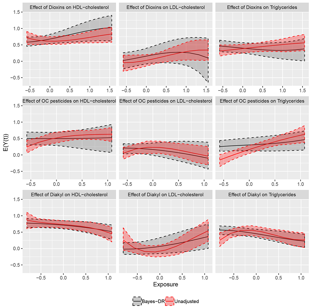
Estimated exposure response curves from the doubly robust estimator (black line) as well as the naïve curve (red line), which does not adjust for any covariates. This figure appears in color in the electronic version of this article, and any mention of color refers to that version.

7. Discussion

We have introduced an approach for causal inference that has a number of desirable features. First, it can be applied to doubly robust estimators of causal effects for binary or continuous treatments. This is particularly important as the literature on estimating the causal effect curve for continuous treatments is small, and has not been extended to high-dimensional scenarios. We showed that our approach maintains asymptotic properties such as double robustness, fast convergence rates, and consistent variance estimation, while achieving improved performance in finite samples. In particular, our inferential approach leads to nominal interval coverage when frequentist counterparts that rely on asymptotics fail to do so. Flexible Bayesian treatment and outcome models can be straightforwardly accommodated reducing the impact of model misspecification. While we focused on high-dimensional scenarios with spike and slab priors in this paper, the ideas presented apply to any modeling framework for the treatment and outcome models, and a number of estimands for which doubly-robust estimators exist. For example, even though we explored scenarios with homogeneous treatment effects, our approach is directly extendable to settings with heterogeneous treatment effects.

Doubly robust estimation was first introduced in the Bayesian framework in Saarela et al. (2016), although there has been some debate about whether an estimator of counterfactual outcomes can utilize the propensity score within the Bayesian framework (Robins et al., 2015). Robins and Ritov (1997) showed that a Bayesian analysis which honors the likelihood principle can not utilize the propensity score. In this paper, we do not attempt to address these concerns, nor do we propose a “fully” Bayesian approach. Our purpose has been to show that Bayesian methods coupled with doubly robust estimators provide flexible alternatives with desirable finite sample properties. This is even more important in high-dimensional scenarios where model uncertainty is high and relying on asymptotic approximations does not perform well.

Lastly, we ponder on why our approach to uncertainty quantification performs better in finite samples than existing approaches rooted in asymptotic theory. Asymptotic approaches rely on certain terms vanishing as the sample size increases, and ignoring these terms can lead to anti-conservative inference in small samples. In contrast, our inferential approach relies on combining posterior distributions with a resampling procedure. Uncertainty in our estimators stemming from parameter estimation is accounted for through the posterior distribution. While this requires the user to specify a prior distribution that can affect inference, we have shown that non-informative priors perform well, and importantly, posterior distributions reflect parameter uncertainty without relying on asymptotics. Our approach relies on asymptotics solely through our resampling procedure since the bootstrap is only valid asymptotically. Since the bootstrap is used in our approach to account for uncertainty stemming from the observed data for fixed values of the parameters, and the estimator has a simple form when the parameters are fixed, it is expected that the bootstrap performs well. As the sample size increases, any differences between our approach to inference and those rooted in asymptotics should dissipate.

References

- Antonelli J, Cefalu M, Palmer N, and Agniel D (2016). Doubly robust matching estimators for high dimensional confounding adjustment. Biometrics. [DOI] [PMC free article] [PubMed] [Google Scholar]
- Antonelli J, Parmigiani G, and Dominici F (2019). High-dimensional confounding adjustment using continuous spike and slab priors. Bayesian analysis 14, 805. [DOI] [PMC free article] [PubMed] [Google Scholar]
- Athey S, Imbens GW, and Wager S (2018). Approximate residual balancing: debiased inference of average treatment effects in high dimensions. Journal of the Royal Statistical Society: Series B (Statistical Methodology) 80, 597–623. [Google Scholar]
- Avagyan V and Vansteelandt S (2020). High-dimensional inference for the average treatment effect under model misspecification using penalised bias-reduced double-robust estimation. Biostatistics and Epidemiology, forthcoming . [Google Scholar]
- Bang H and Robins JM (2005). Doubly robust estimation in missing data and causal inference models. Biometrics 61, 962–973. [DOI] [PubMed] [Google Scholar]
- Belloni A, Chernozhukov V, and Hansen C (2014). Inference on treatment effects after selection among high-dimensional controls. The Review of Economic Studies 81, 608–650. [Google Scholar]
- Benkeser D, Carone M, Laan MVD, and Gilbert P (2017). Doubly robust nonparametric inference on the average treatment effect. Biometrika 104, 863–880. [DOI] [PMC free article] [PubMed] [Google Scholar]
- Chernozhukov V, Chetverikov D, Demirer M, Duflo E, Hansen C, Newey W, and Robins J (2018). Double/debiased machine learning for treatment and structural parameters. Econometrics Journal 21,. [Google Scholar]
- Daniel RM (2014). Double robustness. Wiley StatsRef: Statistics Reference Online pages 1–14. [Google Scholar]
- Dukes O, Avagyan V, and Vansteelandt S (2020). Doubly robust tests of exposure effects under high-dimensional confounding. Biometrics . [DOI] [PubMed] [Google Scholar]
- Ertefaie A, Asgharian M, and Stephens DA (2018). Variable selection in causal inference using a simultaneous penalization method. Journal of Causal Inference 6,. [Google Scholar]
- Farrell MH (2015). Robust inference on average treatment effects with possibly more covariates than observations. Journal of Econometrics 189, 1–23. [Google Scholar]
- Freedman D (1999). Wald lecture: On the bernstein-von mises theorem with infinite dimensional parameters. The Annals of Statistics 27, 1119–1141. [Google Scholar]
- Gill RD and Robins JM (2001). Causal inference for complex longitudinal data: the continuous case. Annals of Statistics pages 1785–1811. [Google Scholar]
- Hahn PR, Carvalho CM, Puelz D, He J, et al. (2018). Regularization and confounding in linear regression for treatment effect estimation. Bayesian Analysis 13, 163–182. [Google Scholar]
- Hirano K and Imbens GW (2004). The propensity score with continuous treatments. Applied Bayesian modeling and causal inference from incomplete-data perspectives 226164, 73–84. [Google Scholar]
- Kennedy EH, Ma Z, McHugh MD, and Small DS (2017). Non-parametric methods for doubly robust estimation of continuous treatment effects. Journal of the Royal Statistical Society: Series B (Statistical Methodology) 79, 1229–1245. [DOI] [PMC free article] [PubMed] [Google Scholar]
- Little RJ and Rubin DB (2000). Causal effects in clinical and epidemiological studies via potential outcomes: concepts and analytical approaches. Annual review of public health 21, 121–145. [DOI] [PubMed] [Google Scholar]
- Mitra R and Dunson D (2010). Two-level stochastic search variable selection in glms with missing predictors. The international journal of biostatistics 6,. [DOI] [PubMed] [Google Scholar]
- Ning Y, Sida P, and Imai K (2020). Robust estimation of causal effects via a high-dimensional covariate balancing propensity score. Biometrika 107, 533–554. [Google Scholar]
- Patel CJ, Cullen MR, Ioannidis JP, and Butte AJ (2012). Systematic evaluation of environmental factors: persistent pollutants and nutrients correlated with serum lipid levels. International journal of epidemiology 41, 828–843. [DOI] [PMC free article] [PubMed] [Google Scholar]
- Patel CJ and Ioannidis JP (2014). Studying the elusive environment in large scale. Jama 311, 2173–2174. [DOI] [PMC free article] [PubMed] [Google Scholar]
- Patel CJ, Pho N, McDuffie M, Easton-Marks J, Kothari C, Kohane IS, and Avillach P (2016). A database of human exposomes and phenomes from the us national health and nutrition examination survey. Scientific data 3,. [DOI] [PMC free article] [PubMed] [Google Scholar]
- Reich BJ, Storlie CB, and Bondell HD (2009). Variable selection in bayesian smoothing spline anova models: Application to deterministic computer codes. Technometrics 51, 110–120. [DOI] [PMC free article] [PubMed] [Google Scholar]
- Robins JM, Hernán MA, and Wasserman L (2015). On bayesian estimation of marginal structural models. Biometrics 71, 296. [DOI] [PMC free article] [PubMed] [Google Scholar]
- Robins JM and Ritov Y (1997). Toward a curse of dimensionality appropriate (coda) asymptotic theory for semi-parametric models. Statistics in medicine 16, 285–319. [DOI] [PubMed] [Google Scholar]
- Rosenbaum PR and Rubin DB (1983). The central role of the propensity score in observational studies for causal effects. Biometrika 70, 41–55. [Google Scholar]
- Saarela O, Belzile LR, and Stephens DA (2016). A bayesian view of doubly robust causal inference. Biometrika 103, 667–681. [Google Scholar]
- Shortreed SM and Ertefaie A (2017). Outcome-adaptive lasso: Variable selection for causal inference. Biometrics . [DOI] [PMC free article] [PubMed] [Google Scholar]
- Tan Z (2020a). Model-assisted inference for treatment effects using regularized calibrated estimation with high-dimensional data. Annals of Statistics 48, 811–837. [Google Scholar]
- Tan Z (2020b). Regularized calibrated estimation of propensity scores with model misspecification and high-dimensional data. Biometrika 107, 137–158. [Google Scholar]
- Van Der Laan MJ and Rubin D (2006). Targeted maximum likelihood learning. The International Journal of Biostatistics 2,. [DOI] [PMC free article] [PubMed] [Google Scholar]
- Watanabe S (2010). Asymptotic equivalence of bayes cross validation and widely applicable information criterion in singular learning theory. Journal of Machine Learning Research 11, 3571–3594. [Google Scholar]
- Wild CP (2005). Complementing the genome with an “exposome”: the outstanding challenge of environmental exposure measurement in molecular epidemiology. Cancer Epidemiology Biomarkers & Prevention 14, 1847–1850. [DOI] [PubMed] [Google Scholar]
- Wilson A, Zigler C, Patel C, and Dominici F (2018). Model-averaged confounder adjustment for estimating multivariate exposure effects with linear regression. Biometrics [DOI] [PMC free article] [PubMed] [Google Scholar]
Associated Data
This section collects any data citations, data availability statements, or supplementary materials included in this article.