Abstract
Although a variety of techniques have been developed to reduce the appearance of B-mode speckle, quantitative ultrasound (QUS) aims at extracting hidden properties of the tissue. Herein, we propose two novel techniques to accurately and precisely estimate two important QUS parameters, namely the average attenuation coefficient and the backscatter coefficient. Both techniques optimize a cost function that incorporates data and continuity constraint terms, which we call AnaLytical Global rEgularized BackscatteR quAntitative ultrasound (ALGEBRA). We propose two versions of ALGEBRA, namely 1D- and 2D-ALGEBRA. In 1D-ALGEBRA, the regularized cost function is formulated in the axial direction, and QUS parameters are calculated for one line of radiofrequency (RF) echo data. In 2D-ALGEBRA, the regularized cost function is formulated for the entire image, and QUS parameters throughout the image are estimated simultaneously. This simultaneous optimization allows 2D-ALGEBRA to “see” all the data before estimating QUS parameters. In both methods, we efficiently optimize the cost functions by casting it as a sparse linear system of equations. As a result of this efficient optimization, 1D-ALGEBRA and 2D-ALGEBRA are respectively 600 and 300 times faster than optimization using the dynamic programing method previously proposed by our group. In addition, the proposed technique has fewer input parameters that require manual tuning. Our results demonstrate that the proposed ALGEBRA methods substantially outperform least-squares and dynamic programming methods in estimating QUS parameters in phantom experiments.
Keywords: Quantitative ultrasound (QUS), Global QUS, Regularization, Attenuation, Backscatter coefficient
I. Introduction
As any imaging modality, ultrasound imaging has its own advantages and disadvantages. Although it is a real time, portable, and safe imaging modality, it provides a qualitative representation of the tissue, and as such, can be subject to different interpretations by different clinicians. Quantitative ultrasound (QuS) has emerged to resolve the aforementioned issue and quantitatively characterize tissue. Spectrum-based QUS techniques [1]–[4] investigate the Fourier transform of the radiofrequency (RF) data to estimate acoustic properties of tissue such as the effective scatterer diameter [5]–[10], scattering strength and acoustic concentration [3, 11], mean scatterer spacing [12]–[15], average attenuation αavg (average attenuation from intervening tissues) [16, 17], and backscatter coefficient σb [18]. Assessment of renal microstructure [4, 19, 20], fat infiltration [21, 24], structural evaluation of the uterine cervix during pregnancy [25, 26], and cancer therapy monitoring and assessment [27, 28] are some of its applications.
In addition to testing new clinical applications, a growing attention has focused on improving QUS techniques. Recent work has demonstrated that the accuracy and precision of backscatter QUS parameters can be improved by regularizing the depth variation of estimates of tissue properties, based on the hypothesis of piece-wise variability with depth [29]–[33] or by regularizing lateral and axial variation [34]. Moreover, our group recently showed that using dynamic programming (DP) substantially improves estimates of αeff and σb [35] compared to a least square (LSQ) method previously devised to estimate the same parameters [36]. LSQ and regularized algorithms based on DP were previously employed to estimate attenuation and BSCs. LSQ minimizes a cost function based on the squared-difference between the measured backscatter spectrum and a theoretical model to extract the values of the depth-averaged attenuation coefficient and the magnitude and frequency dependence of the backscatter coefficient. DP follows a similar strategy, but includes a regularization term in the cost function that assumes piece-wise continuity in the values of the depth-averaged attenuation and the magnitude and frequency dependence of the backscatter coefficient. To reduce the computational burden, the dynamic programing strategy stores minimized values of the cost function to avoid recomputing them at each spatial position.
However, the DP method faces three major issues:
1) It is a discrete optimization method. This means that the solution is based on minimizing the cost function from a set of discrete values defined by a search range and step size for the acoustic properties. A small step size improves the results by reducing the quantization error at the expense of increasing the computational complexity. This issue is exacerbated when processing a large field of view (i.e., abdominal or obstetric imaging). This limits the real-time applicability of DP. In addition, the step size must be defined by the user, adding to the complexity of its implementation.
2) A search range must be defined by the user. If ranges of values for the parameters of interest are not available for the tissue under study, a very large search range should be used, which further increases the computational complexity.
3) A fundamental problem of DP is that the graph formed by regularization costs must be a tree, and cannot have a cycle. As such, DP cannot consider the entire data. In other words, DP is applied on a 2D (axial vs lateral) array of power spectra but considers regularization only over depth for each lateral location independent from the others.
To cope with these issues, here we propose two versions of a novel technique which we call fast AnaLytical Global rEgularized BackscatteR quAntitative ultrasound, or ALGEBRA. ALGEBRA solves the regularized cost function analytically and does not need search ranges and step sizes. The first version of ALGEBRA, 1D-ALGEBRA, minimizes exactly the same cost function as DP [35], where 1D refers to regularization in one (axial) direction. The second version is called 2D-ALGEBRA and performs a global regularization in both axial and lateral directions. 1D- and 2D-ALGEBRA are inspired by state of the art regularization strategies used in ultrasound elastography [36, 37]. 1D- and 2D- ALGEBRA are about 600 times and 300 times faster than DP [35], respectively, and also provides more accurate and precise QUS estimates.
In the following sections, we describe the mathematical background of ALGEBRA. The performance of 1D- and 2D-ALGEBRA is compared with that of DP and LSQ on four tissue-mimicking phantoms. We demonstrate that both versions of ALGEBRA provide more accurate and precise estimates of the average attenuation and the backscatter coefficient than DP, and in a significantly shorter time.
II. ALGORITHMS
The application of ALGEBRA on QUS is based on the reference phantom method (RPM) [39] to provide system- and operator- independent QUS parameter estimation. According to the RPM, the ratio of the power spectrum Ss (f, z) of a sample s (phantom or tissue with unknown attenuation coefficient αs and backscatter coefficient σb,s) to the power spectrum Sr(f, z) of a reference phantom r (with known αr and σb,r, and similar sound speed to the sample, and where subscript r indicates “reference”) [40] can be modeled as:
| (1) |
where f, z, and x are frequency, depth, and lateral position, respectively. The factor A accounts for total attenuation of the acoustic pulse from the transducer to depth z:
| (2) |
where α is in Np.cm−1. Assuming that the attenuation coefficient varies linearly with frequency [35], i.e., α (f; z, x) = α0 (z, x) f, where α0 in Np.cm−1 MHz−1 is the specific attenuation as defined by the International Electrotechnical Commission [41], then the total attenuation Eq. (2) can be expressed as:
| (3) |
where αavg is the average attenuation equal to the average specific attenuation along the propagation depth z.
| (4) |
In the case of the homogeneous reference, the average attenuation αavg [cm−1 MHz−1] is equal to its local attenuation coefficient α0,r. Note that α, α0, and αavg can also be expressed in dB cm−1 or dB cm−1 MHz−1 by multiplying their numerical value by 8.686.
We employ a power law model to parameterize the frequency dependence of σb (f; z, x) as follows:
| (5) |
where β and ν indicate the value of the backscatter coefficient at 1MHz and its frequency dependence, respectively. After substituting Eqs. (2)–(4) into (1) and taking the natural logarithm from both sides similar to [35], we have:
| (6) |
where
| (7) |
Both 1D- and 2D-ALGEBRA make use of a cost function containing a data term, D, and a regularization term, R:
| (8) |
A. 1D-ALGEBRA
The ALGEBRA methods are applied to an NR × NC × NF power spectra matrix, where NR is the number of rows corresponding to different axial positions, NC is the number of columns corresponding to different lateral positions, and NF is the number of frequency bins within a useable frequency range. In 1D-ALGEBRA, one column (or lateral position) of power spectra is considered and regularization is performed in the axial direction to estimate a, b, and n at different axial positions along that column. In 2D-ALGEBRA, the entire array of power spectra is used in a 2D regularization strategy.
Removing the x dependence in (5), data and regularization terms D and R in 1D-ALGEBRA are defined as follows:
| (9) |
| (10) |
where i and l refer axial location and frequency indices, respectively. Index p refers to the three parameters (p = 1 for a, 2 for b, and 3 for n) and wp is the regularization weight for parameter p.
As Fig. 1(a) and Eq. (10) show, regularization is employed in the axial direction. To obtain the optimum parameters, we calculate the partial derivatives of the cost function with respect to ai, bi, an ni and set them to zero. After some manipulations, we arrive at a set of simple linear equation as follows:
| (11) |
Fig. 1.
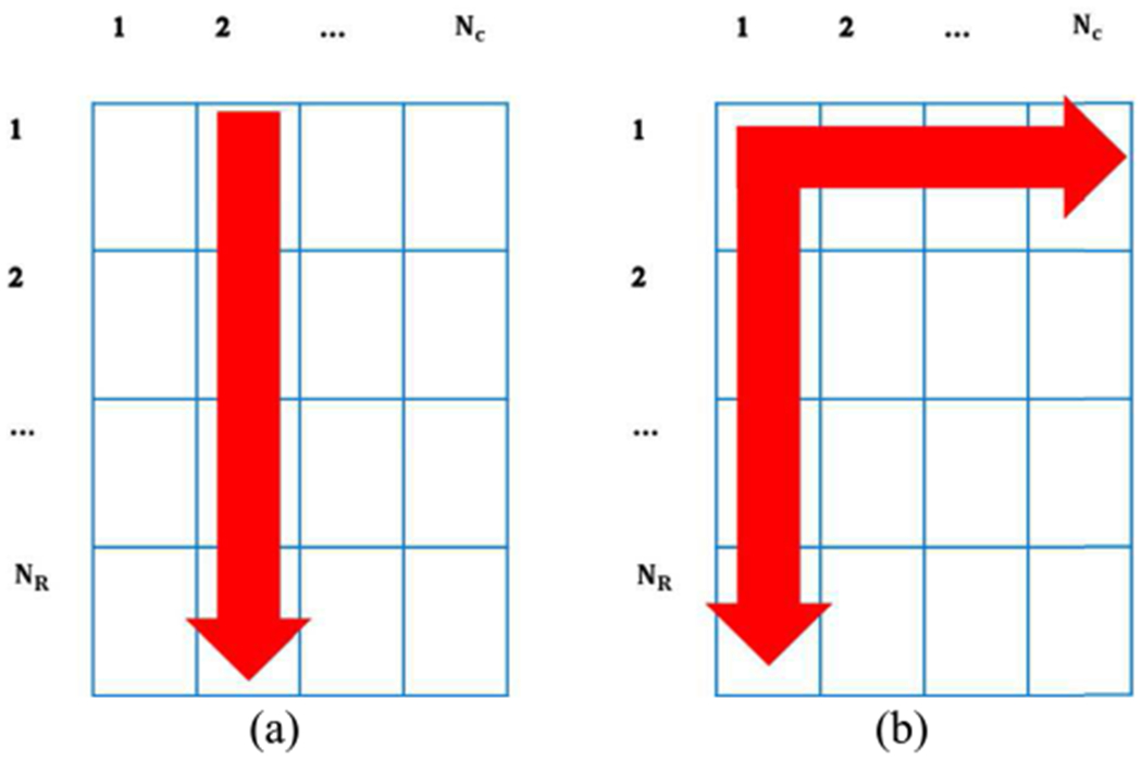
Regularization strategies for (a) 1D- and (b) 2D-ALGEBRA.
Y is a column vector with 3NR components containing the parameters to be estimated at different depths, i.e., ai, bi, an ni :
| (12) |
where superscript T indicates transposition. U is a 3NR × 3NR matrix which can be separated into two 3NR × 3NR matrices named C and W:
| (13) |
Matrix C is formed of 6 component matrices:
| (14) |
and Cj, j = 1, .., 6, are NR × NR diagonal matrixes:
| (15) |
where I is the NR × NR identity matrix and
| (16) |
Matrix W is defined as:
| (17) |
where Wa,Wb, and Wn are NR × NR matrices given by:
| (18) |
where
and O is a NR × NR matrix with zero elements.
T in (11) is a 3NR vector containing three vertically-concatenated NR × 1 column vectors, T1, T2, and T3 as follows:
| (19) |
whose ith components are given by:
| (20) |
The values of ai, bi, an ni at different depths are obtained by solving (11) for Y.
B. 2D-ALGEBRA
In 2D-ALGEBRA, we have similar data and regularization terms:
| (21) |
| (22) |
where j refers to the lateral location index. The indices of the regularization weights indicate (z) axial and (x) lateral directions. Thus, as Eq. (22) shows, the regularization is employed in both axial (z) and lateral (x) directions (Fig 1(b)).
For the 2D regularization the components of C have different sizes (NRNC × NRNC) as each component should also include lateral coefficient parameters. Therefore, the size of C will be 3NRNC × 3NRNC. The matrix components of W2 are defined as follows:
| (23) |
where
| (24) |
V is a NRNC × NRNC matrix defined as
| (25) |
where V1, V2, …, VNC are NR × NR matrices, and V2 = V3= … =VNC−1:
| (26) |
| (27) |
| (28) |
In (26) to (28), except for the first and last elements, all the elements of the main diagonal are repeated NR −2 times. The size of matrix ρ in Eq. (29) is NRNC × NRNC same as V.
The formulation of ρ is as follows:
| (29) |
where m1 and m2 are NR x NR matrices as follows. Matrix m1 is repeated NC times and matrix m2 is repeated NC − 1 times in each direction to form ρ.
| (30) |
| (31) |
Again, index p refers to the three parameters (p = 1 for a, 2 for b, and 3 for n). It is important to note that Eq. (24) has the same functional form for the three parameters a, b and n because it is expressed in terms of index p. However, the actual values of the matrix Wp2 are different for different values of p due to the different values of the weights wp1 and wp2. Here, we also have a similar T vector but with 3NRNC elements. After solving a similar equation to (11), we will solve for all 3NRNC parameters.
III. METHODS
A. Tissue-mimicking phantoms
1D- and 2D-ALGEBRA were tested to data acquired from five tissue mimicking phantoms with the following properties:
- Phantom A: Uniform
- α0,s = 0.654dBcm−1MHz−1
- βs = 1.02 × 10⁻⁶cm−1sr−1MHz−ν
- νs = 4.16
- σb,s(6.6MHz) = 2.62 × 10⁻³cm−1 sr−1
- Phantom B: Reference for Phantom A
- α0,s = 0.670dBcm−1MHz−1
- βs = 8.79 × 10⁻⁶cm−1sr−1MHz−ν
- νs = 3.14
- σb,s (6.6MHz) = 3.29 × 10⁻³cm−1sr−1
-
Phantom C: Attenuation step
Top and bottom layers:- α0,s = 0.510dBcm−1 MHz−1
- βs = 1.60 × 10⁻⁶cm−1sr−1MHz−ν
- νs = 3.52
- σb,s(8.9MHz) = 3.52 × 10⁻³cm−1sr−1
Middle layer:- α0,s = 0.779dBcm−1 MHz−1
- βs = 3.22 × 10⁻⁶cm−1sr−1MHz−ν
- νs = 3.13
- σb,s(8.9MHz) = 3.02 × 10⁻³cm−1 sr−1
-
Phantom D: Backscatter step
Top and bottom layers- α0,s = 0.554dBcm−1 MHz−1
- βs = 4.82 × 10⁻⁷cm−1sr−1MHz−ν
- νs = 3.80
- σb,s(8.9MHz) = 3.52 × 10⁻³cm−1 sr−1
Middle layer- α0,s = 0.58dB · cm−1MHz−1
- βs = 3.94 × 10⁻⁶cm−1sr−1MHz−ν
- νs = 3.38
- σb,s(8.9MHz) = 6.37 × 10⁻³cm−1sr−1
-
Phantom E: Inclusion phantom (Gammex 410SCG phantom (Gammex-SunNuclear, Middleton, WI)):
Background- α0,s = 0.5dBcm−1 MHz−1
- βs = 2.997 × 10⁻⁶cm−1sr−1 MHz−1
- νs = 3.34
- σb,s(8MHz) = 3.11 × 10⁻³cm−1sr−1
Inclusions- Three 8mm-diameter cylindrical inclusions with +12, +6 and −6dB scattering with respect to the background
More details about the composition of phantoms A-D are available in [34, 40].
Phantom A comprises a water-based agarose-propylene combined with filtered milk. Phantom B is composed of water-based agarose added by graphite powder. Both phantoms contain glass-beads with 5-43μm diameter as the source of scattering. The ground truth values were obtained with single element transducers to measure attenuation and backscatter coefficient utilizing narrowband substitution and broadband pulse-echo techniques, respectively [41, 42].
Phantoms C (uniform BSC) and D (uniform attenuation) are water-based phantoms with three layer phantoms composed of mixtures of gelatin and unfiltered milk. The concentration of scatterers in phantom C is 4g/L in all parts, while in phantom D the concentration of scatterers in the second layer is 8g/L which is 4 times more than the other two layers. On the other hand, molten gelatin and unfiltered milk have been mixed with the ratio of 2.1:1 in all layers in phantom D. This ratio in the middle layer of phantom C is 1:1 to increase its attenuation with respect to the first and third layer, where the ratio is 2.85:1 [40].
B. Data Acquisition
1). Homogenous Phantom:
Two phantoms (A and B above) were scanned with a 9L4 linear array transducer on a Siemens Acuson S3000 (Issaquah, WA) scanner operated at a 6.6MHz nominal center frequency to obtain 10 uncorrelated frames of RF data for each phantom [35]. Phantom B was used as reference for the characterization of phantom A. RF data was accessed through the Axius Direct Research Interface [41].
2). Layered Phantoms:
10 uncorrelated frames of RF data were acquired from Phantoms C and D, using their top layers as references. Both phantoms were scanned using a linear array transducer on a Siemens Acuson S2000 scanner operated at an 8.9MHz center frequency [36].
3). Different Echogenicity Phantom (Gammex phantom):
Phantom E was scanned using a Verasonics Vantage 128 system (Verasonics, Kirkland, WA) with a L11-5v transducer operated at 8MHz to obtain 10 uncorrelated frames of RF data. Uncorrelated frames from a homogeneous region of the same phantom were used as reference.
C. Power Spectra Estimation
We applied LSQ, DP, 1D- and 2D-ALGEBRA to 10 independent frames of RF echo data from each phantom. Parameter estimation regions of size 4mm ×4mm were swept axially and laterally over each frame with an overlap of 85%, computing at each position the echo signal power spectrum using a multitaper approach [44]. This procedure resulted in power spectra matrices with 40 columns and 74 rows in the uniform phantom, 86 columns and 108 rows in the layered phantoms, and 55 columns and 103 rows in Phantom E.
We have solved LSQ analytically. To apply DP, the following search ranges were used:
where min and max indices refer to the minimum and maximum ground truth values in the layered phantoms. These values were the same in the uniform phantom.
Tables I(A) and (B) show the regularization weights in each method. The weights of 1D-ALGEBRA are same as DP. The first and second elements of 2D-ALGEBRA weights correspond to the axial and lateral regularizations, respectively. In each method, first, the algorithm was executed using weights in order of 10. Then, considering the results, the weights were increased or decreased. The weights were increased when we saw a high variance in results, in other words when results were close to LSQ. On the other hand, weights were decreased when results were approaching a flat line. The values included in Table I(A) and (B) are the final ones.
TABLE I(A).
Regularization Weights In Four Phantoms
| DP | |||
|---|---|---|---|
| Phantom | wα | wb | wn |
| A | 1012 | 108 | 108 |
| C | 7×10⁶ | 101 | 6×10⁴ |
| D | 7×10⁸ | 3×101 | 104 |
| E | 8×10² | 8×10² | 8×10² |
TABLE I(B).
Regularization Weights In Four Phantoms
| 2D-ALGEBRA | |||
|---|---|---|---|
| Phantom | wα | wb | wn |
| A | [1010 1010] |
[108 108] |
[108 108] |
| C | [7×10⁶ 109] |
[101 101] |
[6×10⁴ 6×10⁴] |
| D | [7×10⁸ 7×10⁸] |
[3×101 3×101] |
[104 104] |
| E | [4×10² 4×10²] |
[4×10² 4×10²] |
[4×10² 4×10²] |
It can be easily shown that a symmetric diagonal dominant matrix, where its diagonal entries are positive, is a positive definite matrix. In addition, according to a theorem in linear algebra [45], the unique solution for equation Ax = b exists if and only if A (here, matrix U) is full rank. Therefore, as U is full rank, the unique solution exists. 1D- and 2D-ALGEBRA were implemented in Matlab R2018a (MathWorks, USA).
To obtain Y in Eq. (11), we use the mldivide function “\” in Matlab. This operator is time efficient and provides two algorithms for full and sparse inputs [46].
IV. Results
A. Phantom A
Figure 2(a) shows the mean and the standard deviation (error bars) of the attenuation coefficient (αs) vs. depth obtained from the 400 estimates using DP (green), 1D-ALGEBRA (blue), and 2D-ALGEBRA (red). The black dash line refers to the expected values. While 1D-ALGEBRA resulted in larger standard deviation compared to DP, the standard deviation obtained with 2D-ALGEBRA was close to that of DP.
Fig. 2.
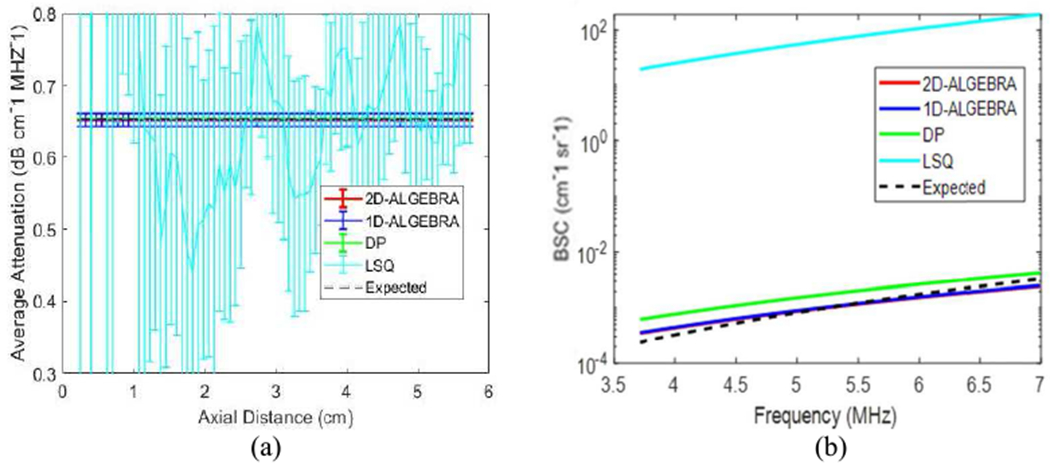
Results of 1D-ALGEBRA (blue), 2D-ALGEBRA (red), DP (green), and LSQ (cyan) in phantom A (uniform). The error bars show the standard deviation over the 400 samples for average attenuation coefficient (a) and reconstructed backscatter coefficient averaged over 400 samples (b). In (a), blue, red, cyan and black are superimposed. The black dashed line is the ground truth.
In Fig 2(b), the BSC is reconstructed from the average values of the 400 estimates of βs and νs. It can be observed that the bias of estimation using 1D- and 2D-ALGEBRA is lower than LSQ and DP.
Fig 3 shows the B-mode image of the phantom and parametric images of the reconstructed BSC evaluated at 6.6MHz in dB scale with respect to 10−4 cm−1 sr−1 using LSQ, DP, 1D- and 2D-ALGEBRA. In all phantoms, the range of color bar corresponds to the range of values obtained with DP. Visual comparison confirms that 1D- and 2D-ALGEBRA have the most similarity to ground truth compared to DP and LSQ. Quantitative analysis of bias and variance of BSC at center frequency reveals that using 1D-ALGEBRA leads to 98% decrease in variance and 39% in bias respect to DP. In addition, using 2D-ALGEBRA results in 100% and 35% reduction in variance and bias, respectively.
Fig. 3.
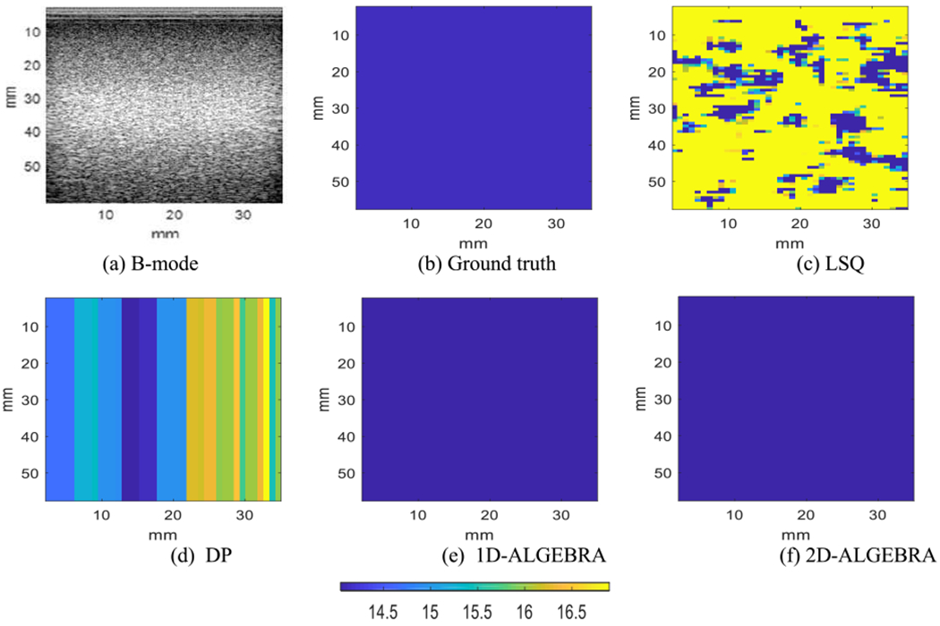
Parametric images of the backscatter coefficient at the center frequency in phantom A (uniform). Results are shown on a dB scale with respect to 10−4 cm−1 sr−1. The colorbar shows BSC at the center frequency.
To estimate the QUS parameters in an image with NC =74 and NR =40 using 1D- and 2D- ALGEBRA required 4 and 8 sec, respectively. In comparison, a Matlab implementation of DP required 2400 second for the same problem.
B. Phantoms C and D
Fig 4(a) and 4(b–d) show the average and standard deviation (error bars) over 860 estimates of αavg for Phantom C (attenuation step) and the results of the reconstruction of the backscatter coefficient from the average values of βs and νs in each layer using Eq. (5), respectively. In these figures, the black dashed line is the expected value of the parameter. In the case of the average attenuation (Fig 4(a)), there is a smooth transition from the top to the middle layer to do the averaging effect of Eq. (4). Also, the standard deviation of DP is lower than 1D-ALGEBRA. On the other hand, Fig 5 reveals that the step size in DP had not been small enough as we see each layer is not distinguished well. Here, to show how different layers are distinguished, we created a parametric image of the local attenuation (αlocal). The following equation shows how αlocal is obtained from αavg:
| (32) |
Fig 5(f) demonstrates that using 2D-ALGEBRA, αlocal estimation agrees well with ground truth. The analysis of bias and variance of local attenuation shows that 1D- and 2D-ALGEBRA yield 81% reduction in bias. The variance of DP results is small, but it should not be misinterpreted as we see the parametric image of DP is far from the ground truth. This is evidence of the drawbacks of DP referred to in the introduction section.
Fig. 4.
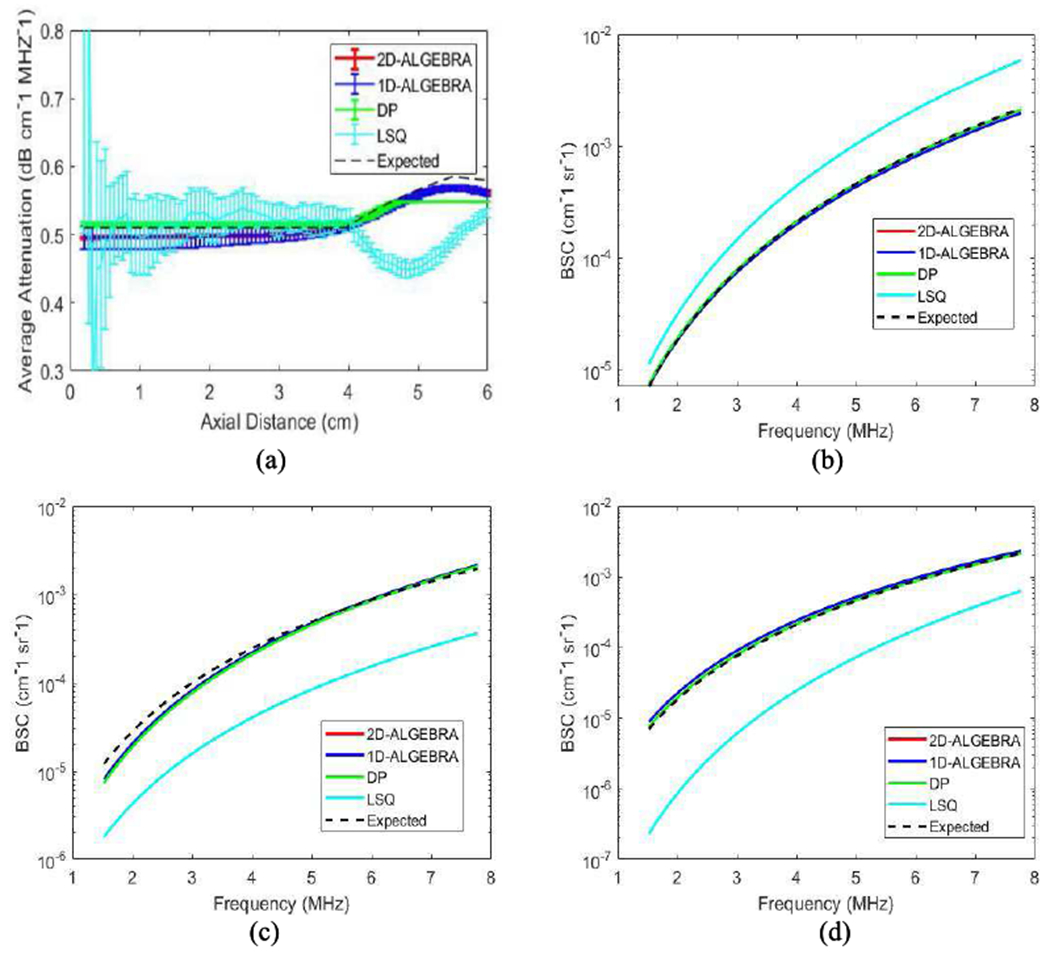
Results of 1D-ALGEBRA (blue), 2D-ALGEBRA (red), DP (green), and LSQ (cyan) in phantom C (attenuation step). The error bars show the standard deviation over the 860 samples for average attenuation coefficient (a) and reconstructed backscatter coefficient averaged over 400 samples in layer 1 (b), layer 2 (c), layer 3 (d). The black dashed line is the ground truth values. The red curve is superimposed by the blue curve.
Fig. 5.
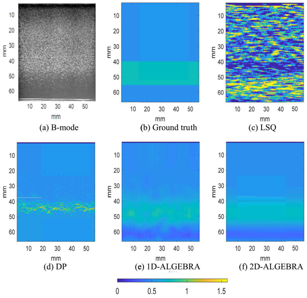
Parametric images of the local attenuation (computed from Eq. (30)) of phantom C (attenuation step). The color bar shows the value of local attenuation.
To estimate the QUS parameters in an image with NC =108 and NR =86 required 6 and 12 sec, respectively. In comparison, a Matlab implementation of DP required 3600 sec for the same problem.
Fig 6(a) shows the error bars over 860 estimate of αavg for phantom D (backscatter step) and Fig(6-d) shows results of the reconstruction of the backscatter coefficient from the average values of αs and νs in each layer.
Fig. 6.
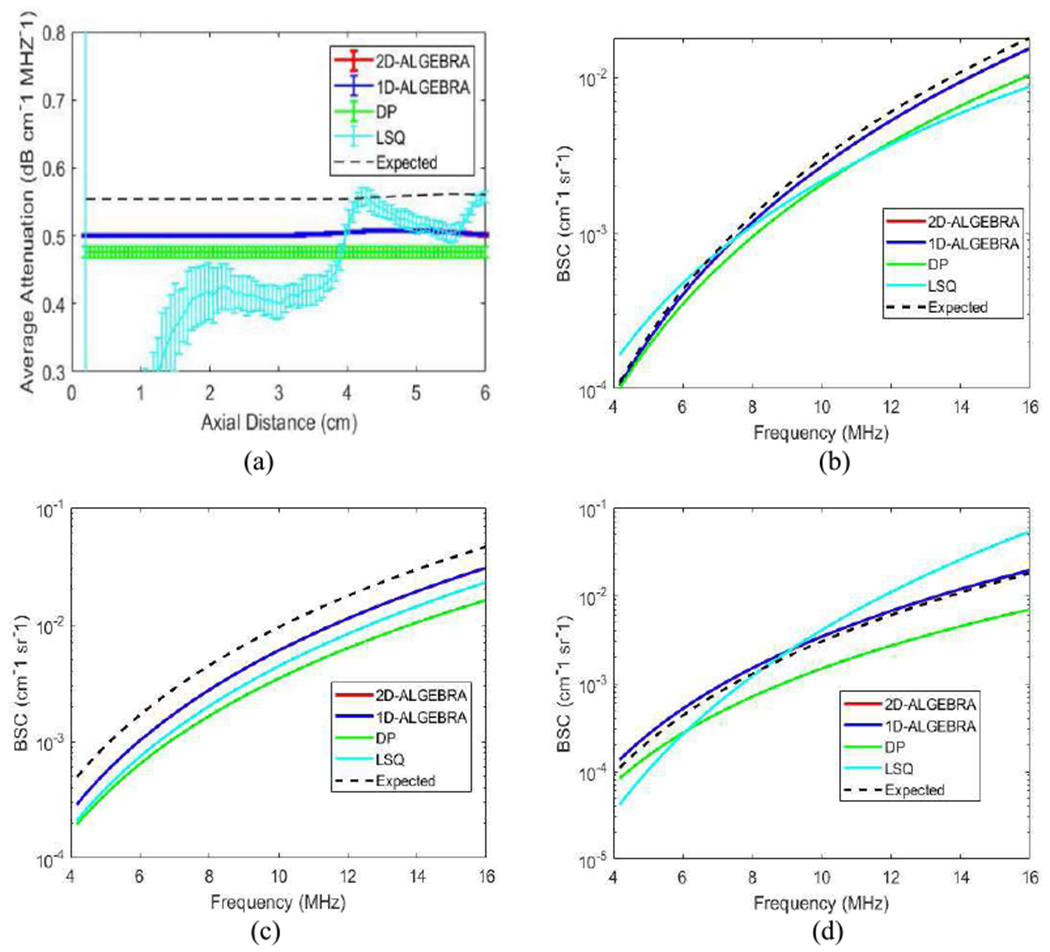
Results of 1D-ALGEBRA (blue), 2D-ALGEBRA (red), DP (green), and LSQ (cyan) in phantom D (backscatter step). The error bars show the standard deviation over the 860 samples for the average attenuation (a) and reconstructed backscatter coefficient averaged over 400 samples in layer 1 (b), layer 2 (c), layer 3 (d). The black dashed line is the expected value. The red curve is superimposed by the blue curve.
Fig. 7. shows the B-mode (a) and ground truth (b) as well as parametric images of backscatter coefficient obtained at the center frequency using LSQ (c), DP (d), 1D (e)- and 2D-ALGEBRA (f) in phantom D (backscatter step). Visual assessment confirms that 1D- and 2D-ALGEBRA outperform other methods. Quantitative assessments of BSC at central frequency disclose 88% reduction in variance as well as 56% in bias using 1D-ALGEBRA compared to DP. In addition, using 2D-ALGEBRA leads to 99% and 55% decrease in variance and bias compared to DP, respectively.
Fig. 7.
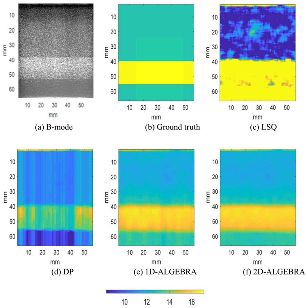
Parametric image of the backscatter coefficient at the center frequency of phantom D (backscatter step). Results are shown on a dB scale with respect to 10−4cm−1 sr−1
To estimate the QUS parameters in an image with NC =108 and NR =86 with 1D- and 2D-ALGEBRA took 9 and 18 sec, respectively. In comparison, a Matlab implementation of DP took 5400 second for the same problem.
C. Phantom E
Fig 8 shows the parametric image of BSC at the center frequency. Quantitative assessment of BSC at the center frequency reveals that using 1D-ALGEBRA leads to 35% reduction in bias in addition to 29% reduction in variance laterally compared to DP. Furthermore, using 2D-ALGEBRA yields 31% and 25% reduction in variance laterally and axially, respectively as well as 26% reduction in bias with respect to DP.
Fig. 8.
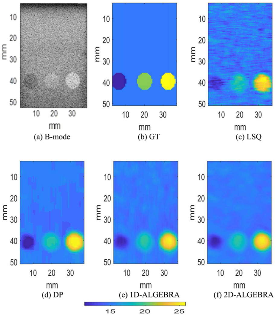
Parametric image of the backscatter coefficient at the center frequency of phantom E (inclusion phantom). Results are shown on a dB scale with respect to 10−4 cm−1 sr−1.
To estimate the QUS parameters in an image with NC =103 and NR =55, required 2 and 4 sec, respectively. In comparison, a Matlab implementation of DP took 1200 second for the same problem.
Figs 9(a) and (b) show two parametric images of phantom E using 1D-Algebra with two different sets of weights: [10, 10, 10] and [104, 104, 104], respectively. Fig 9(b) is smoother than Fig 9(a) (less variance), at the expense of blurring the edges of the inclusions (larger bias).
Fig. 9.
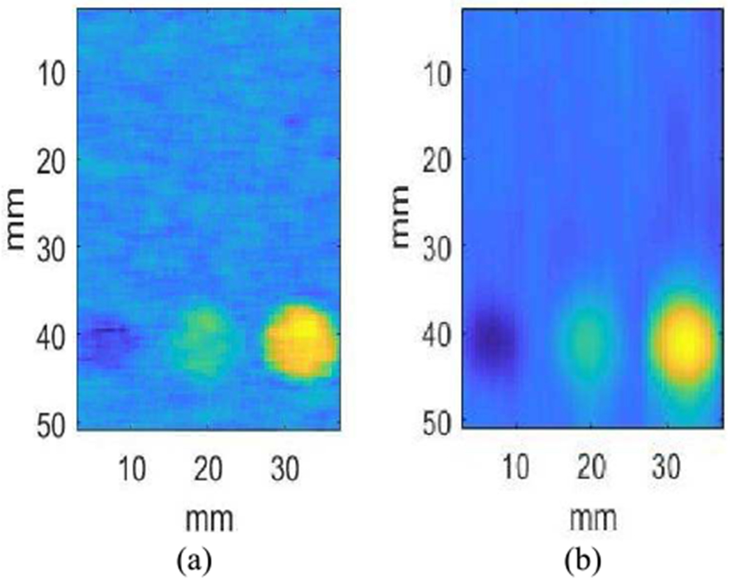
Influence of regularization weights in the parametric images of phantom E with 1D-ALGEBRA. Weights in (a): [10 10 10], weights in (b): [104 104 104].
V. Discussion
This work presented two analytical, regularized estimators of the attenuation and backscatter properties of tissue-mimicking materials. After various tests in tissue-mimicking phantoms, these algorithms, named 1D- and 2D-ALGEBRA, outperformed previously proposed regularized strategies (DP) in the following aspects:
Because of 1D- and 2D-ALGEBRA are analytical solutions to the minimization of a cost function, it does not require the definition of search ranges for the expected values of the parameters.
Contrary to DP, the attenuation and backscatter parameters can be estimated on a continuous scale.
Both 1D- and 2D-ALGEBRA are up to 600 times faster than DP.
Considering these advantages, ALGEBRA has great potential to be applied clinically.
Theoretically, we expect exactly the same result using DP and 1D-ALGEBRA as the cost functions are the same. However, achieving this requires step sizes to be small enough so that discontinuous ranges provided by DP be approximated by continuous range provided by 1D-ALGEBRA. On the other hand, as we are using a large number of samples, it is practically impossible to consider small step size for each parameter. For that reason, DP results are not as good as 1D-ALGEBRA. Nevertheless, 1D-ALGEBRA yields estimates with similar levels of bias and standard deviation than DP, but in a much shorter time.
Moreover, comparing 1D-ALGEBRA and 2D-ALGEBRA reveals that 2D-ALGEBRA outperforms 1D-ALGEBRA in terms of bias and variance as it exploits regularization in both axial and lateral directions. Comparing the backscatter coefficient estimation results shown in Fig 2, 4, 6(b–d) can result in the misleading conclusion that 1D-ALGEBRA and 2D-ALGEBRA provide almost the same results. This happens as we are plotting semi-log of . The improved performance of 2D-ALGEBRA compared to 1D-ALGEBRA is clear when 2D color-coded images are compared as shown in Figs 3, 5, and 7. In phantom A (uniform) shown in Fig 3, 2D-ALGEBRA leads to almost same estimations in all parts of the phantom. For the layered phantoms (Figs 5, 7) it can be seen that 2D-ALGEBRA can well distinguish three layers of phantoms C and D, especially in phantom D with the backscatter step.
This work has various limitations:
As shown in Eq. (10), the regularization term is based on an L2 norm. In a previous study based on dynamic programing, Vajihi et al. [47] showed that the use of L1 norm in the regularization terms provides better precision in parameter estimates than the use of L2 norm. However, the L1 norm is not analytically differentiable so it could not be implemented in ALGEBRA. Despite this limitation, we showed here that 1D- and 2D-ALGEBRA significantly improve the accuracy and precision of the parameter estimates over DP, probably due to the removal of the restriction of a discrete grid of parameter values over which the cost function is minimized.
The current implementation of ALGEBRA required adjusting the regularization weights to each phantom experiment. In general, larger weights are used in phantoms in which there is not a large change in the acoustic properties, such as phantom A, thus allowing a significant variance reduction. However, increasing the weights to reduce the variance can result in biased estimates. In other words, there is a trade-off between variance and bias in the selection of the weights. We are currently working on an automated method to select the weights based on identifying what acoustic properties are the most influential in the selection process. The weights that result from applying this method to representative data from various organ could be saved as part of the imaging presets in the scanner to provide ALGEBRA-based parametric images in real time. This is topic of our current research.
The attenuation coefficient was assumed to be linearly dependent on frequency. A more realistic model would be a power-law fit [48]. However, the effect of the power law dependence could be minimized by the averaging effect of the average attenuation. If a significant deviation from a linear dependence on frequency is expected, ALGEBRA could be applied over contiguous, narrow frequency bands over which the variation of the average attenuation with frequency could be approximated as linear, as implemented by Nasief et al. [49] Then, the values obtained from the various frequency bands could be combined.
The backscatter coefficient was parametrized in terms of a power law. We chose the power law to model the backscatter coefficient vs. frequency because (1) is the same model assumed in the LSQ and DP methods and (2) because the size of the scatterers in the phantoms were such that the product of the wave number and the scatterer radius is smaller than 0.5, which can lead to biased estimates of the scatterer size [50]. However, Eq. (5) could be modified to consider different scattering models, such as form factors for different scatterer geometries to estimate the effective scatterer size [6], and structure factor models to quantify scatterer volume fraction in cases of highly packed scatterers [51]. We have recently reported results on the modified DP to estimate effective scatterer size and acoustic concentration in tissue mimicking phantoms [52]. We are currently working on modifying ALGEBRA to estimate these parameters.
VI. Conclusion
In this study, two versions of an analytically-solved, regularized QUS estimation technique, 1D-ALGEBRA and 2D-ALGEBRA, were proposed to estimate the average attenuation as well as the magnitude and frequency dependence of the backscatter coefficient. 1D-ALGEBRA is the fast version of our previous DP method which applies an axially regularized cost function. On the other hand, 2D-ALGEBRA uses a globally (axially and laterally) regularized cost function. Regarding the quantitative analysis of bias and variance, we can conclude that applying 2D-ALGEBRA substantially improves the results compared to DP as it benefits the regularization in both axial and lateral directions.
Acknowledgment
This work was supported by the NSERC Discovery Grant RGPIN 04136, NIH R01HD072077, and UNAM PAPIIT IA102320.
Biographies
Noushin Jafarpisheh was born in Isfahan, Iran. She received her B.Sc. degree in electrical engineer from Isfahan University of Technology, Isfahan, Iran, her M.A.Sc. degree in electrical engineering from K.N.Toosi University of Technology, Tehran, Iran. She is currently pursuing her Ph.D. degree in electrical and computer engineering at Concordia University, Montreal, Canada.
Her research interests include, medical image processing, quantitative ultrasound, and machine learning.

Timothy J. Hall received the B.A. degree in physics from the University of Michigan–Flint, Flint, MI, USA, in 1983, and the M.S. and Ph.D. degrees in medical physics from the University of Wisconsin–Madison, Madison, WI, USA, in 1985 and 1988, respectively. From 1988 to 2002, he was with the Department of Radiology, University of Kansas Medical Center, Kansas City, KS, USA, where he worked on measurements of acoustic scattering in tissues, metrics of observer performance in ultrasound imaging, and developed elasticity imaging methods and phantoms for those and similar studies. In 2003, he returned to the University of Wisconsin–Madison, where he is a Professor and Interim Chair of the Department of Medical Physics. In 2019 he joined the leadership of the Quantitative Imaging Biomarker Alliance as Vice Chair of the organization. His research interests include developing new image formation strategies based on acoustic wave propagation and tissue viscoelasticity, the development of methods for system performance evaluation, and quantitative biomarker development and implementation.

Hassan Rivaz is an Associate Professor of Electrical and Computer Engineering at Concordia University. He received BSc degree from Sharif University of Technology, MASc from the University of British Columbia, and PhD from Johns Hopkins University.
He directs the IMPACT lab: IMage Processing And Characterization of Tissue, and is a Concordia University Research Chair in Medical Image Analysis. His research interests are medical image analysis, machine learning, deep learning, elastography and quantitative ultrasound.
He is an Associate Editor of IEEE Transactions on Medical Imaging (TMI), and IEEE Transactions on Ultrasonics, Ferroelectrics and Frequency Control (TUFFC). He is a member of the Organizing Committee of IEEE EMBC 2020 (Montreal, Canada), IEEE ISBI 2021 (Nice, France), and IEEE IUS 2023 (Montreal, Canada).
He has served as an Area Chair of MICCAI since 2017. He co-organized two tutorials on advances in ultrasound imaging at IEEE ISBI 2019 and 2018. He also co-organized the CURIOUS 2018 and CURIOUS 2019 Challenges on registration of ultrasound and MRI in neurosurgery, and the CereVis 2018 Workshop on Cerebral Data Visualization, all in conjunction with MICCAI.

Ivan M. Rosado-Mendez was born in Merida, Mexico. He received the B.S. degree in engineering physics from the Tecnologico de Monterrey, Monterrey, Mexico, in 2006, the M.S. degree in medical physics from the National Autonomous University of Mexico, Mexico City, Mexico, in 2009, and the Ph.D. degree in medical physics from the University of Wisconsin–Madison, Madison, WI, USA, in 2014. He is currently an Assistant Professor with the Department of Experimental Physics at the Institute of Physics, National Autonomous University of Mexico. His research interests include quantification of coherent and incoherent ultrasonic scattering for tissue characterization as well as the analysis of tissue viscoelasticity using shear wave elastography.
References
- [1].Lizzi FL, Greenebaum M, Feleppa EJ, Elbaum M, and Coleman DJ, “Theoretical framework for spectrum analysis in ultrasonic tissue characterization,” J. Acoust. Soc. Am, vol. 73, no. 4, pp. 1366–1373, 1983. [DOI] [PubMed] [Google Scholar]
- [2].Lizzi FL, Ostromogilsky M, Feleppa EJ, Rorke MC, and Yaremko MM, “Relationship of ultrasonic spectral parameters to features of tissue microstructure,” IEEE Trans. Ultrason. Ferroelectr. Freq. Control, vol. 34, no. 3, pp. 319–329, 1987. [DOI] [PubMed] [Google Scholar]
- [3].Insana MF and Hall TJ, “Characterising the microstructure of random media using ultrasound,” Phys. Med. Biol, vol. 35, no. 10, pp. 1373–1386, 1990. [DOI] [PubMed] [Google Scholar]
- [4].Insana MF, Hall TJ, and Fishback JL, “Identifying acoustic scattering sources in normal renal parenchyma from the anisotropy in acoustic properties,” Ultrasound Med. Biol, vol. 17, no. 6, pp. 613–626, 1991. [DOI] [PubMed] [Google Scholar]
- [5].Insana MF, Hall TJ, Wood JG, and Yan ZY, “Renal ultrasound using parametric imaging techniques to detect changes in microstructure and function,” Invest. Radiol, vol. 28, no. 8, pp. 720–725, 1993. [DOI] [PubMed] [Google Scholar]
- [6].Insana MF, Wagner RF, Brown DG, and Hall TJ, “Describing small-scale structure in random media using pulse-echo ultrasound,” J. Acoust. Soc. Am, vol. 87, no. 1, pp. 179–192, 1990. [DOI] [PMC free article] [PubMed] [Google Scholar]
- [7].Oelze ML and Zachary JF, “Examination of cancer in mouse models using high-frequency quantitative ultrasound,” Ultrasound Med. Biol, vol. 32, no. 11, pp. 1639–1648, 2006. [DOI] [PubMed] [Google Scholar]
- [8].Nasief HG, Rosado-Mendez IM, Zagzebski JA, and Hall TJ, “A quantitative ultrasound-based multi-parameter classifier for breast masses,” Ultrasound Med. Biol, vol. 45, no. 7, pp. 1603–1616, 2019. [DOI] [PMC free article] [PubMed] [Google Scholar]
- [9].Sadeghi-Naini A et al. , “Breast-lesion characterization using textural features of quantitative ultrasound parametric maps,” Sci. Rep, vol. 7, no. 1, pp. 1–10, 2017. [DOI] [PMC free article] [PubMed] [Google Scholar]
- [10].Coila A, Torres G, Rouyer J, Aristizabal S, Urban M, and Lavarello R, “Recent developments in spectral-based ultrasonic tissue characterization,” in 2018 IEEE 15th International Symposium on Biomedical Imaging (ISBI 2018), 2018, pp. 1018–1021. [Google Scholar]
- [11].Mamou J, Oelze ML, O’Brien WD Jr, and Zachary JF, “Identifying ultrasonic scattering sites from three-dimensional impedance maps,” J. Acoust. Soc. Am, vol. 117, no. 1, pp. 413–423, 2005. [DOI] [PubMed] [Google Scholar]
- [12].Wear KA, Wagner RF, Insana MF, and Hall TJ, “Application of autoregressive spectral analysis to cepstral estimation of mean scatterer spacing,” IEEE Trans. Ultrason. Ferroelectr. Freq. Control, vol. 40, no. 1, pp. 50–58, 1993. [DOI] [PubMed] [Google Scholar]
- [13].Zhou Z, Wu W, Wu S, Jia K, and Tsui P,H, “A Review of Ultrasound Tissue Characterization with Mean Scatterer Spacing,” Ultrason. Imaging, vol. 39, no. 5, pp. 263–282, 2017. [DOI] [PubMed] [Google Scholar]
- [14].Nizam NI, Ara SR, and Hasan MK, “Classification of breast lesions using quantitative ultrasound biomarkers,” Biomed. Signal Process. Control, vol. 57, p. 101786, 2020. [Google Scholar]
- [15].Pereira WCA, Bridal SL, Coron A, and Laugier P, “Mean scatterer spacing of backscattered ultrasound signals from in vitro human cancellous bone specimens,” in 2002 IEEE Ultrasonics Symposium, 2002. Proceedings., 2002, vol. 2, pp. 1337–1340. [Google Scholar]
- [16].Gong P, Song P, Huang C, Trzasko J, and Chen S, “System-independent ultrasound attenuation coefficient estimation using spectra normalization,” IEEE Trans. Ultrason. Ferroelectr. Freq. Control, vol. 66, no. 5, pp. 867–875, 2019. [DOI] [PMC free article] [PubMed] [Google Scholar]
- [17].Nam K, Zagzebski JA, and Hall TJ, “Quantitative assessment of in vivo breast masses using ultrasound attenuation and backscatter,” Ultrason. Imaging, vol. 35, no. 2, pp. 146–161, 2013. [DOI] [PMC free article] [PubMed] [Google Scholar]
- [18].Ghoshal G, Mamou J, and Oelze ML, “State of the art methods for estimating backscatter coefficients,” in Mamou J and Oelze ML (eds) Quantitative ultrasound in soft tissues, Springer: Dordrecht, 2013, pp. 3–19. [Google Scholar]
- [19].Insana MF, Wood JG, and Hall TJ, “Identifying acoustic scattering sources in normal renal parenchyma in vitro by varying arterial and ureteral pressures,” Ultrasound Med. Biol, vol. 18, no. 6–7, pp. 587–599, 1992. [DOI] [PubMed] [Google Scholar]
- [20].Garra BS et al. , “Quantitative ultrasonic detection of parenchymal structural change in diffuse renal disease,” Invest. Radiol, vol. 29, no. 2, pp. 134–140, 1994. [DOI] [PubMed] [Google Scholar]
- [21].Nguyen TN et al. , “Characterizing Fatty Liver in vivo in Rabbits, Using Quantitative Ultrasound,” Ultrasound Med. Biol, vol. 45, no. 8, pp. 2049–2062, 2019. [DOI] [PMC free article] [PubMed] [Google Scholar]
- [22].Han A, Erdman JW, Simpson DG, Andre MP, and O’Brien WD, “Early detection of fatty liver disease in mice via quantitative ultrasound,” in 2014 IEEE International Ultrasonics Symposium, 2014, pp. 2363–2366. [Google Scholar]
- [23].Ghoshal G, Lavarello RJ, Kemmerer JP, Miller RJ, and Oelze ML, “Ex vivo study of quantitative ultrasound parameters in fatty rabbit livers,” Ultrasound Med. Biol, vol. 38, no. 12, pp. 2238–2248, 2012. [DOI] [PMC free article] [PubMed] [Google Scholar]
- [24].Lin SC et al. , “Noninvasive diagnosis of nonalcoholic fatty liver disease and quantification of liver fat using a new quantitative ultrasound technique,” Clin. Gastroenterol. Hepatol, vol. 65, no. 11, pp. 2042–2053, 2015. [DOI] [PMC free article] [PubMed] [Google Scholar]
- [25].Guerrero QW, Feltovich H, Rosado-Mendez IM, Carlson LC, Li G, and Hall TJ, “Anisotropy and spatial heterogeneity in quantitative ultrasound parameters: Relevance to the study of the human cervix,” Ultrasound Med. Biol, vol. 44, no. 7, pp. 1493–1503, 2018. [DOI] [PMC free article] [PubMed] [Google Scholar]
- [26].Guerrero QW, Feltovich H, Rosado-Mendez IM, Carlson LC, and Hallcor TJ, “Quantitative Ultrasound Biomarkers Based on Backscattered Acoustic Power: Potential for Quantifying Remodeling of the Human Cervix during Pregnancy,” Ultrasound Med. Biol, vol. 45, no. 2, pp. 429–439, 2019. [DOI] [PMC free article] [PubMed] [Google Scholar]
- [27].Oelze ML, Kemmerer JP, Ghoshal G, and Vlad RM, “Therapy monitoring and assessment using quantitative ultrasound,” in Quantitative Ultrasound in Soft Tissues, Springer, 2013, pp. 193–216. [Google Scholar]
- [28].Oelze ML, “Quantitative ultrasound successes: past, present and future,” in Medical Imaging 2020: Ultrasonic Imaging and Tomography, 2020, vol. 11319, p. 113190X. [Google Scholar]
- [29].Coila AL and Lavarello R, “Regularized spectral log difference technique for ultrasonic attenuation imaging,” IEEE Trans. Ultrason. Ferroelectr. Freq. Control, vol. 65, no. 3, pp. 378–389, 2018. [DOI] [PubMed] [Google Scholar]
- [30].Deeba F et al. , “SWTV-ACE: spatially weighted regularization based attenuation coefficient estimation method for hepatic steatosis detection,” in International Conference on Medical Image Computing and Computer-Assisted Intervention, Springer; 2019, pp. 610–618. [Google Scholar]
- [31].Destrempes F, Gesnik M, and Cloutier G, “Construction of adaptively regularized parametric maps for quantitative ultrasound imaging,” in 2019 IEEE International Ultrasonics Symposium (IUS), 2019, pp. 2027–2030. [Google Scholar]
- [32].Coila A et al. , “In vivo attenuation estimation in human thyroid nodules using the regularized spectral log difference technique: Initial pilot study,” in 2017 IEEE International Ultrasonics Symposium (IUS), 2017, pp. 1–4. [Google Scholar]
- [33].Saavedra AC, Coila A, Arroyo J, Castaneda B, and Lavarello RJ, “In vivo attenuation coefficient estimation in the healthy forearm and thigh human dermis,” in 2018 IEEE International Ultrasonics Symposium (IUS), 2018, pp. 1–4. [Google Scholar]
- [34].A B. and Hector Chahuaray RL, “Regularized framework for simultaneous estimation of ultrasonic attenuation and backscatter coefficients,” in IEEE International Ultrasonics Symposium (IUS), Accepted, 2020. [Google Scholar]
- [35].Vajihi Z, Rosado-Mendez IM, Hall TJ, and Rivaz H, “Low Variance Estimation of Backscatter Quantitative Ultrasound Parameters Using Dynamic Programming,” IEEE Trans. Ultrason. Ferroelectr. Freq. Control, vol. PP, no. 1, p. 1, 2018. [DOI] [PMC free article] [PubMed] [Google Scholar]
- [36].Nam K, Zagzebski JA, and Hall TJ, “Simultaneous backscatter and attenuation estimation using a least squares method with constraints,” Ultrasound Med. Biol, vol. 37, no. 12, pp. 2096–2104, 2011. [DOI] [PMC free article] [PubMed] [Google Scholar]
- [37].Rivaz H, Boctor EM, Choti MA, and Hager GD, “Real-time regularized ultrasound elastography,” IEEE Trans. Med. Imaging, vol. 30, no. 4, pp. 928–945, 2011. [DOI] [PubMed] [Google Scholar]
- [38].Hashemi HS and Rivaz H, “Global time-delay estimation in ultrasound elastography,” IEEE Trans. Ultrason. Ferroelectr. Freq. Control, vol. 64, no. 10, pp. 1625–1636, 2017. [DOI] [PubMed] [Google Scholar]
- [39].Yao LX, Zagzebski JA, and Madsen EL, “Backscatter coefficient measurements using a reference phantom to extract depth-dependent instrumentation factors,” Ultrason. Imaging, vol. 12, no. 1, pp. 58–70, 1990. [DOI] [PubMed] [Google Scholar]
- [40].Nam K et al. , “Comparison of ultrasound attenuation and backscatter estimates in layered tissue-mimicking phantoms among three clinical scanners,” Ultrason. Imaging, vol. 34, no. 4, pp. 209–221, 2012. [DOI] [PMC free article] [PubMed] [Google Scholar]
- [41].Commission IE, “Ultrasonics-Pulse-echo scanners: Part 2. Measurement of maximum depth of penetration and local dynamic range,” International Electrotechnical Commission, pp. 61391–61392, 2010. [Google Scholar]
- [42].Madsen EL et al. , “Interlaboratory comparison of ultrasonic backscatter, attenuation, and speed measurements.,” J. Ultrasound Med, vol. 18, no. 9, pp. 615–631, 1999. [DOI] [PubMed] [Google Scholar]
- [43].Chen J-F, Zagzebski JA, and Madsen EL, “Tests of backscatter coefficient measurement using broadband pulses,” IEEE Trans. Ultrason. Ferroelectr. Freq. Control, vol. 40, no. 5, pp. 603–607, 1993. [DOI] [PubMed] [Google Scholar]
- [44].Rosado-Mendez IM, Nam K, Hall TJ, and Zagzebski JA, “Task-oriented comparison of power spectral density estimation methods for quantifying acoustic attenuation in diagnostic ultrasound using a reference phantom method,” Ultrason. Imaging, vol. 35, no. 3, pp. 214–234, 2013. [DOI] [PMC free article] [PubMed] [Google Scholar]
- [45].Strang G and Borre K, Linear algebra, geodesy, and GPS. Siam, 1997. [Google Scholar]
- [46].“mldivide, \.” [Online]. Available: https://www.mathworks.com/help/matlab/ref/mldivide.html.
- [47].Vajihi Z, Rosado-Mendez I, Hall TJ, and Rivaz H, “L1 and l2 norm depth-regularized estimation of the acoustic attenuation and backscatter coefficients using dynamic programming,” in 2019 IEEE 16th International Symposium on Biomedical Imaging (ISBI 2019), 2019, pp. 1749–1752. [Google Scholar]
- [48].Szabo TL, Diagnostic ultrasound imaging: inside out. Academic Press, 2004. [Google Scholar]
- [49].Nasief HG, Rosado-Mendez IM, Zagzebski JA, and Hall TJ, “Acoustic properties of breast fat,” J. Ultrasound Med, vol. 34, no. 11, pp. 2007–2016, 2015. [DOI] [PMC free article] [PubMed] [Google Scholar]
- [50].Insana MF and Hall TJ, “Parametric ultrasound imaging from backscatter coefficient measurements: image formation and interpretation,” Ultrason. Imaging, vol. 12, no. 4, pp. 245–267, 1990. [DOI] [PubMed] [Google Scholar]
- [51].Franceschini E, Guillermin R, Tourniaire F, Roffino S, Lamy E, and Landrier J-F, “Structure factor model for understanding the measured backscatter coefficients from concentrated cell pellet biophantoms,” J. Acoust. Soc. Am, vol. 135, no. 6, pp. 3620–3631, 2014. [DOI] [PubMed] [Google Scholar]
- [52].Jafarpisheh N, Rosado-Mendez IM, Hall TJ, and Rivaz H, “Regularized Estimation of Effective Scatterer Size and Acoustic Concentration Quantitative Ultrasound Parameters Using Dynamic Programming,” in 42nd Annual International Conference of the IEEE Engineering in Medicine and Biology Society (EMBC), 2020. [DOI] [PMC free article] [PubMed] [Google Scholar]


