Abstract
In this paper, we establish daily confirmed infected cases prediction models for the time series data of America by applying both the long short-term memory (LSTM) and extreme gradient boosting (XGBoost) algorithms, and employ four performance parameters as MAE, MSE, RMSE, and MAPE to evaluate the effect of model fitting. LSTM is applied to reliably estimate accuracy due to the long-term attribute and diversity of COVID-19 epidemic data. Using XGBoost model, we conduct a sensitivity analysis to determine the robustness of predictive model to parameter features. Our results reveal that achieving a reduction in the contact rate between susceptible and infected individuals by isolated the uninfected individuals, can effectively reduce the number of daily confirmed cases. By combining the restrictive social distancing and contact tracing, the elimination of ongoing COVID-19 pandemic is possible. Our predictions are based on real time series data with reasonable assumptions, whereas the accurate course of epidemic heavily depends on how and when quarantine, isolation and precautionary measures are enforced.
Keywords: COVID-19, LSTM, XGBoost, Time series data
Introduction
The ongoing outbreak respiratory disease COVID-19 is caused by the novel coronavirus SARS-CoV-2 which happened at the end of 2019 till nowadays, has spread out all over the world and puts tremendous pressure on the economy and society. It was declared as global pandemic by World Health Organization (WHO) on March 11th 2020. Various emergency measures, such as regional lockdown, mass testing, issuing masks, have been taken by many countries to reduce the transmission and control the epidemic. The crucial problems are whether investments in medical services and prevention steps taken are effective in managing the spread of disease, and how the number of confirmed cases will grow in the future.
As the number of cases increases and more data becomes available, various researches [1], [2], [3], [4], [5], [6], [7] develop a range of mathematical models or employ machine learning algorithms to forecast the transmission of SARS-CoV-2. Previous studies have also employed LSTM [8], [9], [10], [11], [12] or XGBoost [13], [14], [15], [16], [17], [18], [19] models to forecast the spread of COVID-19 and identify the most influential COVID-19 indicators. Chimmua et al. [8] adopted LSTM algorithm to forecast confirmed cases in Canada within next two weeks and emphasized the significant role of social distance regular. Tomar and Gupta [9] utilized LSTM and curve fitting to forecast the number of COVID-19 cases in India for the next 30 days, as well as the influence of preventative measures such as social isolation and lockdown on the spread of COVID-19. Wang et al. [10] focused on predicting the long-term pandemic pattern of COVID-19 employing LSTM networks and a rolling update mechanism. In [11], the implementation of LSTM layers following the proposed convolutional neural network (CNN) block improves the 4-score disease severity prediction performance. Gautam [12] applied transfer learning to LSTM network models to anticipate additional COVID cases and fatalities. Models developed on data from early COVID infected nations such as Italy and the United States are used to predict the development of the disease in other nations. The machine learning algorithm XGBoost was employed to build the models to predict the criticality [13], mortality [14], [15] and survival [16] in COVID-19 patients. Li et al. [17] constructed an XGBoost-based classification algorithm to distinguish between influenza and COVID-19 patients. To quantify the impact of the COVID-19 pandemic on driving behavior, the authors [18] utilized explanatory XGBoost feature importance to evaluate the influence of COVID-19 and used seasonal ARIMA models to model. Kukar et al. [19] used random forest, deep neural networks, and XGBoost algorithms to build models that predicted COVID-19 diagnosis based on regular blood test results, age, and gender. To the best of our knowledge, few studies have used the combined LSTM networks and XGBoost models to predict infectious diseases in time series analysis.
Multiple studies have demonstrated the human-to-human transmission of COVID-19 through droplets and direct contact after analyzing the clinical characteristics of COVID-19 [20], [21], [22]. Experience with the monitoring of epidemics in various countries shows that there is a need for wide-ranging social distancing regulations [23], [24]. Based on the confirmed cases before January 1, 2020 in China, Li et al. [25] estimated the mean incubation period of COVID-19 is days, with the 95th percentile of the distribution at days, and the basic reproduction number is estimated to be . Guan et al. [26] obtained the median incubation period is 4 days (interquartile range, 2 to 7) according to the confirmed cases reported to the National Health Commission of China between December 11, 2019 and January 29, 2020. Lauer et al. [27] got the median incubation period is days, and infection cases develop symptoms within days based the confirmed cases reported between January 4, 2020 and February 24, 2020 from 50 provinces, regions, and countries. In [28], the authors indicated that control measures taken in China had an effect on COVID-19 transmissibility roughly 2 weeks after they were implemented. Hence, the majority of individuals will be diagnosed with symptoms within 14 days after being infected.
Depending on the characteristics of COVID-19 disease transmission, we built a mathematical model based on the following assumptions:
(A1) The number of confirmed cases is determined by the transmission force of infectious disease, such as the basic reproduction number, the probability of contact between the susceptible and infected individuals, and the investment in prevention and control resources, such as quarantine, isolation and precautionary measures are enforced.
(A2) The time series data of daily new confirmed cases provide information on the force of infection and investment in the prevention resources of epidemics. This information will not dramatically change in the short term and will have an effect on the number of new infections in the future. Using these time series data, it is possible to forecast the number of daily new confirmed cases in the near future. In other words, the number of daily new confirmed cases relates to historical data.
(A3) The majority of infectious individuals will be diagnosed within 14 days due to symptoms or large-scale monitoring. Confirmed individuals who are diagnosed will be isolated and treated, then they will lose the ability to infect.
(A4) Workplace transmission is a critical route of COVID-19 disease transmission. The number of new confirmed cases is correlated with the day of the week.
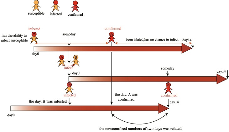
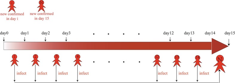
It can be assumed from assumption (A3) that infected individual who has not been diagnosed with a large-scale test can infect susceptible individuals during the incubation period. The duration of the infection of COVID-19 infected individuals would be shortened by increasing the scale of testing measures. Many infectious individuals have the potential to transmit COVID-19 disease within 14 days of infection, and the duration of infection in COVID-19 infected individuals is no more than 14 days. New confirmed individuals are affected by person who had been diagnosed within the previous 14 days. The daily number of new confirmed COVID-19 cases is linked to the number of new confirmed individuals in the previous 14 days (see Fig. 1, Fig. 2 ).
Fig. 1.
Schematic of the disease transmission. It indicates that the duration of infection in infected individuals with COVID-19 does not exceed 14 days.
Fig. 2.
Schematic of the relation between new confirmed individuals and the number of confirmed cases in the previous 14 days.
According to assumptions (A1)-(A4), we find the important features to establish a prediction model, which is shown in Fig. 3 . In the figure, mean represents the average number of new confirmed COVID-19 cases in the previous two weeks, which is used to describe the average level of disease transmission force and investment in epidemic control resources in the near future; Std measures the standard deviation of new confirmed cases in the previous two weeks, and is used to reflect recent variations in disease transmission force and investment in epidemic control resources; week is used to decide if the day is a working day. Taking the number of new infected COVID-19 cases in America as an example, a predictive model based on time series dataset is proposed that combines the LSTM and XGBoost machine learning algorithms, which can deal with time series data and extract features from previous data.
Fig. 3.
Schematic of the model features.
According to the discussion above, in this paper, we mainly focus on forecasting the growth of COVID-19 based on past transmission data and through hypothesis analysis. The paper is organized as follows. In Section “Methods”, we illustrate the mechanism of LSTM and XGBoost algorithms for the prediction of COVID-19 disease. A description of dataset collection and preparation is presented in Section “Materials”. The experimental results and comparative performance of the proposed machine learning model are provided in Section “Experimental results analysis”. Section “Conclusion and discussion” gives a brief conclusion and remarks.
Methods
LSTM
LSTM is an artificial Recurrent Neural Network (RNN) architecture used in the field of deep learning. It is an efficient algorithm to construct a sequential time series model.
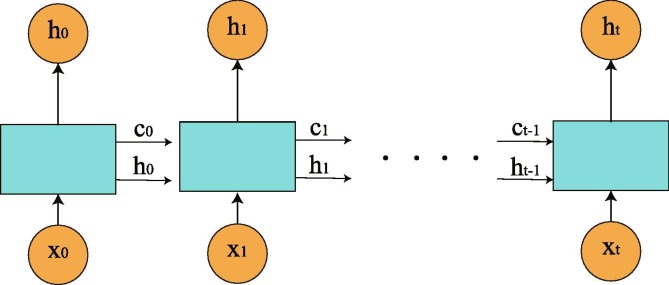
It’s well known that RNN is a class of artificial neural networks where connections between nodes form a directed graph along a temporal sequence. This allows RNN to exhibit temporal dynamic behavior. RNNs can use their internal state (memory) to process variable length sequences of inputs. A RNN can be thought of as multiple copies of the same network, each passing a message to a successor (see Fig. 4 ). They might be able to connect previous information to the present task. However, as that gap grows, RNNs become unable to learn to connect the information. The short-term memory problem of RNN is that short-term memory has a greater impact, but long-term memory has a small impact.
Fig. 4.
An unrolled RNN contains a single layer.
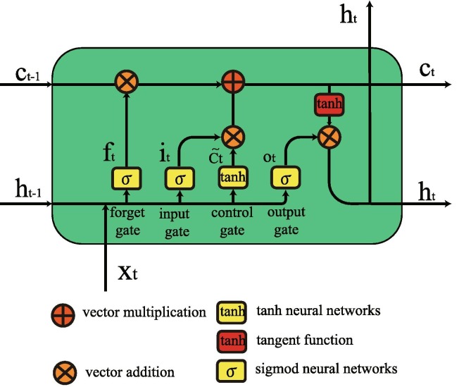
In 1997, Hochreiter and Schmidhuber [29] invented LSTM networks to deal with the long-term dependency problem. LSTM networks are well-suited to classifying, processing and making predictions based on time series data, since there can be lags of unknown duration between important events in a time series. LSTMs have the form of a chain of repeating modules, but the repeating module has a different structure. Instead of having a single neural network layer, there are four, interacting in a very special way (see Fig. 5 ). A common LSTM unit is composed of a memory cell, a forget gate, an input gate and an output gate, where the forget gate’s purpose is to selectively forget the information in the cell state, the input gate decides what new information is stored in the cell state, and the output gate decides what value we desire to output. The cell remembers values over arbitrary time intervals and the three gates regulate the flow of information into and out of the cell. The structure of LSTM is drawn in Fig. 6 . In the diagram, each line carries an entire vector, from the output of one node to the input of others. The circles represent pointwise operations, and the yellow boxes are learned neural network layers.
Fig. 5.
LSTM architecture contains four interacting layers.
Fig. 6.
LSTM cell architecture.
Gates in LSTM assist in information processing by using an activation sigmoid function, and the output is either 0 or 1. “0” means the gates are blocking everything, and “1” means gates are allowing everything to pass through it. The equations for the gates in LSTM are
| (1) |
where represent forget gate, input gate and output gate, respectively. represents the sigmoid function, is relevant weight in respective gate x associated with each LSTM block, is the previous output at timestamp denotes the current input vector at timestamp t, and is bias neurons at gate x. The equations for the cell state, candidate cell state and the final output are
| (2) |
where and represent the new and previous cell states (memory) at timestamps t and , respectively. refers to a tanh output and represents candidate for cell state at timestamp t, and represents the element wise multiplication of the vectors.
XGBoost
A scalable machine learning system for tree boosting is called as extreme gradient boosting algorithm (XGBoost), which is an optimized distributed gradient boosting library and can efficiently examine the importance of all input features. It has demonstrated to be a reliable and efficient machine learning problem solver [30], [31]. Compared with other gradient boosting algorithms, XGBoost can gather a strong classifier from a set of weak classifiers and display the following advantages: (1) effectively handle missing values; (2) be able to prevent overfitting; (3) parallel and distributed calculation reduce running time. The purpose of XGBoost is to employ a gradient descent optimization methodology and arbitrary differentiable loss functions to minimize the loss function by adding weak learners, i.e., to define and optimize the objective function. XGBoost attempts to minimize the regularized objective as follows:
| (3) |
where L is the training loss function that measures the deviation between the value predicted by our model and the actual value . is the regularization function that measures the complexity of the model, which tends to prevent overfitting. f is a function in the functional space , and is the set of all possible regression trees. In order to minimize the objective function, XGBoost uses parameters to find an optimal tree structure employing a greedy search algorithm.
Evaluation parameters
We evaluate the predictive effect of our model using four popular forecasting parameters such as: Mean Absolute Error (MAE), Mean Square Error (MSE), Root Mean Square Error (RMSE), and Mean Absolute Percentage Error (MAPE), as follows:
| (4) |
| (5) |
| (6) |
| (7) |
where n is the number of observations, and is the error between the forecasted value and actual value. MAE is an arithmetic average of the absolute errors between the prediction and true value, which gives the mean of the absolute forecasting error. MSE is a loss function to measure the error between predict value and true value. RMSE is a frequently used measure of the differences between values predicted by a model or an estimator and the values observed. It is the square root of the average squared error. MAPE quantifies accuracy as a percentage which can be calculated as a cumulative absolute percent error for each time frame, as the actual values minus the predicted values divided over the actual values. That is, it depicts the mean error in percentage terms.
Materials
Time series prediction is a method to forecast upcoming trends of the given historical dataset with temporal features. If input data has temporal components, the prediction of COVID-19 transmission will be effective. Statistical properties such as mean, variance and standard deviation also change with respect to time.
The number of daily new confirmed COVID-19 cases in time series is collected from the World Health Organization website, see https://covid19.who. int. The data set is available in time series format with date, month, and year to ensure that the time component is not overlooked. In order to anticipate future diseases, our proposed models actively learn real-time data from current COVID-19 observations.
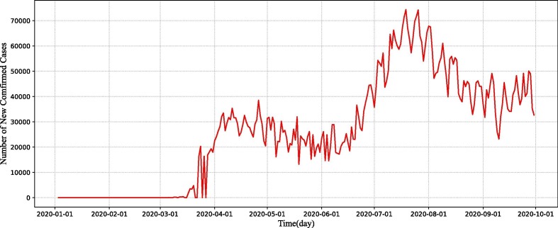
Fig. 7 illustrates the real trends from January 3, 2020 to September 30, 2020 in America. From the figure we can observe that, since mid-March, the number of confirmed cases has started to increase in the J-shaped trend. At that time, America has not yet implemented large-scale testing or isolation measures. The duration of infection persists for a long time, and there is a worse risk that infected individuals may be vulnerable to contact. From early April to the end of May, the number of daily new confirmed cases fluctuated within a certain range and did not begin to rise. Due to the implementation of large-scale testing measures and isolation of confirmed cases, the period of transmission has reduced in infected individuals. Owing to the adoption of stay-at-home orders and social distancing regulations, the chances of infected individuals encountering susceptible individuals have been limited, and the number of newly reported cases is no longer growing. However, from June to July, due to social events and other factors, the probability of human-to–human contact increased and the number of daily new confirmed cases resumed a sharp rise.
Fig. 7.
The number of daily new COVID-19 confirmed cases from January 3, 2020 to September 30, 2020 in America.
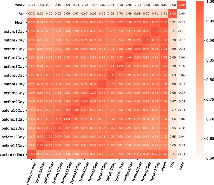
In time series analysis, we use historical data to create models and apply these models to predict the new outcome. From January to March 2020, America has not yet initiated large-scale research, isolation and treatment measures. Due to the fact that this part of time series data does not contain stable information, we intercept the data for new confirmed cases from April 1 to September 30 as modeling objects. Predicting the dynamics of transmission based on limited dataset is a challenging task. In order to find recent trends in infectious diseases, we separate the pre-processed data set into a training and test set and use the training data to train the LSTM and XGBoost models. Then, COVID-19 dataset is randomly split into 90% training set on which our models are trained and 10% testing set to test the performance of the model. Based on the investigation in Fig. 8 , we conduct a correlation test between daily new confirmed, mean and standard deviation of confirmed cases with human work week with an offset of (2 weeks before). It can be concluded that new diagnosed cases on that day has strongly positive correlation with the daily confirmed cases and mean of confirmed COVID-19 cases for the previous 14 days. The shorter the time interval, the stronger the association with the number of new confirmed individuals per day, meaning that the risk of new confirmed individuals being compromised by previously confirmed individuals is stronger.
Fig. 8.
The correlation heat map illustrates the relationship between daily new confirmed, mean, standard deviation of confirmed cases and human work week with an offset of ..
Experimental results analysis
The proposed model is developed with both LSTM and XGBoost that are conducted with open source libraries such as Numpy, Pandas and Keras.
Training
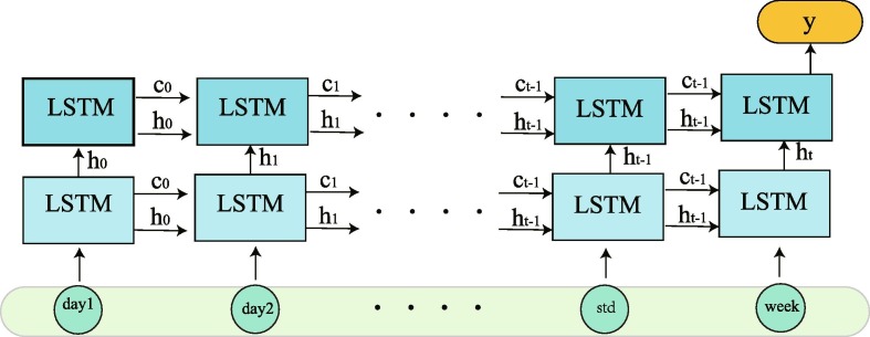
We use two-layers LSTM neural network structure to establish a model, which is shown in Fig. 9 .
Fig. 9.
Double layers LSTM network structure.
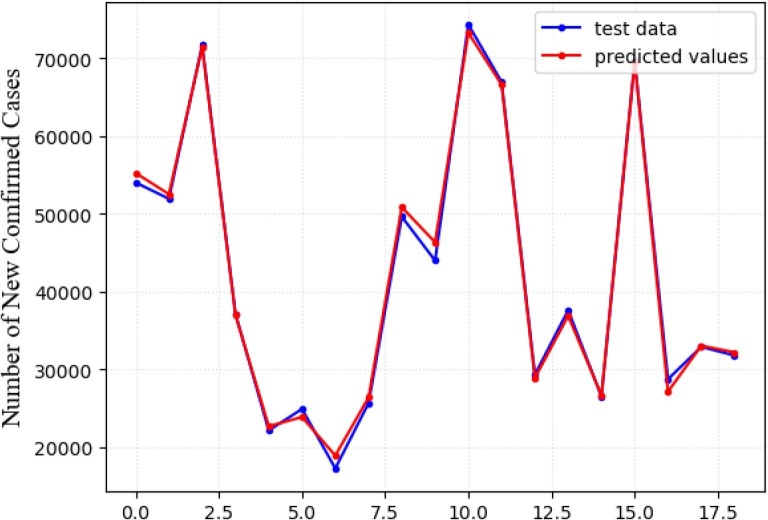
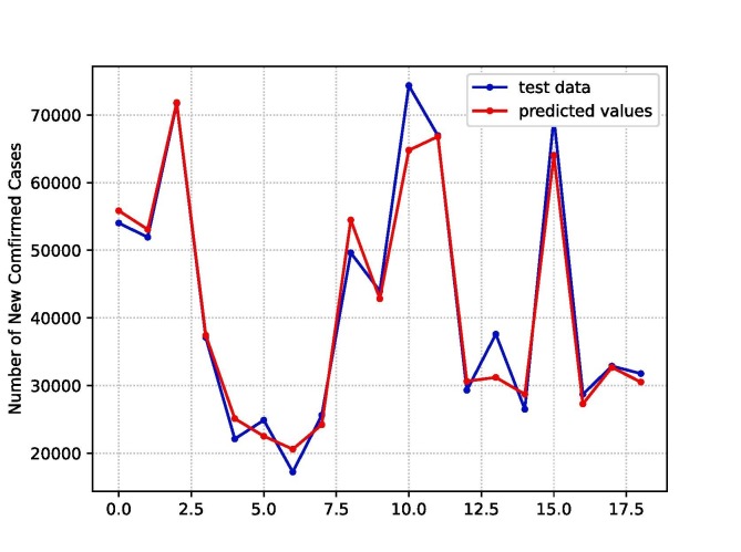
LSTM model differs from statistical models in several respects, for example, the proposed LSTM network matches real-time data and without any assumptions when choosing hyperparameters. In our LSTM model, we train and test the network on the currently available America dataset. Fig. 10 represents the simulation of LSTM model with reasonable parameter features which provides a good match to the data on infected COVID-19 cases in America from April 1, 2020 to September 30, 2020.
Fig. 10.
Prediction of the LSTM model on test set (red line). The blue line represents the actual values of test set.
Fitting with the training sample, the XGBoost model is used to estimate the number of new confirmed cases in the test set. The prediction result is shown in Fig. 11 , the blue curve shows the actual time series data and the red curve represents the prediction using XGBoost. From Fig. 10, Fig. 11, it can be concluded that LSTM prediction produce better result than XGBoost.
Fig. 11.
Prediction of the XGBoost model on test set (red line). The blue line represents the actual values of test set.
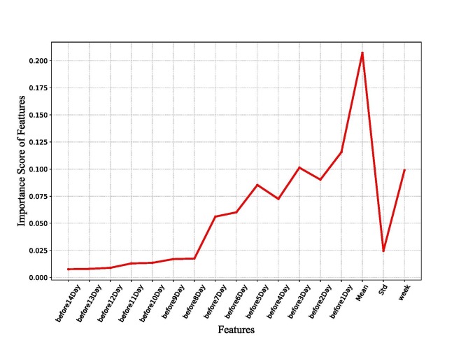
In order to determine the contribution of features of the XGBoost model, a graph is drawn after determining the significance score of each feature of the model (see Fig. 12 ). From Fig. 12, the most important feature is the mean, followed by the number of daily new confirmed cases over the previous 7 days. In other words, there is a high correlation between the number of new cases of the day and the number of new infections per day over the previous few days. In addition, the day of the week has a high contribution rate to the model. This indicates that the number of new confirmed cases of the day is closely related to whether it is a working day. Therefore, communication in the workplace is a critical way to spread the disease of COVID-19. In areas with serious epidemics, steps are required to avoid working to obstruct the route of disease transmission.
Fig. 12.
Features importance base on XGBoost.
We summarize the four values of MAE, MSE, RMSE and MAPE in Table 1 . Comparing the four evaluation parameters of LSTM and XGBoost models, it can be observed that LSTM performs better in terms of accuracy among two machine learning models. LSTM has the smaller and . XGBoost shows how much each feature contributed to the final forecast, and the interpretability of the model is greater than that of the LSTM.
Table 1.
Parameters evaluation for the LSTM and XGBoost model.
| Models | MAE | MSE | RMSE | MAPE(%) |
|---|---|---|---|---|
| LSTM | 771 | 962577 | 981 | 2.32 |
| XGBoost | 2658 | 11964681 | 3459 | 7.21 |
Prediction
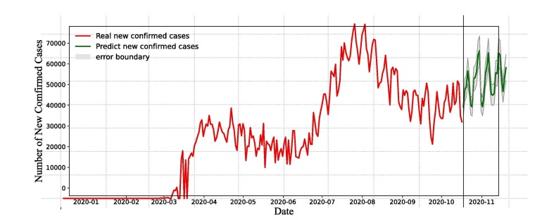
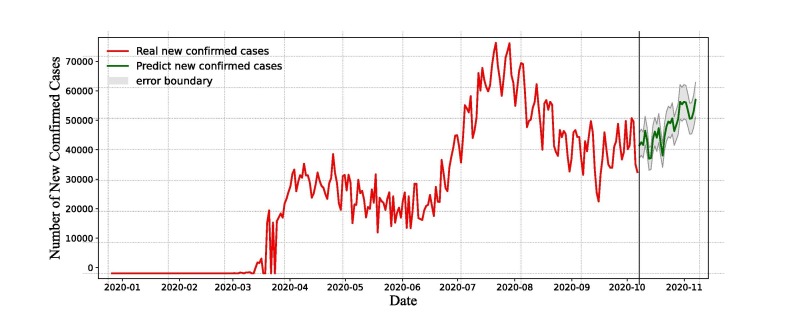
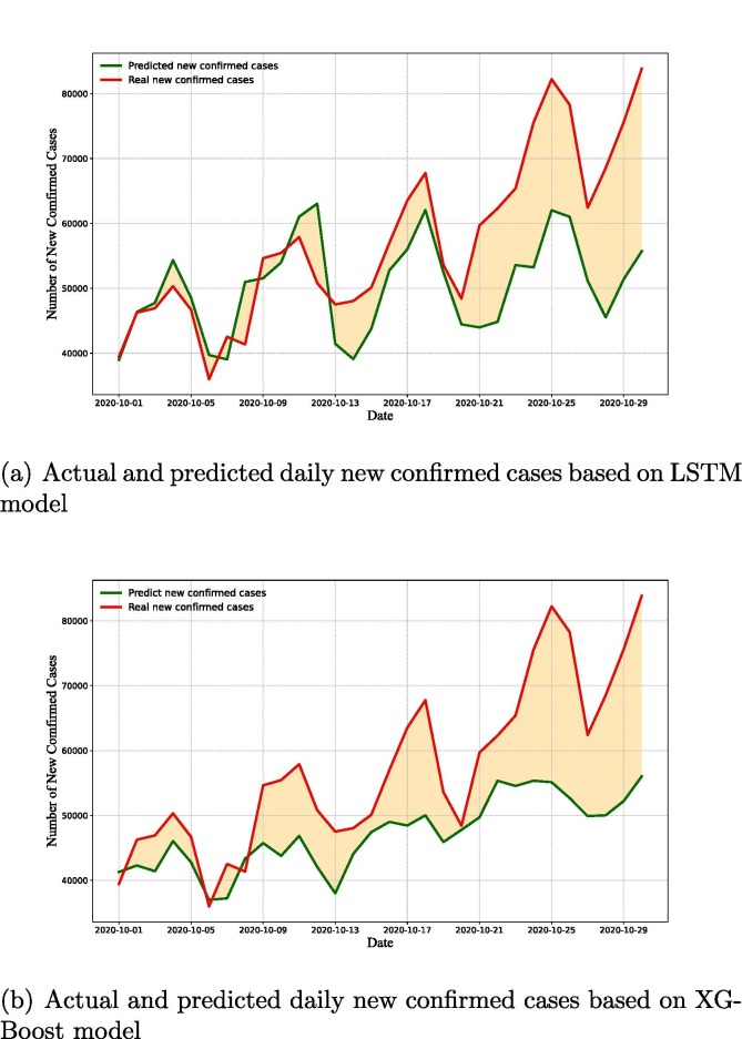
Based on assumptions (A1)-(A3), the number of new confirmed cases is determined by the disease transmission force and the investment in disease prevention resources. The time series data provide existing information on the disease spread and the management of investment resources, and these informations can assess the recent daily new confirmed cases. According to the assumptions, applying the feature set by the current time series data, we employ LSTM and XGBoost models to fit COVID-19 cases from April 1, 2020 to September 30, 2020, and report a 30-day forecast of the COVID-19 pandemic. Fig. 13, Fig. 14 represent time series actual and forecasted data of America using LSTM and XGBoost models, respectively. Actual (solid red line) and forecasted (solid green line) data can be visualize graphically in Fig. 13, Fig. 14.
Fig. 13.
The prediction results of LSTM model. The error bound is calculated based on MAPE.
Fig. 14.
The prediction results of XGBoost model. The error bound is calculated based on MAPE.
Fig. 13 indicates that the number of daily new confirmed cases fluctuates between and for the next 30 days, and the data will fluctuate over a certain period. It can be shown that the number of daily new confirmed cases maintains high level. From Fig. 14, XGBoost forecasts that the number of daily new confirmed cases will fluctuate frequently and not vanish in the next month. Daily new confirmed cases can be estimated to remain over 30, 000 and a downward trend is not occurring, with current disease prevention measures, the social environment and investment in medical services unchanged. The spread of the disease will not be fully prevented by current prevention, control measures and medical services.
The 30-day forecast of the new confirmed cases as a function of time (i.e., number of days) is shown in Fig. 15 . The reported cases were represented by red line, the LSTM and XGBoost model’s forecasts were represented by green color lines. The 30-day ahead forecast follows a periodic growth (as per LSTM model, see Fig. 15(a)) and an upward trend (as per XGBoost model, see Fig. 15(b)) in the number of daily new confirmed cases in America. The expected number of daily new confirmed cases was predicted to be between to on October 2020 which was not very close to the actual value, but LSTM prediction (see Fig. 15) is higher than the XGBoost prediction (see Fig. 15(b)). Because the actual data grows rapidly in a short period of time, other factors (e.g., social events, state elections) must be considered along with daily cases in order to appropriately estimate the real scenario.
Fig. 15.
Actual new confirmed cases (red line) vs. 30-day ahead forecast of daily new confirmed cases (green line).
Conclusion and discussion
COVID-19 is spreading at an astonishing speed, threatening both human life and the economy. Because of the rising magnitude of COVID-19 cases, the function of machine learning is critical in the current context. The approach of employing machine learning for time-series prediction, particularly in COVID-19, was effective in modeling and predicting the virus spreading end status.
In this study, we introduce a machine learning based on the LSTM and XGBoost models to investigate the future trend of COVID-19 in America and evaluate the important features based on the reported COVID-19 cases. To train and test the models used for our study, we use data up to September 30, 2020. The models utilized in this work are also based on data-driven approaches, and we examine our models predictions using MAE, MSE, RMSE and MAPE. We wished to analyze and compare the capability of LSTM and XGBoost models to interpret the complex trend in time series, and verify our four assumptions that presented at that time period by measuring our results, and finally, forecasting new cases of the next 30 days. Our approaches and forecast outcomes will assist in limiting COVID-19 pandemic infections.
We put out four assumptions (A1)-(A4) based on the analysis of the medical community’s research on the transmitting properties of COVID-19 disease. By using LSTM and XGBoost machine learning algorithms to model the time series data of daily new confirmed COVID-19 cases in America, these methods play a vital role in the analysis and prediction of disease trend scenarios. The results of test set show that MAPE of the LSTM and XGBoost algorithms reach and , respectively. It is also evident from Fig. 10, Fig. 11 that our LSTM model has the lower metrics value. In addition, the models project that the country has a tentative range between 30,000 to 70,000 new cases by October illustrated in Fig. 13, Fig. 14. Based on the aforementioned evidences and problems, we obtain that: (1) the period of infection with COVID-19 disease in an infected person lasts less than 14 days; (2) workplace is an essential way of spreading the COVID-19 disease, and suspension of work in serious outbreak areas is a critical control measure; (3) the number of new confirmed cases in America will fluctuate in range of 30,000 to 70,000 and remain at a high level.
In the absence of a broadly available COVID-19 vaccination, the effect of preventing strategies such as maintaining social distancing, wearing masks and lockdown suggests that the transmission of infectious disease can be greatly decreased by certain preventive measures. Prediction of future COVID-19 cases will be useful for government authorities, researchers and planners to administer facilities and coordinate medical resources in the near future. It is therefore possible for other nations to adopt the suggested frameworks and prevention measures.
There are several limitations to our proposed models. For one thing, the sample dimension is relatively small and should be expanded if the model is to be generalized. For another thing, different smoothing models can be utilized to achieve a better fitting curve and consequently a better forecast. And thirdly, the impact of the change of the degree of public cooperation, government policies and the stochastic factors are not taken into account in our model.
Declaration of Competing Interest
The authors declare that they have no known competing financial interests or personal relationships that could have appeared to influence the work reported in this paper.
Acknowledgements
This research is partially supported by Qing Lan Project of Jiangsu Province, the National Natural Science Foundation of China (No. 11601226, 71871115), Postgraduate Research & Practice Innovation Program of Jiangsu Province (No. KYCX21_1070).
References
- 1.Yang C.Y., Wang J. A mathematical model for the novel coronavirus epidemic in Wuhan, China. Math Biosci Eng. 2020;17(3):2708–2724. doi: 10.3934/mbe.2020148. [DOI] [PMC free article] [PubMed] [Google Scholar]
- 2.Alkahtani B.S.T., Alzaid S.S. A novel mathematics model of COVID-19 with fractional derivative stability and numerical analysis. Chaos, Solitons Fractals. 2020;138 doi: 10.1016/j.chaos.2020.110006. [DOI] [PMC free article] [PubMed] [Google Scholar]
- 3.Adekola H.A., Adekunle I.A., Egberongbe H.O., Onitilo S.A., Abdullahi I.N. Mathematical modeling for infectious viral disease: the COVID-19 perspective. J Public Affairs. 2020;20(4) doi: 10.1002/pa.2306. [DOI] [PMC free article] [PubMed] [Google Scholar]
- 4.Jiang F.Y., Zhao Z.F., Shao X.F. Time series analysis of COVID-19 infection curve: a change-point perspective. J Econometrics. 2020 doi: 10.1016/j.jeconom.2020.07.039. [DOI] [PMC free article] [PubMed] [Google Scholar]
- 5.Arora P., Kumar H., Panigrahi B.K. Prediction and analysis of COVID-19 positive cases using deep learning models: a descriptive case study of India. Chaos, Solitons Fractals. 2020;139 doi: 10.1016/j.chaos.2020.110017. [DOI] [PMC free article] [PubMed] [Google Scholar]
- 6.Kírbaş İ., Sőzen A., Tuncer A.D., ş Kazancíoğlu F. Comparative analysis and forecasting of COVID-19 cases in various European countries with ARIMA, NARNN and LSTM approaches. Chaos, Solitons Fractals. 2020;138 doi: 10.1016/j.chaos.2020.110015. [DOI] [PMC free article] [PubMed] [Google Scholar]
- 7.Alballa N., Al-Turaiki I. Machine learning approaches in COVID-19 diagnosis, mortality, and severity risk prediction: a review. Inform Med Unlocked. 2021;24 doi: 10.1016/j.imu.2021.100564. [DOI] [PMC free article] [PubMed] [Google Scholar]
- 8.Chimmula V.K.R., Zhang L. Time series forecasting of COVID-19 transmission in Canada using LSTM networks. Chaos, Solitons Fractals. 2020;135 doi: 10.1016/j.chaos.2020.109864. [DOI] [PMC free article] [PubMed] [Google Scholar]
- 9.Tomar A., Gupta N. Prediction for the spread of COVID-19 in India and effectiveness of preventive measures. Sci Total Environ. 2020;728 doi: 10.1016/j.scitotenv.2020.138762. [DOI] [PMC free article] [PubMed] [Google Scholar]
- 10.Wang P.P., Zheng X.Q., Ai G., Liu D.Y., Zhu B.R. Time series prediction for the epidemic trends of COVID-19 using the improved LSTM deep learning method: case studies in Russia, Peru and Iran. Chaos, Solitons Fractals. 2020;140 doi: 10.1016/j.chaos.2020.110214. [DOI] [PMC free article] [PubMed] [Google Scholar]
- 11.Dastider A.G., Sadik F., Fattah S.A. An integrated autoencoder-based hybrid CNN-LSTM model for COVID-19 severity prediction from lung ultrasound. Comput Biol Med. 2021;132:104296. doi: 10.1016/j.compbiomed.2021.104296. [DOI] [PMC free article] [PubMed] [Google Scholar]
- 12.Gautam Y. Transfer learning for COVID-19 cases and deaths forecast using LSTM network. ISA Trans. 2021 doi: 10.1016/j.isatra.2020.12.057. [DOI] [PMC free article] [PubMed] [Google Scholar]
- 13.Vaid A., Somani S., Russak A.J., De Freitas J.K., Chaudhry F.F. Machine learning to predict mortality and critical events in a cohort of patients with COVID-19 in new york city: model development and validation. J Med Internet Res. 2020;22(11) doi: 10.2196/24018. [DOI] [PMC free article] [PubMed] [Google Scholar]
- 14.Wang K., Zuo P.Y., Liu Y.W., Zhang M., Zhao X.F., Xie S.P., Zhang H., Chen X.L., Liu C.Y. Clinical and laboratory predictors of in-hospital mortality in patients with coronavirus disease-2019: a cohort study in Wuhan, China. Clinical Infectious Diseases. 2020;71(16):2079–2208. doi: 10.1093/cid/ciaa538. [DOI] [PMC free article] [PubMed] [Google Scholar]
- 15.Rechtman E., Curtin P., Navarro E., Nirenberg S., Horton M.K. Vital signs assessed in initial clinical encounters predict COVID-19 mortality in an NYC hospital system. Sci Rep. 2020;10:21545. doi: 10.1038/s41598-020-78392-1. [DOI] [PMC free article] [PubMed] [Google Scholar]
- 16.Yan L., Zhang H.T., Goncalves J., Xiao Y., Wang M.L., Guo Y.Q. A mechine learning-based model for survivial prediction in patients with severe COVID-19 infection. Health Sci. 2020 doi: 10.1101/2020.02.27.20028027. [DOI] [Google Scholar]
- 17.Li W.T., Ma J., Shende N., Castaneda G., Chakladar J., Tsai J.C., Apostol L., Honda C.O., Xu J., Wong L.M., Zhang T., Lee A., Gnanasekar A., Honda T.K., Kuo S.Z., Yu M.A., Chang E.Y., Rajasekaran M.R., Ongkeko W.M. Using machine learning of clinical data to diagnose COVID-19: a systematic review and meta-analysis. BMC Med Inform Decis Mak. 2020;20:247. doi: 10.1186/s12911-020-01266-z. [DOI] [PMC free article] [PubMed] [Google Scholar]
- 18.Katrakazas C., Michelaraki E., Sekadakis M., Ziakopoulos A., Kontaxi A. Identifying the impact of the COVID-19 pandemic on driving behavior using naturalistic driving data and time series forecasting. J Safety Res. 2021 doi: 10.1016/j.jsr.2021.04.007. [DOI] [PMC free article] [PubMed] [Google Scholar]
- 19.Kukar M., Gunc̆ar G., Vovko T., Podnar S., C̆ernelc̆ P., Brvar M. COVID-19 diagnosis by routine blood tests using machine learning. Sci Rep. 2021;11:10738. doi: 10.1038/s41598-021-90265-9. [DOI] [PMC free article] [PubMed] [Google Scholar]
- 20.Chan J.F.W., Yuan S.F., Kok K.H., To K.K.W. A familial cluster of pneumonia associated with the 2019 novel coronavirus indicating person-to-person transmission: a study of a family cluster. The Lancet. 2020;395(10223):514–523. doi: 10.1016/S0140-6736(20)30154-9. [DOI] [PMC free article] [PubMed] [Google Scholar]
- 21.Lai C.C., Shih T.P., Ko W.C., Tang H.J., Hsueh P.R. Severe acute respiratory syndrome coronavirus 2 (SARS-CoV-2) and coronavirus disease-2019 (COVID-19): the epidemic and the challenges. Int J Antimicrob Agents. 2020;55(3) doi: 10.1016/j.ijantimicag.2020.105924. [DOI] [PMC free article] [PubMed] [Google Scholar]
- 22.Wang D.W., Hu B., Hu C., Zhu F.F., Liu X., Zhang J., Wang B.B., Xiang H., Cheng Z.S., Xiong Y., Zhao Y., Li Y.R., Wang X.H., Peng Z.Y. Clinical characteristics of 138 hospitalized patients with 2019 novel coronavirus infected pneumonia in Wuhan, China. J Am Med Assoc. 2020;323(11):1061–1069. doi: 10.1001/jama.2020.1585. [DOI] [PMC free article] [PubMed] [Google Scholar]
- 23.Anderson R.M., Heesterbeek H., Klinkenberg D., Hollingsworth T.D. How will country-based mitigation measures influence the course of the COVID-19 epidemic? The Lancet. 2020;395(10228):931–934. doi: 10.1016/S0140-6736(20)30567-5. [DOI] [PMC free article] [PubMed] [Google Scholar]
- 24.Jin Y.H., Cai L., Cheng Z.S., Cheng H., Deng T., Fan Y.P. A rapid advice guideline for the diagnosis and treatment of 2019 novel coronavirus (2019-nCoV) infected pneumonia (standard version) Military Med Res. 2020;7(1):4. doi: 10.1186/s40779-020-0233-6. [DOI] [PMC free article] [PubMed] [Google Scholar]
- 25.Li Q., Guan X.H., Wu P., Wang X.Y., Zhou L., Tong Y.Q., Ren R.Q., Leung K.S.M., Lau E.H.Y., Wong J.Y., Xing X.S., Xiang N.J., Wu Y., Li C., Chen Q., Li D., Liu T., Zhao J., Liu M., Tu W.X., Chen C.D., Jin L.M., Yang R., Wang Q., Zhou S.H., Wang R., Liu H., Luo Y.B., Liu Y., Shao G., Li H., Tao Z.F., Yang Y., Deng Z.Q., Liu B.X., Ma Z.T., Zhang Y.P., Shi G.Q., Lam T.T.Y., Wu J.T., Gao G.F., Cowling B.J., Yang B., Leung G.M., Feng Z.J. Early transmission dynamics in Wuhan, China, of novel coronavirus–infected pneumonia. New England J Med. 2020;382(13):1199–1207. doi: 10.1056/NEJMoa2001316. [DOI] [PMC free article] [PubMed] [Google Scholar]
- 26.Guan W.J., Ni Z.Y., Hu Y., Liang W.H., Ou C.Q., He J.X., Liu L., Shan H., Lei C.L., Hui D.S.C., Du B., Li L.J., Zeng G., Yuen K.Y., Chen R.C., Tang C.L., Wang T., Chen P.Y., Xiang J., Li S.Y., Wang J.L., Liang Z.J., Peng Y.X., Wei L., Liu Y., Hu Y.H., Peng P., Wang J.M., Liu J.Y., Chen Z., Li G., Zheng Z.J., Qiu S.Q., Luo J., Ye C.J., Zhu S.Y., Zhong N.S. Clinical characteristics of coronavirus disease 2019 in China. New England J Med. 2020;382(18):1708–1720. doi: 10.1056/NEJMoa2002032. [DOI] [PMC free article] [PubMed] [Google Scholar]
- 27.Lauer S.A., Grantz K.H., Bi Q.F., Jones F.K., Zheng Q.L., Meredith H.R., Azman A.S., Reich N.G., Lessler J. The incubation period of coronavirus disease 2019 (COVID-19) from publicly reported confirmed cases: estimation and application. Ann Intern Med. 2020;172(9):577–582. doi: 10.7326/M20-0504. [DOI] [PMC free article] [PubMed] [Google Scholar]
- 28.Zhang X.S., Vynncky E., Charlett A., De Angelis D., Chen Z.J., Liu W. Transmission dynamics and control measures of COVID-19 outbreak in China: a modelling study. Sci Rep. 2021;11:2652. doi: 10.1038/s41598-021-81985-z. [DOI] [PMC free article] [PubMed] [Google Scholar]
- 29.Hochreiter S., Schmidhuber J. Long short-term memory. Neural Comput. 1997;9(8):1735–1780. doi: 10.1162/neco.1997.9.8.1735. [DOI] [PubMed] [Google Scholar]
- 30.Zheng Y.C., Zhu Y.H., Ji M.Q., Wang R.P., Liu X.F., Zhang M.D., Liu J., Zhang X.C., Qin C.H., Fang L., Ma S.H. A learning-based model to evaluate hospitalization priority in COVID-19 pandemics. Patterns. 2020;1(6) doi: 10.1016/j.patter.2020.100092. [DOI] [PMC free article] [PubMed] [Google Scholar]
- 31.Hu C.A., Chen C.M., Fang Y.C., Liang S.J., Wang H.C., Fang W.F., Sheu C.C., Perng W.C., Yang K.Y., Kao K.C., Wu C.L., Tsai C.S., Lin M.Y., Chao W.C. Using a machine learning approach to predict mortality in critically ill influenza patients: a cross-sectional retrospective multicentre study in Taiwan. BMJ Open. 2020;10(2) doi: 10.1136/bmjopen-2019-033898. [DOI] [PMC free article] [PubMed] [Google Scholar]


