Changes in spatial organization following an acute epizootic: Tasmanian devils and their transmissible cancer

Abstract

Epidemiological studies commonly monitor host population density but rarely account for how transmission dynamics might be influenced by changes in spatial and social organization that arise from high mortality altering population demography. Devil facial tumour disease (DFTD), a novel transmissible cancer, caused almost 100% mortality of its single host, the Tasmanian devil, and a >90% local population decline since its emergence 20 years ago. We compare size and overlap in home ranges in a devil population before and 15 years after disease outbreak. We used location data collected with VHF tracking collars in 2001 and GPS collars in the same area in 2015 and 2016. Density of adult devils, calculated from live trapping data in the same years, show a strong decrease following the disease outbreak. The decline in density was accompanied by a reduction in female home range size, a trend not observed for males. Both spatially explicit population modelling and animal tracking showed a decrease in female home range overlap following the DFTD outbreak. These changes in spatial organisation of the host population have the potential to alter the local transmission dynamic of the tumours. Our results are consistent with the general theory of sex-biased spatial organization mediated by resource availability and highlight the importance of incorporating spatial ecology into epidemiological studies.

1. Introduction

Acute disease outbreaks can decrease the density of their hosts, and in so doing can alter the spatial and social structure of the host population. Classic epidemiological models use temporal changes in host density to predict disease transmission (De Castro and Bolker, 2005; Cooch et al., 2012). A pathogen with a density-dependent transmission can die out when the host population declines below the threshold required to maintain the epidemic (Deredec and Courchamp, 2003). Pathogens with frequency-dependent transmission, on the other hand, lack this threshold and can, in theory, drive the host population to extinction (McCallum, 2012). Yet, if mortality is high, population decline can be rapid with consequent changes in per-capita resource availability. If resources are homogenously distributed in the landscape, inter-individual competition should lead to higher spatial segregation (Kjellander et al., 2004) resulting in an interconnected host population at a lower density. In this context, the transmission of a disease may be locally reduced due to lower contact rate between hosts but may still be able to spread through the whole population (Sanchez and Hudgens, 2015). However, in the presence of a heterogeneous resource distribution, remnant individuals will most likely concentrate their activity within the areas of higher resources (Newsome et al., 2013). Locally, the host density may remain high, providing suitable ground to sustain a disease transmission. But, in the broader landscape, a patchy spatial distribution could challenge the spread of the disease between patches (Manlove et al., 2014). These often-neglected ecological feedbacks could influence ongoing disease transmission dynamics and the long-term evolution of host-pathogen systems.

Since its discovery in 1996, the Tasmanian devil facial tumour disease (DFTD), a host-specific transmissible cancer with an almost 100% mortality rate within 12 months after first clinical signs, has resulted in sustained local population declines of up to 90% (McCallum et al., 2007). In less than twenty years, the spread of the disease resulted in the endemic Tasmanian devil (Sarcophilus harrisii) listed as endangered by the IUCN (Hawkins et al., 2008). Transmission occurs via transfer of live tumour cells, which necessitate direct contact between individuals with injurious biting behaviour. Inter-individual interactions occur all year round but peak during the mating season in February–March (Hamilton et al., 2019). The strong link between transmission and the annual mating season (Hamede et al., 2008) means that DFTD has a strong component of frequency-dependent transmission. Yet, more than twenty years after the DFTD outbreak, no local extinctions have been reported and devils are still present, albeit at very low densities, even in long diseased areas (Lazenby et al., 2018). A consequence of the sexually related transmission route is the quasi absence of tumour infection in juvenile devils allowing for annual recruitment. But at low density, diseased populations present a much reduce age structure with a high proportion of juveniles (less than 2 years old) and a few mature individuals rarely older than 2 years old and presenting facial tumours (Lachish et al., 2009). In comparison, Tasmanian devils in healthy populations can live up to 6 years. The dispersal usually take place during the first year of life between December and February. Naturally biased towards longer dispersal for males, this pattern was accentuated following the outbreak of DFTD by a reduction in dispersal distances for females but not for males (Lachish et al., 2011). Research has focussed on the epidemiology (McCallum et al., 2009; Hamede et al., 2015; Wells et al., 2017) and potential evolutionary response of devils (Epstein et al., 2016; Wright et al., 2017; Hubert et al., 2018; Margres et al., 2018), with the potential effects of the disease on the spatial organization of the host populations not investigated.

The spatial organization of a species is classically defined by the size and overlap of individual home ranges (Arden-Clarke, 1986; Belcher and Darrant, 2004; Fattebert et al., 2016). While most ecologists agree on the concept of home range given by Burt (1943), there is no universally accepted method to quantify and represent home range (Worton, 1987; Walter et al., 2015). For decades, home ranges have been calculated using individual movements recorded by telemetry (Harris et al., 1990; Cagnacci et al., 2010), a rapidly evolving field due to advances in technology. While providing unprecedented knowledge of animal behaviour, the most recent estimators of home range rely on high-resolution tracking data using global positioning system (GPS) that are often not available with historical data, which is typically based on very high frequency (VHF) radiotracking. Tracking data using VHF provide a lower frequency of location fixes with a lower precision than those using GPS (Hebblewhite and Haydon, 2010). Yet, the much lower cost of VHF technology and the smaller size of the trackers makes it still a valuable choice for wildlife ecologists (Jerosch et al., 2017).

Like many carnivore species (Sandell, 1989), devils are solitary animals (Guiler, 1970), yet, two studies conducted in healthy populations are in general concordance of devils having overlapping and therefore non-defended home ranges. In a study in the early 1980s, long before DFTD emerged, Pemberton (1990) used radiocollars to describe spatial patterns in one population in northeast Tasmania (wukalina/Mt William National Park). This site is a mixture of intact natural vegetation and regenerating pasture and had a high devil population (a minimum of 140 individuals caught with 50 traps over 25 km² and ten days). Home range size was estimated at 13.3 km² (n = 9, range: 4–26.7, method: minimum convex polygon, MCP 100%) with no differences between males and females. The home ranges presented a highly overlapping distribution (84.1%) defined as the proportion of a home range shared by any other individual. In that study, only 2–3 radiocollars were used sequentially on devils for short periods of time (3–22 days).

More recently, Andersen et al. (2017) deployed GPS tracking collars on 18 devils (2012 and 2013) in a population on the west coast of Tasmania in the last area remaining free of the disease. This area is a mix of forest and coastal scrub in the Arthur Pieman Conservation Area and an adjacent livestock property with forest fragmented by pasture. Home ranges were estimated at 18.1 km² for males (n = 8, range: 10.2–25.7, method: movement-based kernel density estimator, MKDE 95%) and 11.6 km² for females (n = 10, range: 8.4–16.3, method: MKDE 95%). In this study, the average overlap of home ranges was 41% (G. Andersen, personal communication).

The challenge for conservation biologists is to compare data from recent GPS tracking with data collected during past VHF studies. While the technology differs, VHF and GPS tracking data do provide comparable estimations of home range size, given similar sampling effort (Pellerin et al., 2008). This has been demonstrated in studies of either the same individuals (whitetailed deer; Fieberg and Kochanny (2005)) or simultaneously on different individuals in the same population (wild turkeys; Niedzielski and Bowman (2016) and American alligator; Skupien et al. (2016)). These studies relied on long-term low frequency VHF tracking to complement the fine-scale GPS data. Alternatively, Pellerin et al. (2008) show that tracking data recorded with VHF and GPS from the same animal at the same time (roe deer) provide comparable estimations of home range sizes if sampling effort is similar. This study used the kernel density estimator (KDE) and a fixed smoothing parameter that provides a better estimation of home ranges than the more simplistic minimum convex polygon (MCP) often used with low quality VHF data.

In this study, we present the first tracking data of a diseased population of Tasmanian devils. We use location data of Tasmanian devils collected in the same area before (VHF) and fifteen years after (GPS) the outbreak of DFTD. After accounting for sampling heterogeneity (frequency, number of locations and tracking duration) between the technologies, we assess the impact of the decline in population density on the size and overlap of the home ranges. Tasmanian devil being solitary animals we expect males and females to present a different response in spatial organisation due to different ecological and social needs. We discuss the potential implication of our results for disease transmission.

2. Materials and methods

We conducted our study on Freycinet Peninsula (42°03′53”S, 148°17′14”E, Fig. 1), a topographically varied and rugged landscape on the East Coast of Tasmania, Australia (Lachish et al., 2007). The west side, along the moulting lagoon (a large and shallow salt water body), is flat and open, balanced between pasture and native grassland. Most of this area consists of private bush blocks with a low human density. The eastern half features a topographically varied and rugged landscape on a mixture of sandstone with large granite boulders mostly covered by dry eucalypt forests encompassing small patches of wet forest (mainly at the bottom of steep gullies). Most of this area is protected under the Freycinet National Park and the Coles Bay Conservation Area. The study area is limited to the south by the Hazards, an abrupt mountain range (450 m) closing the narrowest part of the peninsula. The average monthly temperature range between 9 and 18 °C, with an annual average rainfall of 690 mm.

Fig. 1.

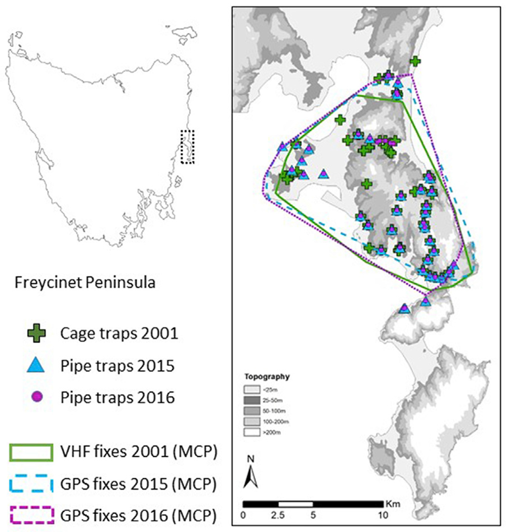
Location of the study area (Freycinet peninsula) and sampling design. Green crosses represent the locations of the 60 cage traps set in 2001 and used for the density estimates (secr). The blue triangles and the purple dots represent the location of the PVC pipes traps used in 2015 (n = 43) and 2016 (n = 49). The three lines represent the 100% minimum convex polygons (MCP) encompassing all tracking locations. Green line shows the MCP of 2001 based on VHF collars. Blue and purple lines represent the MCP from the GPS tracking of 2015 and 2016 respectively. The grey-scaled background shows the elevation on the peninsula. (For interpretation of the references to colour in this figure legend, the reader is referred to the Web version of this article.)

The 100 km² area was part of a long-term study aimed at monitoring the devil population and DFTD epidemic dynamics (Jones et al., 2019). Part of this monitoring included live trapping of devils during the Austral winter (June–July) with individual identification of each animal (ear tattoos <2004; microchips >2003) and determination of their sex and age (Table 1). The presence of visual signs of DFTD and the reproductive status of all females (visual observation of the pouch) were recorded. Due to the difficulty of access, the trap locations were not homogeneously distributed over the area but followed roads and accessible four-wheel drive tracks. The study area has been monitored with 60 cage traps in 2001 (mean distance = 449 m), 43 PVC pipe traps in 2015 (mean distance 626 m) and 49 PVC pipe traps in 2016 (mean distance = 556 m); 35 of the trap locations were identical in all three years (Fig. 1). The traps were checked in the morning after sunrise during seven contiguous nights. Both cage traps and pipe traps allowed for only one capture per night resulting in seven sampling occasion per trap location.

Table 1.

Winter trapping of Tasmanian devils on the Freycinet peninsula.

Year	Trap model	Number of traps	Male		Female
			Adult	Subadult	Adult	Subadult
2001	cage	60	18 (30)	9 (19)	21 (45)	17 (40)
2015	PVP pipe	43	5 (6)	10 (20)	3 (8)	7 (12)
2016	PVC pipe	49	5 (7)	6 (8)	6 (10)	6 (10)

Trapping data used to fit the spatially-explicit capture-recapture (secr) model. Sample size is given as the number of individual devil trapped with the number of captures in brackets. Each trap was set for seven contiguous nights in winter (June–July) with only one capture per night possible.

We used a spatially-explicit capture-recapture (secr) model (Efford et al., 2009) to estimate the winter population densities in the study area. We used a hazard half normal detection function and the Nelder and Mead (1965) maximization method of the likelihood. We followed Efford et al. (2016) by replacing σ (the spatial scale parameter of the secr models) in the detection function by a density (D) dependent parameter: k = σ D allowing us to calculate an index of home range overlap S₉₅ = 6σk². This index represents the number of individuals living within one 95% home range, i.e. a value of 1 (the minimum possible) indicates a solitary exclusive species, a value of 2 indicates exclusive pairs, more generally, the higher the index the more individuals overlap their activity within a population. Due to the shape of the study area, we used a spatial mask to restrict the density estimate to the emerged land mass and with a 9000 m buffer size around the trap locations. We allowed the density to vary per year (2001, 2015 and 2016) sex (female vs male) and age (adult vs subadult) by fitting a multisession model using the group function of the package secr v3.2.1. We also considered the possibility that devils may change their behaviour due to the presence of the traps (becoming trap shy or trap happy) by fitting a site and session specific learned response (function bk of the secr package) on the detection probabilities. Due to the limited sample size in 2015 and 2016 (Table 1), we could not include the group factors (sex or age) for the density dependent parameter k that was therefore modelled as year specific only (2001, 2015 and 2016). Density analyses were performed in R v3.6.1 (R Core Team, 2019).

During May 2001, before the DFTD outbreak, we fitted 42 VHF transmitters to male (n = 20) and female (n = 22) adult Tasmanian devils. Up to four daily radiolocations (one in late afternoon and three during night time) were attempted for each collar using four fixed towers and a mobile antenna mounted on a vehicle. We calculated the locations of the animals by triangulation using R v3.6.1 with the package sigloc v0.0.4 (Lenth, 1981). Due to the ruggedness and size of the study area, the signal from the VHF collars was often weak or bouncing, resulting in low success rate in animal location. Only animals with at least 15 location fixes were considered for this study (n = 19; 7 females and 12 males). At the time of the tracking, all females had small pouch young. In 2015 and 2016, respectively, 14 and 15 years after the disease outbreak, we deployed GPS collars in the same study area between August and December. Tracking data were available for 5 individuals in 2015 (3 females and 2 males) and 7 in 2016 (5 females and 2 males). Two females were fitted with a GPS collar in both 2015 and 2016 (Table 2). GPS location attempts were set hourly between 17:00 and 7:00 (i.e. night). All females equipped with a GPS collar had young in a den at the time of tracking. As none of the animals tracked for this study presented with clinical signs of DFTD, we were able to assess the impacts of the disease-driven population decline on individual home ranges, rather than on the direct pathological impact on the individual ranging behaviour.

Table 2.

Tasmanian devil tracking information and home range calculations.

Devil	Sex	Age (year)	Tracking data					Home rangea (km2)
			technology	Start	End	Days	Fixes	95%	50%
TD.039	f	3	VHF	3/05/2001	31/05/2001	28	21	34.2	7.1
TD.042	f	3	VHF	3/05/2001	29/05/2001	26	21	25.7	6.4
TD.058	f	5	VHF	10/05/2001	31/05/2001	21	19	41.9	9.5
TD.113	f	2	VHF	4/05/2001	28/05/2001	24	14	38.9	NA
TD.126	f	2	VHF	3/05/2001	31/05/2001	28	16	24.0	4.6
TD.134	f	2	VHF	6/05/2001	31/05/2001	25	20	27.2	4.7
TD.138	f	2	VHF	3/05/2001	31/05/2001	28	34	36.2	10.5
TD.003	m	5	VHF	2/05/2001	28/05/2001	26	19	16.1	NA
TD.015	m	3	VHF	4/05/2001	31/05/2001	27	23	20.0	3.7
TD.018	m	5	VHF	3/05/2001	31/05/2001	28	24	28.8	7.8
TD.026	m	3	VHF	2/05/2001	31/05/2001	29	29	30.2	4.3
TD.048	m	4	VHF	2/05/2001	30/05/2001	28	17	29.9	8.9
TD.053	m	4	VHF	6/05/2001	31/05/2001	25	43	36.3	7.9
TD.125	m	2	VHF	4/05/2001	31/05/2001	27	36	26.8	8.5
TD.153	m	2	VHF	5/05/2001	31/05/2001	26	39	41.2	9.9
TD.154	m	2	VHF	3/05/2001	31/05/2001	28	16	45.9	12.7
TD.158	m	2	VHF	3/05/2001	29/05/2001	26	43	38.9	10.4
TD.163	m	4	VHF	3/05/2001	24/05/2001	21	28	8.7	2.0
TD.188	m	2	VHF	3/05/2001	31/05/2001	28	28	41.9	10.1
TD.277	f	3	GPS	8/08/2015	7/09/2015	30	156	34.1	8.2
TD.522	f	4	GPS	13/08/2015	12/09/2015	30	216	13.0	3.3
TD.823	f	3	GPS	6/08/2015	5/09/2015	30	205	16.6	3.9
TD.085	m	3	GPS	12/08/2015	11/09/2015	30	207	26.9	6.8
TD.378	m	2	GPS	12/08/2015	11/09/2015	30	130	28.0	7.6
TD.455	f	2	GPS	3/09/2016	3/10/2016	30	260	17.3	4.3
TD.522	f	5	GPS	19/08/2016	18/09/2016	30	242	11.9	2.9
TD.625	f	2	GPS	3/09/2016	3/10/2016	30	201	40.7	8.9
TD.823	f	4	GPS	3/09/2016	3/10/2016	30	181	17.2	4.0
TD.979	f	2	GPS	25/08/2016	24/09/2016	30	230	13.8	3.1
TD.471	m	2	GPS	24/08/2016	23/09/2016	30	297	20.8	5.7
TD.554	m	2	GPS	1/09/2016	1/10/2016	30	262	29.2	7.2

^aFinal individual Home range size calculated with a Kernel Density Estimator (KDE) with a fix smoothing factor (h) of 500 m.

As the duration of the VHF tracking was shorter than the GPS tracking, we restricted the GPS data to the first 30 days of the tracking. The frequency of fixes within these 30-days periods was also lower and less regular for the VHF tracking (average of 26 locations, range: 16–43) than for the GPS tracking (average of 229 locations, range: 130–303). To account for this heterogeneous sampling effort, we first estimated an average (based on one hundred replicates) home range size (95% KDE) and core area (50% KDE) for increasing fractions of location fixes randomly selected from the tracking data (sequentially 10,15, 20, 25 and 40, but stopping before reaching the total number of location fixes available). We used a constant smoothing parameter (h) of 500 m, representing an averaged “href” value using bivariate normal KDE on individual tracking data using the total location fixes available over the 30-days period (Worton, 1989). We then fitted a logarithmic regression (Haines et al., 2009) on the sequential individual home range areas (including the maximum area estimated with the whole data set for all individuals followed by means of VHF telemetry). Following Odum and Kuenzler (1955), we considered the final home range sizes (95% and 50% KDE) as the first interval after which any additional location fix resulted in less than one percent increase of the predicted area (Fig. 2).

Fig. 2.

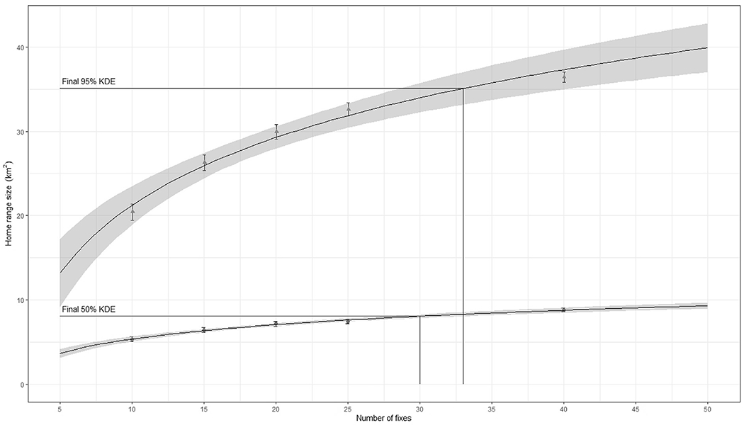
Estimation of the final home range size (95% kernel density estimator, KDE) and core area (50% KDE) for one female devil (TD.625) tracked with a GPS collar in 2016. Each triangle (95% KDE) and circle (50% KDE) represent the average size (y-axis) and 95% confidence interval of the home range based on 100 replicates of randomly selected location fixes from the tracking data (x-axis). The curves represent the logistic regressions fitted on the average sizes and the grey area the 95% confidence interval of the predicted regression. The final value for the home range and core area sizes correspond to the first interval of location fixes with an area increase of less than 1%.

To spatially represent the final home ranges (95% KDE), we first drew one hundred home ranges based on the repeated random selection of ten location fixes. Using a 50m× 50 m grid over the whole study area, we calculated the number of times each individual cell was included in the home ranges. The final shape of the home range was obtained by joining the cells according to their ranking, until the area of the shape matched the final area calculated on the curves. The analysis of home-range overlap was robust only for female devils, because of the low number of males tracked in 2015 and 2016. Each year, we measured the proportion of the home range overlap for each possible pair of females (Frey and Conover, 2007): Overlap AB = A∩B/A where A is the size of the home range of the first female and B the size of the home range of the second female. A∩B is the size of the area included in both home ranges. With this method, the overlap of the pair AB≠BA. Considering the low sample size, we used a Mann-Whitney-Wilcoxon test to compare the home range sizes (95% KDE and 50% KDE) and a Student’s t-test for the proportion of overlap between individuals before (2001) and after (2015–2016) the DFTD outbreak. All analyses were performed in R v3.6.1 using the packages adehabitatHR v0.4.16 (Calenge, 2006) and rgeos v0.5-2 (2019).

3. Results

Prior to the disease outbreak, the population structure of devils in the study area was balanced between males and females and between adults and subadults (Table 3). In 2015, devil densities were almost three times lower than before the outbreak of DFTD. Devil densities remained low in 2016. In all years, devils show a strong learned response to the traps with naive animals being three time more likely to be trapped than experienced individuals (i.e. after first trapping event). The overall decline in devil density following the DFTD epidemic was accompanied by a small reduction of the spatial scale parameter (k) and more apparent decrease in home range overlap index S₉₅ (Table 3), although for both parameters, the 95% confidence intervals overlapped. The data suggests that the decrease in density may have induced smaller home range sizes with a lower overlap at a population level.

Table 3.

Population densities of Tasmanian devils on the Freycinet Peninsula before the DFTD epidemic (2001)and 15 years after disease outbreak (2015 and 2016).

Year	Sex	Adults [n/km2]	Subadults [n/km2]	λ0 first capture	λ0 secondary captures	k	S95
2001	males	0.150 (0.100–0.223)	0.134 (0.088–0.204)	0.058 (0.042–0.081)	0.017 (0.006–0.045)	0.618 (0.514–0.744)	7.203 (4.974–10.432)
2001	females	0.160 (0.121–0.212)	0.155 (0.105–0.230)
2015	males	0.054 (0.032–0.091)	0.050 (0.030–0.084)	0.054 (0.032–0.091)	0.015 (0.005–0.046)	0.510 (0.376–0.692)	4.904 (2.662–9.033)
2015	females	0.057 (0.035–0.093)	0.056 (0.033–0.094)
2016	males	0.062 (0.040–0.097)	0.055 (0.041–0.100)	0.031 (0.025–0.037)	0.009 (0.003–0.024)	0.505 (0.440–0.579)	4.806 (3.654–6.321)
2016	females	0.066 (0.056–0.077)	0.064 (0.041–0.100)

Densities estimated using spatially explicit capture recapture model (secr). λ0 = cumulative hazard of detection; k = density dependent spatial scale factor; and S₉₅ = index of overlap in home range. Densities were modelled as sex (male vs female), age (adult vs subadult) and year (2001, 2015 and 2016) specific; λ0 varied per year and included a site-specific learned response, k and S₉₅ were dependent on year only. 95% confidence intervals for all values are indicated in brackets.

Following the decrease in population density, female 95% home ranges calculated with the tracking data were significantly smaller (Mann-Whitney-Wilcoxon test: w = 47, p = 0.029) (Fig. 3), with a similar trend for the 50% core areas (Mann-Whitney-Wilcoxon test: w = 8, p = 0.043). We found no apparent change in male home ranges and core areas (Mann-Whitney-Wilcoxon test: w = 32, p = 0.379 and w = 12, p = 0.226 respectively).

Fig. 3.

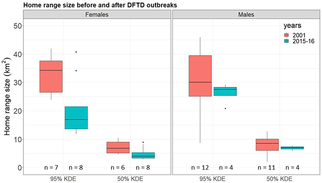
Distribution of home range (95% KDE) and core area (50% KDE) sizes for female and male devils before the DFTD outbreak (2001, red) and 15 years after DFTD arrival (2015–2016, blue). Sample sizes (n) are indicated above the x-axis. (For interpretation of the references to colour in this figure legend, the reader is referred to the Web version of this article.)

As devil density declined, female home range overlap (based on the tracking data) reduced from 40% in 2001 to 18% in 2015–2016 (Student’s t-test: t = −3.165, df = 44.779, p = 0.003), in line with the decrease of the S₉₅ estimates from the secr modelling (based on the trapping data). This decrease was stronger between females of the same age (3+ years old: from 63% to 17%; 2 years old: from 27% to 4%) than between older and younger females (2 years old ∩ 3+ years old: from 40% to 26%). This resulted in two spatially segregated pairs of females in 2016 (Fig. 4), TD.522 & TD.979 (red home ranges) in the west and TD.823 & TD.455 (blue home ranges) in the centre. Both pairs included one older female (3+ years old) and one younger female (2 years old). The home range of the last female (TD.625, purple home range) was further southeast but still overlapped slightly with the central pair.

Fig. 4.

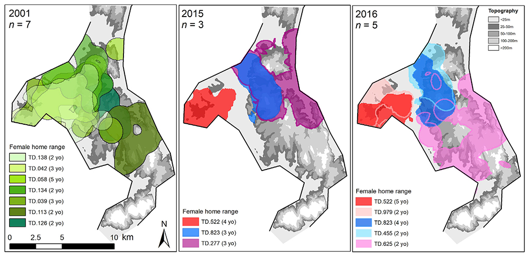
Spatial representation of female home ranges (95% KDE) before DFTD outbreak (2001) and 15 years after DFTD arrival (2015 and 2016). Two females (TD.522 and TD.823) were tracked both in 2015 and 2016. The black lines represent the coast and the grey scaled background shows the topography.

4. Discussion

Our results show that the DFTD outbreak in the Freycinet peninsula resulted in a strong decline in Tasmanian devil density. Based on two independent empirical data, we provide evidence of a change in the spatial organisation of the population. Female home range size and overlap decreased after the disease outbreak, a trend not observed for males. As DFTD transmission relies on direct contacts between individual hosts, the observed changed in spatial organisation may potentially alter the local epidemiology of the disease.

Several technical and biological factors constrain the sample size. First, the VHF tracking data provided a low success rate inherent to the technology at the time and the use of radio collars at large scale (100 km²) in rugged landscape, which we compensated for with repeated random resampling of all tracking data (VHF and GPS). Secondly, the tracking in 2001 and the tracking in 2015-16 took place at a different time of the year (May and September–October, respectively). This may have an effect on the movements of devils and could influence their home range size. Indeed, females in 2001 had very small young in the pouch while in 2015-16 females were caring for young in a den. In absence of yearlong tracking data for Tasmanian devils, it is difficult to quantify this seasonal effect. By avoiding the mating season (February–March) we have already removed a strong factor influencing home ranges. At the time of the GPS tracking, all females had dropped their young in the den (visual observation of the pouch while deploying the GPS collars) so they were more mobile than with large young in the pouch.

The small sample sizes in the two years post-DFTD outbreak limit the interpretability of our results, especially for the male home range overlap. This small sample size reflects the reality of working with a severely declined population of an endangered species. Our sample is as close to the true population as possible. Estimates of density based on the secr model indicate that we did track most of the adult females present in the study area, although males were underrepresented in our samples. In addition, the low capture rate in 2015 and 2016 prevented us to estimate sex and age specific spatial scale parameter (k) in the secr model. Given the observed stability of male’s home range size compared to female’s, the combination of both sexes could explain the lower decrease for the S₉₅ index of overlap from the secr model. Yet, because we used two methods on two independent datasets (trapping records and tracking data) to assess the changes in spatial organisation, we are confident in their ecological meaning. Our study highlights the challenge and importance of utilizing past data sets to understand current demographic and epidemiological patterns to improve the conservation of endangered species.

The rapid decrease in devil density caused by the DFTD epidemic likely resulted in an increase in per capita resources. Most of the study area being protected under the Freycinet National Park and the Coles Bay Conservation Area, no significant change in habitat occurred between the two study periods. There has been an increase in visitors in the last twenty years, but most of the tourism activity is concentrated around the town of Coles Bay (South of the study area) and mostly consist of diurnal activities. In absence of direct estimation of prey availability over the study area, we must rely on the relative stability of the habitat to consider a stable resource availability between 2001 and 2015–16. The observed changes in female home range size are therefore in accordance with the general theory that the spatial ecology of female mammals is driven by food resources and energetic requirements (Lawson Handley and Perrin, 2007; Said et al., 2009). Following an increase in per capita resources, females can reduce the energy and the time necessary to cover their own needs and to provision for their young, which generally result in smaller home range sizes (Sandell, 1989; Maletzke et al., 2014). In contrast, the spatial organization of males in solitary carnivores is driven by the opportunities for paternity success, which include the needs to maintain dominance (Clapham et al., 2012) and assess female reproductive status (Ramsey et al., 2002), two mechanisms reflected in our study by the higher stability in male home range sizes. In addition, an increase in precocial breeding has been documented following the spread of DFTD with subadults growing faster and becoming sexually active in their first year instead of their second year as commonly observed in healthy populations (Lachish et al., 2009). This is an additional support for an increase in per capita resources following DFTD outbreaks.

As most scavenging carnivores, devils display individual scrounging behaviour (i.e. exploiting resources discovered by others) leading to communal feeding (Pemberton and Renouf, 1993). While scrounging individuals may allow for higher densities for the same amount of resources (Coolen et al., 2007), their proportion in the population should decrease when resources become more abundant as individuals are more likely to find their own food than they are to benefit from conspecific foraging (Beauchamp, 2008). This is particularly relevant for Tasmanian devils that face risk of injuries due do aggressive behaviours when sharing large carrions (Pemberton and Renouf, 1993). Therefore, devils being mostly solitary and non-territorial, the increase in per capita resources following DFTD outbreak could potentially minimize conspecific tolerance and induce a stronger spatial segregation in populations (Gehrt and Fritzell, 1998). This supports the reduction of the home range overlap as measured by both the secr models (S₉₅ index) and the female home range overlap from the tracking data, two methods relying on independent empirical data (trapping and tracking).

The observed density-related changes in spatial organization would alter the network of social contact patterns between individuals in the population, with consequences for disease transmission. The reduced size and overlap between home ranges due to lower competition for food may result in a decrease in conflicts between individuals during the year (Sanchez and Hudgens, 2015). In addition, with the rapid decrease in density following DFTD outbreak, sexual selection could favour males investing more energy into single mating events and females becoming less selective in the choice of a partner (Lamb et al., 2017). Analyses of data collected using proximity-sensing radiocollars on two populations of devils at high density prior to DFTD outbreak showed that injurious biting events mostly occur during the mating season (Hamede et al., 2008) and directly relate to the number of partners, for both sexes (Hamilton et al., 2019). A reduction of the number of partners due to density related changes in spatial organisation could alter the spread of DFTD by limiting the direct transmission of the tumours within the population. Our findings suggests that changes in movement and spatial ecology have the potential to challenge the otherwise highly frequency-dependent transmission of DFTD (Sah et al., 2017). Building upon our study, additional tracking of Tasmanian devils should be conducted with three main questions. 1) What is the seasonal/annual pattern of movement and spatial organisation of Tasmanian devil (yearlong tracking of devils)? 2) Do tumours modify the movement behaviours of the infected host (tracking of DFTD infected animals)? 3) Does density driven change in spatial organisation directly induce a reduction in aggressive behaviours and injurious biting (simultaneous tracking of Tasmanian devils with GPS and proximity loggers)? A better understanding of the effect of DFTD on the spatial and movement ecology of its hosts will help understand the complex epidemiology of this rare disease and provide ground to refine the future management strategies for the emblematic Tasmanian devil.

5. Conclusion

Our study suggests changes in spatial organization of a host population following a rapid decrease in density induced by an acute epidemic outbreak. In accordance with the general theory of sex-biased spatial organization mediated by resource availability, we observed a reduction in female home range size and a lower home range overlap in the population. Because DFTD is mainly transmitted through direct injurious biting, the observed changes have the potential to alter the transmission of the disease by reducing the interactions between individuals. Further research is needed to better understand the interaction between density, spatial organisation and DFTD transmission to better manage the remnant wild populations of Tasmanian devils. Our findings highlight the importance of incorporating spatial ecology into epidemiological studies.

References

- Andersen GE, Johnson CN, Barmuta LA, Jones ME, 2017. Use of anthropogenic linear features by two medium-sized carnivores in reserved and agricultural landscapes. Sci. Rep 7,11624. [DOI] [PMC free article] [PubMed] [Google Scholar]
- Arden-Clarke CHG, 1986. Population density, home range size and spatial organization of the Cape clawless otter, Aonyx capensis, in a marine habitat. J. Zool 209, 201–211. [Google Scholar]
- Beauchamp G, 2008. A spatial model of producing and scrounging. Anim. Behav 76,1935–1942. [Google Scholar]
- Belcher CA, Darrant JP, 2004. Home range and spatial organization of the marsupial carnivore, Dasyurus maculatus maculatus (Marsupialia: dasyuridae) in south-eastern Australia. J. Zool 262, 271–280. [Google Scholar]
- Burt WH, 1943. Territoriality and home range concepts as applied to mammals. J. Mammal 24, 346–352. [Google Scholar]
- Cagnacci F, Boitani L, Powell RA, Boyce MS, 2010. Animal ecology meets GPS-based radiotelemetry: a perfect storm of opportunities and challenges. Phil. Trans. Biol. Sci 365, 2157–2162. [DOI] [PMC free article] [PubMed] [Google Scholar]
- Calenge C, 2006. The package “adehabitat” for the R software: a tool for the analysis of space and habitat use by animals. Ecol. Model 197, 516–519. [Google Scholar]
- Clapham M, Nevin OT, Ramsey AD, Rosell F, 2012. A hypothetico-deductive approach to assessing the social function of chemical signalling in a non-territorial solitary carnivore. PloS One 7, e35404. [DOI] [PMC free article] [PubMed] [Google Scholar]
- Cooch E, Conn P, Ellner S, Dobson A, Pollock K, 2012. Disease dynamics in wild populations: modeling and estimation: a review. J. Ornithol 152, 485–509. [Google Scholar]
- Coolen I, Giraldeau L-A, Vickery W, 2007. Scrounging behavior regulates population dynamics. Oikos 116, 533–539. [Google Scholar]
- De Castro F, Bolker B, 2005. Mechanisms of disease-induced extinction. Ecol. Lett 8, 117–126. [Google Scholar]
- Deredec A, Courchamp F, 2003. Extinction thresholds in host parasite dynamics. Ann. Zool. Fenn 40, 115–130. [Google Scholar]
- Efford MG, Borchers DL, Byrom AE, 2009. Density estimation by spatially explicit capture-recapture: likelihood-based methods. In: Thomson DL, Cooch EG, Conroy MJ (Eds.), Modeling Demographic Processes in Marked Populations. Springer US, Boston, MA, pp. 255–269. [Google Scholar]
- Efford MG, Dawson DK, Jhala YV, Qureshi Q, 2016. Density-dependent home-range size revealed by spatially explicit capture-recapture. Ecography 39, 676–688. [Google Scholar]
- Epstein B, Jones M, Hamede R, Hendricks S, McCallum H, Murchison EP, Schonfeld B, Wiench C, Hohenlohe P, Storfer A, 2016. Rapid evolutionary response to a transmissible cancer in Tasmanian devils. Nat. Commun 7, 12684. [DOI] [PMC free article] [PubMed] [Google Scholar]
- Fattebert J, Balme GA, Robinson HS, Dickerson T, Slotow R, Hunter LTB, 2016. Population recovery highlights spatial organization dynamics in adult leopards. J. Zool 299, 153–162. [Google Scholar]
- Fieberg J, Kochanny CO, 2005. Quantifying home-range overlap: the importance of the utilization distribution. J. Wildl. Manag 69, 1346–1359. [Google Scholar]
- Frey SN, Conover MR, 2007. Influence of population reduction on predator home range size and spatial overlap. J. Wildl. Manag 71, 303–309. [Google Scholar]
- Gehrt SD, Fritzell EK, 1998. Resource distribution, female home range dispersion and male spatial interactions: group structure in a solitary carnivore. Anim. Behav 55,1211–1227. [DOI] [PubMed] [Google Scholar]
- Guiler ER, 1970. Observations on the Tasmanian devil, Sarcophilus harrisii (Marsupialia:Dasyuridae): I. Numbers, home range, movements, and food in two populations. Aust. J. Zool 18, 49–62. [Google Scholar]
- Haines AM, Hernandez F, Henke SE, Bingham RL, 2009. A method for determining asymptotes of home-range area curves. In: Cederbaum S, Faircloth B, Terhune T, Thompson J, Carroll J (Eds.), Gamebird 2006: Quail VI and Perdix XII. 31 May - 4 June 2006. Warnell School of Forestry and Natural Resources, Athens, GA, USA, pp. 489–498. [Google Scholar]
- Hamede RK, McCallum H, Jones ME, 2008. Seasonal, demographic and density-related patterns of contact betweenTasmanian devils (Sarcophilus harrisii): implications for transmission of devil facial tumour disease. Austral Ecol. 33, 614–622. [Google Scholar]
- Hamede RK, Pearse AM, Swift K, Barmuta LA, Murchison EP, Jones ME, 2015. Transmissible cancer in Tasmanian devils: localized lineage replacement and host population response. In: Proceedings. Biological Sciences/the Royal Society, vol. 282. [DOI] [PMC free article] [PubMed] [Google Scholar]
- Hamilton DG, Jones ME, Cameron EZ, McCallum H, Storfer A, Hohenlohe PA, Hamede RK, 2019. Rate of intersexual interactions affects injury likelihood in Tasmanian devil contact networks. Behav. Ecol 30, 1087–1095. [Google Scholar]
- Harris S, Cresswell WJ, Forde PG, Trewhella WJ, Woollard T, Wray S, 1990. Home-range analysis using radio-tracking data–a review of problems and techniques particularly as applied to the study of mammals. Mamm Rev. 20, 97–123. [Google Scholar]
- Hawkins C, McCallum H, Mooney N, Jones M, Holdsworth M, 2008. Sarcophilus harrisii. The IUCN Red List of Threatened Species 2008 e.T40540A10331066.
- Hebblewhite M, Haydon DT, 2010. Distinguishing technology from biology: a critical review of the use of GPS telemetry data in ecology. Phil. Trans. Biol. Sci 365, 2303–2312. [DOI] [PMC free article] [PubMed] [Google Scholar]
- Hubert J-N, Zerjal T, Hospital F, 2018. Cancer- and behavior-related genes are targeted by selection in the Tasmanian devil (Sarcophilus harrisii). PloS One 13, e0201838. [DOI] [PMC free article] [PubMed] [Google Scholar]
- Jerosch S, Gotz M, Roth M, 2017. Spatial organisation of European wildcats (Felis silvestris silvestris) in an agriculturally dominated landscape in Central Europe. Mamm. Biol 82, 8–16. [Google Scholar]
- Jones M, Hamede R, Storfer A, Hohenlohe P, Murchison EP, McCallum H, 2019. Tasmanian devil facial tumour disease: ecology and evolution of an uncommon enemy. In: Wilson K, Fenton A, Tompkins DM (Eds.), Wildlife Disease Ecology: Linking Theory to Data and Application. Cambridge University Press. [Google Scholar]
- Kjellander P, Hewison AJM, Liberg O, Angibault JM, Bideau E, Cargnelutti B, 2004. Experimental evidence for density-dependence of home-range size in roe deer (Capreolus capreolus L.): a comparison of two long-term studies. Oecologia 139, 478–485. [DOI] [PubMed] [Google Scholar]
- Lachish S, Jones ME, McCallum H, 2007. The impact of disease on the survival and population growth rate of the Tasmanian devil. J. Anim. Ecol 76, 926–936. [DOI] [PubMed] [Google Scholar]
- Lachish S, McCallum H, Jones ME, 2009. Demography, disease and the devil: life-history changes in a disease-affected population of Tasmanian devils (Sarcophilus harrisii). J. Anim. Ecol 78, 427–436. [DOI] [PubMed] [Google Scholar]
- Lachish S, Miller KJ, Storfer A, Goldizen AW, Jones ME, 2011. Evidence that disease-induced population decline changes genetic structure and alters dispersal patterns in the Tasmanian devil. Heredity 106, 172–182. [DOI] [PMC free article] [PubMed] [Google Scholar]
- Lamb CT, Mowat G, Gilbert SL, McLellan BN, Nielsen SE, Boutin S, 2017. Density-dependent signaling: an alternative hypothesis on the function of chemical signaling in a non-territorial solitary carnivore. PloS One 12, e0184176. [DOI] [PMC free article] [PubMed] [Google Scholar]
- Lawson Handley LJ, Perrin N, 2007. Advances in our understanding of mammalian sex-biased dispersal. Mol. Ecol 16, 1559–1578. [DOI] [PubMed] [Google Scholar]
- Lazenby BT, Tobler MW, Brown WE, Hawkins CE, Hocking GJ, Hume F, Huxtable S, Iles P, Jones ME, Lawrence C, Thalmann S, Wise P, Williams H, Fox S, Pemberton D, 2018. Density trends and demographic signals uncover the long-term impact of transmissible cancer in Tasmanian devils. J. Appl. Ecol n/a-n/a. [DOI] [PMC free article] [PubMed] [Google Scholar]
- Lenth RV, 1981. On finding the source of a signal. Technometrics 23,149–154. [Google Scholar]
- Maletzke BT, Wielgus R, Koehler GM, Swanson M, Cooley H, Alldredge JR, 2014. Effects of hunting on cougar spatial organization. Ecol. Evol 4, 2178–2185. [DOI] [PMC free article] [PubMed] [Google Scholar]
- Manlove KR, Cassirer EF, Cross PC, Plowright RK, Hudson PJ, 2014. Costs and benefits of group living with disease: a case study of pneumonia in bighorn lambs (Ovis canadensis). Proc. Biol. Sci 281, 20142331–20142331. [DOI] [PMC free article] [PubMed] [Google Scholar]
- Margres MJ,Jones M, Epstein B, Kerlin DH, Comte S, Fox S, Fraik AK, Hendricks SA, Huxtable S, Lachish S, Lazenby B, O’Rourke SM, Stahlke AR, Wiench CG, Hamede R, Schönfeld B, McCallum H, Miller MR, Hohenlohe PA, Storfer A, 2018. Large-effect loci affect survival in Tasmanian devils (Sarcophilus harrisii) infected with a transmissible cancer. Mol. Ecol [DOI] [PMC free article] [PubMed] [Google Scholar]
- McCallum H, 2012. Disease and the dynamics of extinction. Phil. Trans. Roy. Soc. Lond. B Biol. Sci 367, 2828–2839. [DOI] [PMC free article] [PubMed] [Google Scholar]
- McCallum H, Jones ME, Hawkins C, Hamede RK, Lachish S, Sinn DL, Beeton N, Lazenby B, 2009. Transmission dynamics of Tasmanian devil facial tumor disease may lead to disease-induced extinction. Ecology 90, 3379–3392. [DOI] [PubMed] [Google Scholar]
- McCallum H, Tompkins DM, Jones ME, Lachish S, Marvanek S, Lazenby B, Hocking G, Wiersma J, Hawkins CE, 2007. Distribution and impacts of Tasmanian devil facial tumor disease. EcoHealth 4, 318–325. [Google Scholar]
- Nelder JA, Mead R, 1965. A simplex method for function minimization. Comput. J 7, 308–313. [Google Scholar]
- Newsome TM, Ballard GA, Dickman CR, Fleming PJS, van de Ven R, 2013. Home range, activity and sociality of a top predator, the dingo: a test of the Resource Dispersion Hypothesis. Ecography 36, 914–925. [Google Scholar]
- Niedzielski B, Bowman J, 2016. Home range and habitat selection of the female eastern wild Turkey at its northern range edge. Wildl. Biol 22, 55–63. [Google Scholar]
- Odum EP, Kuenzler EJ, 1955. Measurement of territory and home range size in birds. Auk 72, 128–137. [Google Scholar]
- Pellerin M, Saïd S, Gaillard J-M, 2008. Roe deer Capreolus capreolus home-range sizes estimated from VHF and GPS data. Wildl. Biol 14,101–110. [Google Scholar]
- Pemberton D, 1990. Social Organisation and Behaviour of the Tasmanian Devil, Sarcophilus harrisii. Science Faculty, Zoology Department. University of Tasmania, p. 272. [Google Scholar]
- Pemberton D, Renouf D, 1993. A field-study of communication and social-behavior of the tasmanian devil at feeding sites. Aust. J. Zool 41, 507–526. [Google Scholar]
- R Core Team, 2019. R: A Language and Environment for Statistical Computing. R Foundation for Statistical Computing, Vienna, Austria. [Google Scholar]
- Ramsey D, Spencer N, Caley P, Efford M, Hansen K, Lam M, Cooper D, 2002. The effects of reducing population density on contact rates between brushtail possums: implications for transmission of bovine tuberculosis. J. Appl. Ecol 39, 806–818. [Google Scholar]
- Sah P, Leu ST, Cross PC, Hudson PJ, Bansal S, 2017. Unraveling the disease consequences and mechanisms of modular structure in animal social networks. Proc. Natl. Acad. Sci. Unit. States Am [DOI] [PMC free article] [PubMed] [Google Scholar]
- Saïd S, Gaillard J-M, Widmer O, Débias F, Bourgoin G, Delorme D, Roux C, 2009. What shapes intra-specific variation in home range size? A case study of female roe deer. Oikos 118, 1299–1306. [Google Scholar]
- Sanchez JN, Hudgens BR, 2015. Interactions between density, home range behaviors, and contact rates in the Channel Island fox (Urocyon littoralis). Ecol. Evol 5, 2466–247 . [DOI] [PMC free article] [PubMed] [Google Scholar]
- Sandell M, 1989. The mating tactics and spacing patterns of solitary carnivores. In: Gittleman JL (Ed.), Carnivore Behavior, Ecology, and Evolution. Springer US, Boston, MA, pp. 164–182. [Google Scholar]
- Skupien GM, Andrews KM, Norton TM, 2016. Benefits and biases of VHF and GPS telemetry: a case study of American alligator spatial ecology. Wildl. Soc. Bull 40, 772–780. [Google Scholar]
- Walter W, Onorato D, Fischer J, 2015. Is there a single best estimator? Selection of home range estimators using area-under-the-curve. Mov. Ecol 3,1–11. [DOI] [PMC free article] [PubMed] [Google Scholar]
- Wells K, Hamede RK, Kerlin DH, Storfer A, Hohenlohe PA, Jones ME, McCallum HI, 2017. Infection of the fittest: devil facial tumour disease has greatest effect on individuals with highest reproductive output. Ecol. Lett 20, 770–778. [DOI] [PMC free article] [PubMed] [Google Scholar]
- Worton BJ, 1987. A review of models of home range for animal movement. Ecol. Model 38, 277–298. [Google Scholar]
- Worton BJ, 1989. Kernel methods for estimating the utilization distribution in home-range studies. Ecology 70,164–168. [Google Scholar]
- Wright B, Willet CE, Hamede R, Jones M, Belov K, Wade CM, 2017. Variants in the host genome may inhibit tumour growth in devil facial tumours: evidence from genome-wide association. Sci. Rep 7, 423. [DOI] [PMC free article] [PubMed] [Google Scholar]