Effects of quarantine disobedience and mobility restrictions on COVID-19 pandemic waves in dynamical networks

Abstract

For the global COVID-19 pandemic it is still not adequately understood how quarantine disobedience and change in mobility restrictions influence the pandemic spreading and waves. Here, we propose a new metapopulation epidemiological model as a network composed of equal clusters to predict the course of the epidemic based on the contiguous spreading between the neighbours, the probability of quarantine misbehaviour, and the probability of mobility, which control contacts outside the cluster. We exemplify the model by comparing simulation results with real data on COVID-19 pandemic in Croatia. Fitting the data over the first and second pandemic waves, when the probability of mobility is set by the stringency index, the probability of quarantine misbehaviour is found by a Bayesian optimization yielding a fascinating agreement between the daily COVID-19 deaths and model output and efficiently predicting the timing of pandemic bursts. A sudden increase in the probability of quarantine misbehaviour alongside the sudden increase in the probability of mobility generate the model third wave in good agreement with daily COVID-19 deaths.

In the history of mankind infectious diseases have killed more people than all the wars together [1] making them the major cause of deaths. Over only a few years in the 14th century, the plague killed up to 200 million people in Europe and North Africa, while after the First World War the Spanish flu caused up to 100 million deaths worldwide. Nowadays the world is faced again with a new pandemic, called COVID-19, which has drawn the attention of so many scientists as probably neither of the previous diseases in human history [2], [3], [4], [5], [6], [7], [8]. Managing the scale of pandemics and understanding their spreading mechanism in social communities is a key world topic due to the immersive impact of pandemics on human society, public health, and global economy.

The spread and mortality of infectious diseases depends on many factors where the robustness of the healthcare system [9] and the patterns of how people contact each other are among the most salient. The knowledge of social mobility patterns helps the public health workers identify and isolate individuals who have been in contact with the diseased and therefore prevent the spots of potential outbreaks.

To control the COVID-19 spread, practically all countries have carried out varying healthcare policies such as school and border closures, social distancing, self-isolation, wearing masks in public [10], where some countries have decided to enforce complete lock-downs in order to prevent the virus to spread freely and exponentially [11] that may lead to highly undesirable overburdening of the healthcare system when it becomes totally inefficient. The measures intended to avoid this catastrophic scenario are commonly known as flattening the curve [12].

However, while measures imposed by governments serve to prevent the ongoing spread of the virus and mitigate the potential catastrophe on both the healthcare system and the entire economy, once the data on the disease start to accumulate, for varying policies and measures the mathematical models serve to improve the effectiveness of intervention strategies in slowing the spread; offering reliable predictions about the number of infected, total deaths, or the number of people that need to be vaccinated to create herd immunity. During the last decades the seminal work of Kermack and McKendrick and their SIR model based on ordinary differential equations (ODE) has been largely applied to mimic the spread of infectious diseases [13]. To take into account heterogeneity in mixing patterns commonly observed in populations, network epidemic models have been heavily employed [14], [15], [16], [17], [18], [19], [20], [21], [22], [23], [24] to investigate sequential partnership patterns [25], concurrency in relationships [25], and the impact of various social biases on the spread of epidemics [19], [23], as with many other diseases.

A large number of papers combine traditional stochastic, and SIR epidemic models with complex systems approaches in order to properly explain COVID-19 spreading. Analysing epidemiological data from China, Chinazzi et al. [26] apply a global metapopulation disease transmission model combining a metapopulation network approach with real-world data to conclude that early detection, hand washing, self-isolation, and household quarantine are more effective in mitigating the pandemic than travel restrictions. Based on a novel epidemic spreading model, Zlatic et al. [27] report a bi-stable phase behavior and demonstrate that before the pandemic enters into the giant phase, an early testing procedure in COVID-19 crisis may keep it under control, where even a very small change in the rate of testing can increase or decrease the size of the whole epidemic for various orders of magnitude. Chang et al. [28] introduce a metapopulation SEIR model to simulate the spread of SARS-CoV-2. They analyse cell phone data in 10 of the largest US metropolitan areas and create fine-grained, dynamic mobility networks. By capturing who is infected at which locations the proposed model can inform more effective and equitable policy responses to COVID-19. Chande et al. [29] analyse the effects of large events, indoor gatherings and mask-wearing to the disease spreading. The main goal of this study is to help individuals and public authorities in making decisions.

Some studies focus on the robustness of public health systems. In a study focused on the capacity of hospitals and healthcare system [30], the authors propose an approach for modeling the number of COVID-19 and non-COVID-19 patients that may use ICU capacity. The authors estimate the ICU capacity for non-COVID-19 patients. Cinelli et al. [31] focus on a side effect of the COVID-19 epidemic i.e. an infodemic of true and false news. The authors try to fit the information diffusion with epidemic spreading models characterizing the basic reproduction number.

Here, applying a new epidemic spreading dynamical network model on pandemic data from Croatia, we demonstrate that the model exhibits a striking agreement with empirical results in predicting the outbreaks timing during the pandemic. Out of 18 parameters in the model, only 2 are free, while the rest are fixed to comply with empirical findings. To illustrate how misbehaviour and change in mobility policy affect pandemics, applying Bayesian optimization we demonstrate that once the first and the second pandemic waves are over a sudden increase in the probability of quarantine misbehaviour together with the sudden increase of the probability of mobility yield the model third pandemic wave in good agreement with daily COVID-19 deaths registered in Croatia.

1. Model

The COVID-19 pandemic evolved in sequences of pandemic waves where periods of low and high fractions of diseased repeatedly replace each other. We model this ability of a pandemic to spontaneously recover using a complex networks framework. Specifically, the model is based on a dynamical network characterised by stochastic contiguous spreading where each node can fail (i) independently of other nodes, (ii) contiguously due to failures of neighboring nodes, but also (iii) spontaneously recover after an inactive period of time [32], [33]. These networks are shown to exhibit phase-flipping between two collective network modes, “active” and “inactive” [32].

We define a network composed of $M$ equal, but mutually unlinked clusters of size $k$. Each cluster is a fully connected network and represents the fundamental societal unit whose individuals are constantly in contact (household, family, close neighbours etc.). The model assumes that the population mixes homogeneously (some extensions in this regard where also explored, see risky group behavioural scenario), i.e. it is equally likely that the disease can be transmitted between any two subjects, regardless of their age, gender, and place where they live, at home or at work.

• (i)At each time $t$, each subject (node) can independently get diseased with COVID-19, with a very small probability $q$. This infection, independent of the surrounding, we assign as the node $i$’s internal infectious state denoted by spin $|s_i〉$. In reality this kind of infection models individuals who got infected outside the network (i.e. people who travel from a country to another) and it is how the pandemic begins.
• (ii)Due to contiguous spreading, every diseased node may affect any other individual in its surrounding. Precisely we define that every infected neighbour of a healthy node $i$ has a probability $r$ of transmitting the disease, if infection occurs the node becomes externally diseased which state is denoted by spin $|S_i〉$. Node $i$—described by the two-spin state $|s_i,S_i〉$—is active only if all spins are up, i.e, $|s_i,S_i〉=|1,1〉$.
• (iii)An individual recovers or dies from COVID-19 after a time $\tau$ since failure.
• (iv)To account for mobility restrictions, we assume that at each time step, each node is randomly chosen with a probability of mobility $p_1$ to establish a contact with what we call, the central unit, representing work, school, shopping place etc. In the central unit, each subject has a chance to get COVID-19 infected with probability $\widehat{r}$.
• (v)To account for the level of disobedience among the individuals of the society, we assume that among contacts of COVID-19 diseased nodes, there is the probability $p_2$ of not following a quarantine restriction or self-isolation. Thus, $p_2$ measures the probability of quarantine misbehaviour or disobedience.

Different assumptions (iii)–(v) were also considered where the recovery time $\tau$, the probabilities $p_1$ and $p_2$ and the clusters size $k$ are not constant but rather come from a distribution (normal or exponential), leading to similar results.

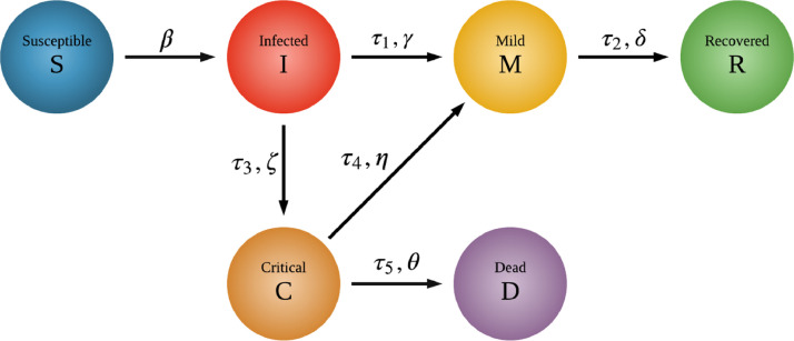
The stochastic infection model considers six stages of COVID-19 disease progression: susceptible individuals (S), infected with SARS-CoV-2, where the infected persons are not aware that they have the disease, but still transmit it to others (I), symptomatic infection with mild symptoms (M), infection with severe COVID-19 symptoms (C), recovery with immunity (R) and COVID-19 deaths (D). A stochastic process non related to COVID-19 with a single internal spin $|s_i〉$ was also added, its two stages being: unspecified critical severe disease (U) and non-COVID-19 deaths (N). Stages C and U represent the intensive care unit (ICU) patients.

1.1. Transition probabilities between different stages

Fig. 1 identifies six different COVID-19 stages quantified by their transition probabilities ($\beta$, $\gamma$, $\delta$, $\eta$, $\zeta$, $\theta$), where only two are free. Parameters related to both COVID-19 and unspecified respiratory diseases we obtain from worldwide medical sources [34], [35], [36], [37], [38], [39], [40], [41], [42], [43], [44], [45]. $\beta$ depends on the network structure, internal and external failures and the transmission probability $r$ which according to recent studies [35] is in the range $2.6\%-17.4\%$; $\delta =1$ and the rest of the six COVID-19 transition parameters have only two degrees of freedom:

Fig. 1.

Diagram of the epidemic model states. The six stages of COVID-19 disease progression and their transition probabilities: susceptible (S), infected (I), mild (M), critical (C), recovered with immunity (R) and died from COVID-19 (D). Infected asymptomatic stage (I) describes the situation when the individual is already contagious, but does not show any symptoms. Besides these states the model differentiates between COVID-19 and non-COVID-19 related critical state and death.

I $\underrightarrow{\zeta }$ C: A small fraction of those who develop symptoms begin to develop more serious conditions. Based on data from more than 13 countries, the European Centre for Disease Prevention and Control [36] (ECDPC) estimates that around $42\%$ of confirmed cases are hospitalised and $2\%-7\%$ are hospitalized in ICU. Similarly, other studies report that the rate of ICU admission among hospitalized patients with COVID-19 varies from $3\%$ to $100\%$ of admitted patients [37].

C $\underrightarrow{\theta }$ D: Studies showed that the mortality among intensive care patients with COVID-19 was very high and ranged from $1\%$ to $86\%$ of admitted patients [37]

The median time for onset of symptoms is $5-6$ days [38] (${\tau }_1$ and ${\tau }_3$), the median time from onset to clinical recovery for mild cases is approximately 2 weeks [38] (${\tau }_2$) and for patients with severe or critical disease is more than 3 weeks [38] (${\tau }_4+{\tau }_2$). The time of stay in ICU (which results in death or recovery) is 2–12 days [39] (${\tau }_4$ and ${\tau }_5$).

1.2. Population

Our model allows to define arbitrarily many categories (types) of individuals and their ratios in the network. We modelled the entire population as two age groups, whose difference is a different probability of disease survival. The total population in the simulations is of $N={10}^6$ actors.

1.3. Physical distancing strategies

Physical distancing strategies and social contact-reduction policies between the meta-population $k$-units, we model using an additional stochastic process implemented on the network model. At each step, each individual has the probability $p$ to establish a contact with the central unit: $p=p_1$ for those individuals which have no sick (M or C) individuals in their fundamental unit and $p=p_1·p_2$ if there is at least one sick individual. For a susceptible (S) individual, the probability of becoming infected while in the central unit is

$$\widehat{r}=\kappa ·r·\frac{b}{n},$$ (1)

where $n$ represents the total number of individuals in the central unit, $b$ represents the total number of infected individuals in the central unit, $r$ is the probability of external infection, see (ii), and $\kappa$ is a free parameter representing the density of the population (in our simulations fixed as $\kappa =2.5$ whose simulated $R_0$ yielded best agreement with existing sources [40] for COVID-19). We simulated two behavioral scenarios :

• 1.Households/basic - The only individuals who are assumed to go to the central unit are susceptible (S), infected (I) and recovered (R). Individuals in symptomatic mild (M) or critical (C or U) node state are assumed not to go to the central unit ($p_1=0$); either they are sick and conscientious enough not to spread the disease, or they are ICU patients.
• 2.Special/risky groups - A fraction of the individuals will go to the central unit less frequently. For these the probabilities are $p_1/10$ and $p_2/10$, where $p_1$ and $p_2$ are the parameters for the rest of the population. These individuals are assumed to be in the more risky category, i.e. older than 60 years, (the remaining individuals behave as in 1.).

2. Simulations and results

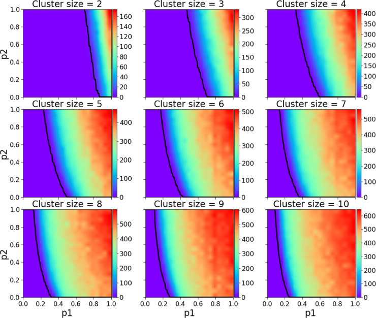
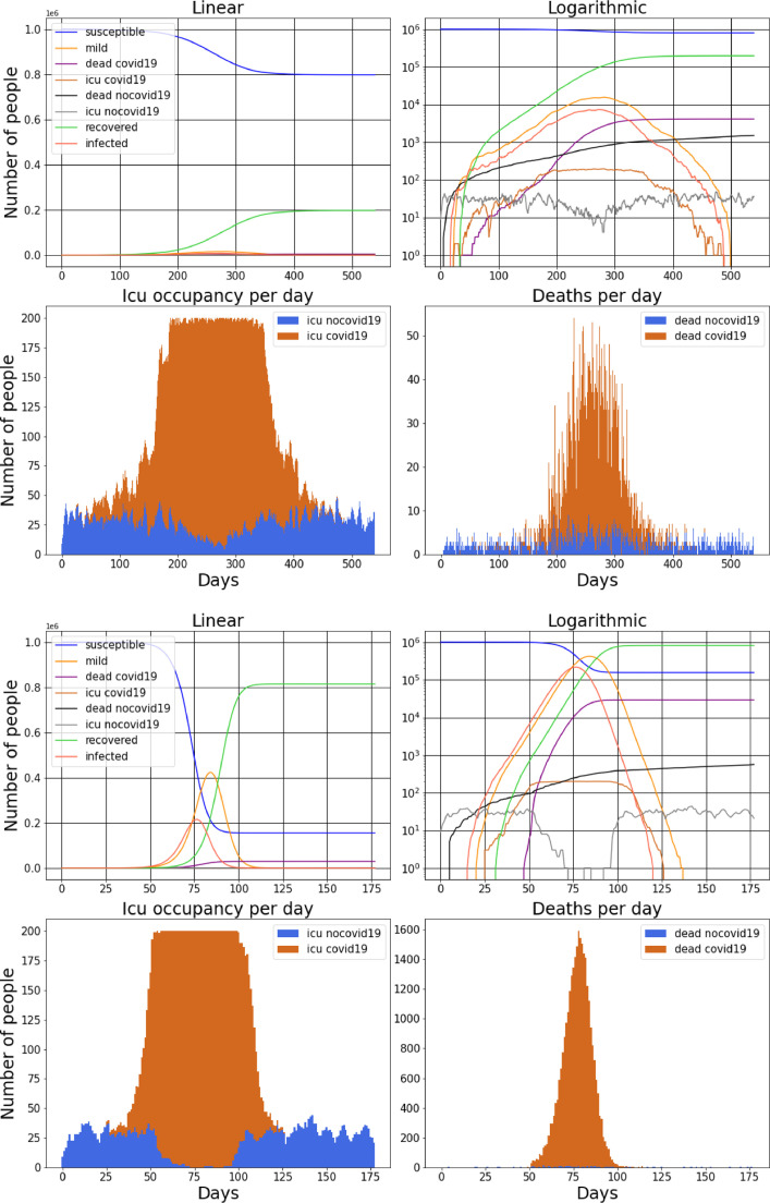
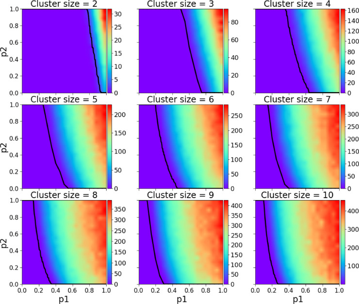
Before we compare the model’s simulation results with real data on the COVID-19 pandemic in Croatia, we show numerical simulations to become familiar with the general model’s properties. We start by analyzing the basic behavioural scenario, in Fig. 2 we present the parameter space of $p_1,p_2$ and the size of the clique/cluster $k$, the dependent variable is the daily average number of COVID-19 deaths during the pandemic. For two sets of model parameters in Fig. 3 (a) and (b) we present two arbitrarily chosen realisations where we show as in standard SIR models the numbers of susceptible individuals, infectious individuals, recovered individuals, and deceased individuals, where the cause of death is either COVID-19 or any other disease. As in the SIR model the individuals who have been infected and are capable of infecting susceptible individuals gradually increase reaching a maximum after which he number starts to diminish. In addition, we also show the number of mild individuals and patients in ICU (intensive care units) either due to COVID-19 or any other disease.

Fig. 2.

Daily average number of COVID-19 deaths during the course of the pandemic for $k$-clique/cluster sizes 2–10. The black line represents the maximum healthcare capacity (expressed in ICU units), left of the line the healthcare system was always functioning, right of it there was at least one simulation in which for at least one day the healthcare system was stressed with a too high demand. As expected the safest scenarios are the ones with smaller cluster sizes.

Fig. 3.

For two arbitrarily chosen realisations of model parameters we show the numbers of susceptible individuals, infected individuals, recovered individuals, deceased individuals, where the cause of death is either COVID-19 or another disease and individuals in ICU. In (a).3 - (b).3 we show the ICU occupancy and in (a).4 - (b).4 the deaths per day. It can be seen how during the peak of the pandemic the number of ICU patients non related to COVID-19 is highly reduced (due to the massive number of COVID-19 patients) but the deaths non related to COVID-19 are also increased (because untreated sick people die). Both (a).3 and (b).3 visually show two realisations where the healthcare system collapses (full capacity is reached). Both realisation are for cluster size = 4, the first having $p_1=0.4$, $p_2=0.65$ and the second $p_1=0.7$, $p_2=0.7$. It is clear how a higher probability of mobility $p_1$ results in much more severe daily deaths.

In (a).3-(b).3 and (a).4-(b).4 we separately point out the ICU patients and the dead for both COVID-19 and any other disease. Notice that at the peak of the pandemic the number of non-COVID-19 ICU patients decreases being relatively small in number to COVID-19 patients, this phenomenon has been noticed worldwide. As a consequence at the peak of the pandemic the number of non-COVID-19 deaths slightly increases because untreated people die.

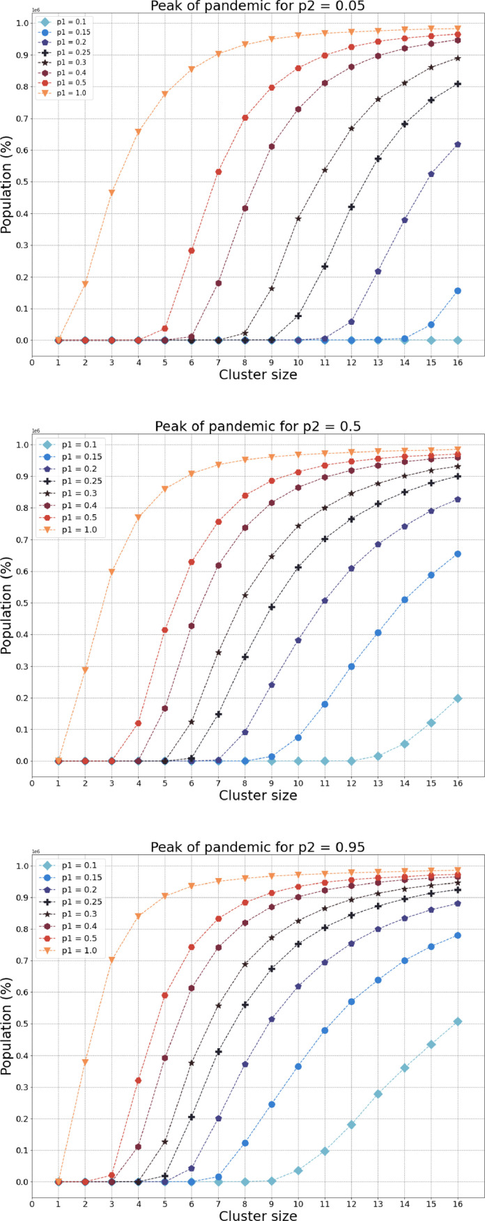
To this end in Fig. 4 for three arbitrarily choices of the probability of quarantine misbehaviour $p_2$, we demonstrate how the model’s peak of pandemic changes with the size of the cluster for varying choices of parameter $p_1$, which serves as a parameter of restrictions enforced by the government. Here, the lower (higher) value of $p_2$ characterises a nation where people more (less) strictly follow the government rules and suggestions regarding self-isolation. Similarly, the lower the value of $p_1$, the larger the government’s restrictions on communications outside the cluster, most commonly representing a family/household. Notice that for a country where its people strictly follow epidemiological and quarantine suggestions ($p_2=0.05$), for a high level of restrictions on mobility $(p_1=0.1)$ even for the largest size of the cluster the pandemic’s spread seems to be insignificant. Generally, comparing the (a) low and (b) high levels of $p_2$, for any choice of $p_1$ and the cluster size, the higher the level of quarantine misbehaviour, the pandemic looks more dreadful. Briefly, we vividly demonstrate that the model aims to substantially restrict the spread of the pandemic with both the number of local contacts inside the fundamental cluster and the population mobility – contacts outside the cluster i.e. in the central unit.

Fig. 4.

For two arbitrarily choices of the probability of quarantine misbehaviour $p_2$, we demonstrate how the models’ peak of pandemic changes with the size of the cluster for varying choice of parameter $p_1$. The model aims to substantially restrict the spread of pandemic with both the number of local contacts and contacts outside the cluster.

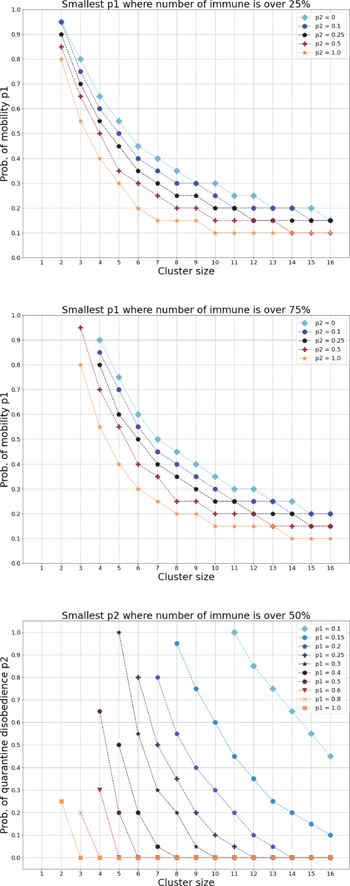
Our next simulations are related to natural herd immunity and here we test the model by identifying the smallest parameter $p_1$ for which at the end of the pandemic, the total number of immune (recovered) people is at least 25% or 75%. In Fig. 5 (a) the downmost curve represents a society where its population follows a strict non-compliance with self-isolation. Suppose we find the parameter value $p_1$ for a given cluster size for which the government measures yield at least 50% of immune individuals in the entire population. If the government decides to restrict the number of local contacts—thus, limiting the cluster size—what should be done with the number of contacts outside the cluster, controlled by the probability of mobility? As one should expect, reducing the number of local contacts may be accompanied by relaxing the restrictions on contacts outside the cluster in order to obtain the same percentage of immune individuals in the population. A decreasing functional dependence between the cluster size and the probability of mobility is exactly depicted in Fig. 5(a)-(b). Moving from the downmost curve to the uppermost curve, the latter representing a society whose population follows a strict compliance with self-isolation, for each cluster size the restrictions in contacts outside the cluster can be substantially relaxed in order to achieve the same epidemiological goal. In Fig. 5(c) we report a similar decaying functional dependence between the cluster size and the probability of quarantine misbehavior $p_2$ for a varying set of the probability of mobility. The higher variance of the level lines in (c) compared to (a)-(b) is an evidence that $p_1$ is the more expressive parameter compared to the quarantine misbehavior $p_2$.

Fig. 5.

(a)-(b) A decreasing functional dependence between the cluster size and the probability of mobility for a varying set of the probability of quarantine misbehaviour (disobedience). (c) A similar decaying functional dependence between the cluster size and the probability of quarantine misbehavior for a varying set of the probability of mobility.

3. Scenario comparison

A very efficient policy whose power is greatly underestimated is what we call the special group behavioural scenario. It simply means isolating in small communities (our $k$-cliques) the elderly or the risky parts of the population ($20\%-30\%$) while others still reduce their movements from what can be called normal behaviour when there is no pandemic. The key is to analyze the cost and benefits of this approach, where it is either just another unsuccessful way of dealing with disastrous pandemics or it is perhaps the key to reduce greatly the death toll while still allowing a certain degree of mobility by closing only the necessary.

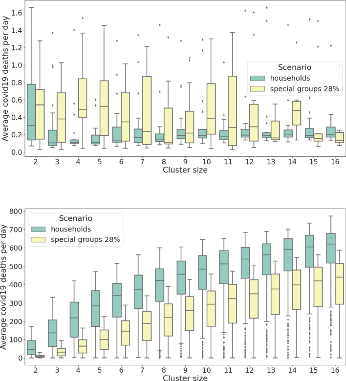
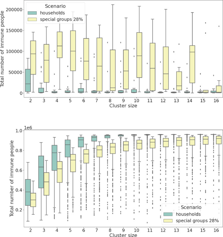
To this end, we compare the daily average number of COVID-19 deaths shown in Figs. 2 and 6 where it is clear that the latter presents a more efficient policy which can positively influence the relationship between the mobility of the population and the healthcare capacity (note that the area of collapse is smaller in Fig. 6 meaning that the black line is skewed to the right towards higher $p_1$ values). Figs. 7 and 8 vividly present the beneficial effects of the special group behavioural scenarios compared to the basic ones: Fig. 7(a) apparently shows that a higher number of people are expected to die on a daily basis in scenarios where the system remains functioning but, in fact, the conclusion is quite the opposite, indeed Fig. 8(a) shows that a much higher rate of people is exposed to COVID-19 at the end of the pandemic which means a much smaller overall death rate for the special group behavioural scenario (when adjusted with an average slightly longer pandemic of Fig. 9 ). Figs. 7(b) and 8(b) show that even when the system collapses, the death toll is still more than halved for a comparable level of people exposed to COVID-19 ($50\%$ less deaths against $10\%-15\%$ of less exposed people leads to a daily mortality decreased by $40\%$).

Fig. 6.

Daily average number of COVID-19 deaths during the course of the pandemic for $k$-clique/cluster sizes 2-10, for the risky groups behavioural scenario. Compared to Fig. 2 the daily death toll is greatly reduced and even the maximum healthcare capacity (especially for smaller cluster sizes) is reached for a higher combination of $p_1$ and $p_2$.

Fig. 7.

Average COVID-19 deaths per day (per million). Comparison between the basic behavioural scenarios and the special groups ones. (a) simulated data from the region of functioning healthcare system, the observed parameter for the two groups has different variance and slightly different median. (b) simulated data from the region of collapse, the observed parameter for the two groups has similar variance but significantly different median. Notice how there are more than two order of magnitudes of difference in daily deaths between (a) functioning healthcare and (b) collapsed healthcare. It is also interesting to notice in (b) the logarithmic relationship to the cluster size.

Fig. 8.

Total number of immune people (per million) at pandemic end. Comparison between the basic behavioural scenarios and the special groups ones. (a) simulated data from the region of functioning healthcare system, the observed parameter has significantly different variance and significantly different median. (b) simulated data from the region of collapse, the observed parameter has similar variance but different median.

Fig. 9.

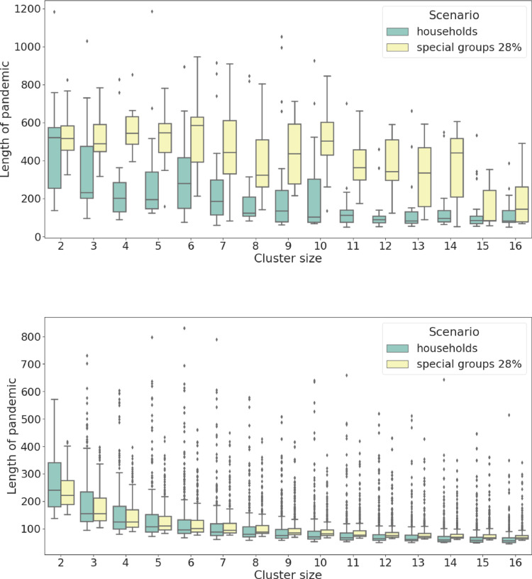
Length of pandemic (in days). Comparison between the basic behavioural scenarios and the special groups ones. (a) simulated data from the region of functioning healthcare system, the observed parameter has different variance and different median. (b) simulated data from the region of collapse, the observed parameter has similar variance and similar median. It is interesting to notice a decreasing functional dependence to the cluster size.

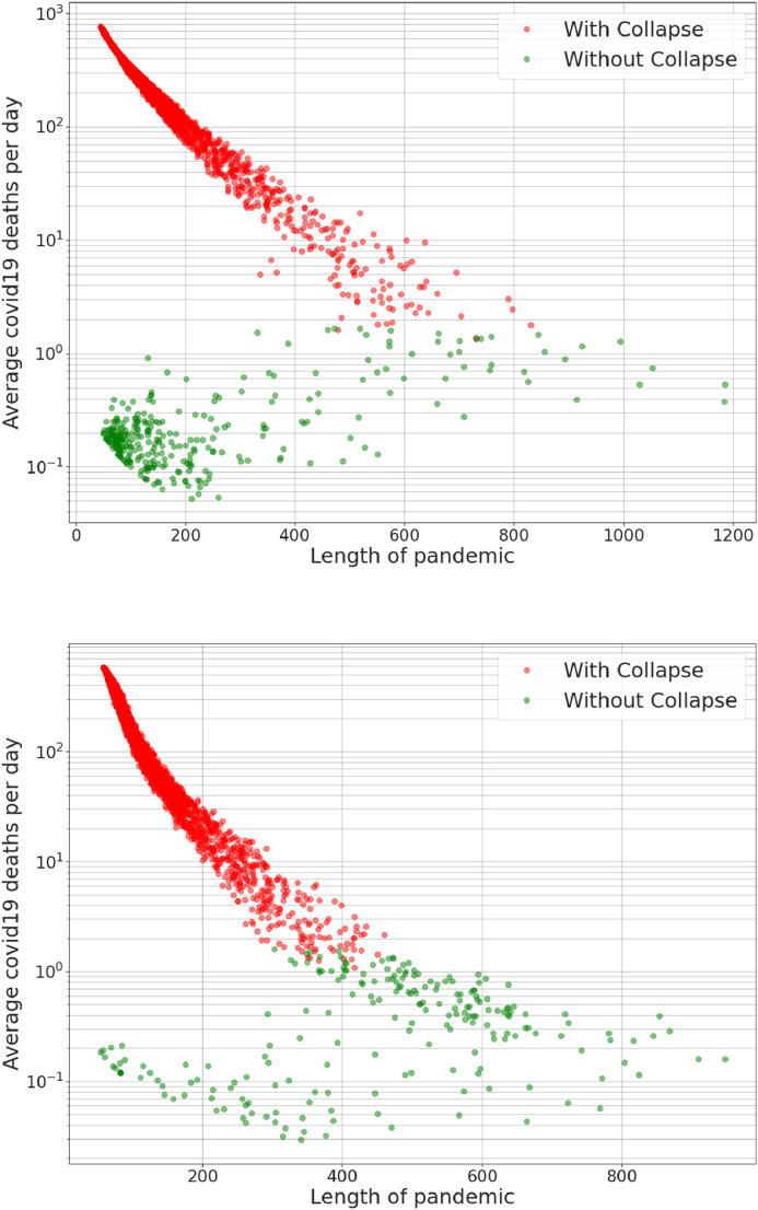
Fig. 9 presents the length (in days) of the pandemic simulations for the two behavioural scenarios: (b) shows that for collapsed scenarios the lengths are comparable and (a) reveals that for scenarios where the system remains functioning the pandemic tends to be longer. The latter claim is even more clear in Fig. 10 where we present a complex functional dependence between the length and the logarithm of the average COVID-19 deaths per day. Here, (a) refers to data for the basic behavioural scenarios while (b) refers to special group ones. It is very clear that in both behavioural cases the functional dependence is very different for the functioning and collapsed healthcare scenarios showing double clustering in (a) and a common decreasing functional dependence in (b). A very important observation is that in (b) all the collapsed healthcare scenarios tend to be much shorter than the functioning ones meaning that the special group behavioural policy is a type of flattening the curve policy (and therefore a pandemic prolongation policy).

Fig. 10.

Length of pandemic vs. logarithm of Average COVID-19 deaths per day (per million). Both graphs exhibit a very peculiar and complex dependence of the two variables; (a) presents data from basic behavioural scenarios; two main clusters can be observed one from the scenarios with functioning healthcare system (without collapse) and the other from the scenarios in collapse. Both the clusters happen for very short pandemics but with very different death rates. (b) presents data from special groups behavioural scenarios; only one cluster can be observed related to the scenarios in collapse while the data related to the functioning healthcare system (without collapse) is somehow shifted towards the same functional dependence of the scenarios in collapse. Another important difference is that in (b) there are not scenarios in collapse where the pandemic is longer than 450 days while in (a) there are several even above 600 days in length. Meaning that for the special groups behavioural scenarios all the simulations where the pandemic lasts the longest (the infection curve is successfully flattened) have never reached healthcare collapse.

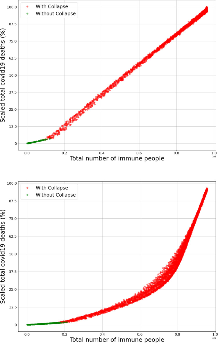
Fig. 11 presents the functional dependence between the mortality (expressed as a percentage of the maximum expected mortality) and the number of immune people at the end of the pandemic. (a) is related to data from the basic behavioural scenarios and (b) to special groups, let’s call these functions $f$ an $g$ respectively. Firstly, we notice that $f\left(x\right)<g\left(x\right)$ for every $x$ confirming that special groups behavioural scenarios lead to an inferior overall mortality rate. Secondly, the discontinuity of the first kind in the first derivative of $f$ is emblematic and shows a drastic (more than double) change of slope when the healthcare system collapses. In $g$ the discontinuity is still present but much less extreme, meaning that the special groups behavioural scenarios have an important smoothing effect even for collapsed zones; however, after $x=70\%$ the slope becomes very steep and $g$ catches up $f$ at around $x=95\%$ meaning that isolating the risky groups and the elderly without reducing the mobility at all is counterproductive.

Fig. 11.

Total number of immune people vs. total COVID-19 deaths (scaled in percentage with the maximum number of deaths obtained in the simulations). Both graphs present an increasing functional dependence between the two variables; (a) presents data from basic behavioural scenarios; the data from scenarios with functioning healthcare system (without collapse) and scenarios in collapse lie on two different linear functions with a discontinuity of the first kind in the first derivative which is an emblematic representation of the healthcare system collapse (individuals which could be saved start to die). (b) presents data from special groups behavioural scenarios; the data from scenarios with functioning healthcare system (without collapse) lie on an even less deadly linear function compared to the one in (a) (the slope of the line is smaller). Notice that $f\left(x\right)<g\left(x\right)$ for every $x$, where $f$ represents the function in (a) and $g$ in (b) reconfirming that the special groups behavioural scenario is expected to be significantly less deadly in every possible scenario. It is interesting to notice that $g$ is not linear and a smoothing effect is present, also around $x=70\%$ the slope of the mortality increases rapidly (due to the fact that a large portion of risky clusters becomes infected).

4. Prediction of epidemic bursts

Finally, we exemplify our model with real data on the Croatian COVID-19 pandemic. Until now all the simulations and analyses where made for a set of fixed values of parameters $p_1,p_2$, and the cluster size $k$. However, reality is much more complex and while it is quite reasonable to assume that the number of people per household is constant during a pandemic, since the demographic rate is quite moderate in many countries, it is definitely not correct to consider the probability of mobility $p_1$ and the probability of quarantine misbehaviour $p_2$ as constant.

The level of generalization of our parameter of mobility $p_1$ is very wide and the best approximation of it is a general movement of the population. Among many options one can choose from, for the proxy for $p_1$ we choose the Stringency index developed by the University of Oxford [46], where we define the link between the parameter $p_1$ and the stringency $s$ in a straightforward way:

$$p_1=1-\frac{s}{100}$$ (2)

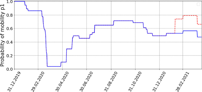
Fig. 12 shows the temporal changes of $p_1$ for Croatia as defined in (2). The vast majority of the model parameters, including the cluster size $k=3$ which corresponds to the size of the average Croatian household [47], are fixed from empirical data.

Fig. 12.

Probability of mobility for Croatia as described in Eq. (2), blue line. The assumed sudden change where Eq. (4) and $\alpha =1.4$ applies starts around the middle of February, red line. (For interpretation of the references to colour in this figure legend, the reader is referred to the web version of this article.)

The inherently unknown parameters are $p_2$ which quantifies the level of a country’s disobedience and the IFR (infection fatality rate) of COVID-19 for which it is assumed to be within the range $0.1\%-2\%$. Using a simplified basic behavioural model where only COVID-19 states (without U and N) and fixing $p_1$ and $k$ as above we use a Bayesian optimization (BO) to identify $p_2$ and IFR which will yield the best fit for the Croatian mortality data.

Bayesian optimization is a sequential search algorithm designed to find the global minimizer or maximizer of an unknown non-analytic or oracle function $f$ whose gradient is also analytically unknown

$${\mathbf{x}}^{*}=\arg \underset{\mathbf{x}}{\min }f\left(\mathbf{x}\right)$$ (3)

BO requires two components: a model that approximates $f$ and an acquisition function, $\alpha \left(\mathbf{x}\right)$ that quantifies the informational gain [48], [49]. Here, we use Gaussian process (GP) models as the probabilistic models in order to approximate the average number of deaths.

The function $f$ we minimize is the root mean squared error RMSE between the empirical (14 day moving averaged) COVID-19 deaths and the simulated ones over the set $A$, that is a rectangle formed by the ranges of IFR and $p_2$ ($A=[0.1,2]\times [0,1]$).

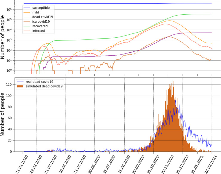
We use the upper confidence bound (UCB) as the acquisition function with 30 initial random points and 70 descent points. The algorithm successfully converges and the values that best fit the data for the thirteen months period are $p_2=24.6\%$ and IFR=$1.4\%$, see Table 1 for more details regarding the parameters. Fig. 13(b) shows the results of the optimization procedure compared to the empirical data on COVID-19 daily deaths for these months, since the outbreak in Croatia. We find a fascinating agreement between the model and empirical results, where the timing when the pandemic bursts is very accurately predicted. In Fig. 13 (a) we show the curves representing the numbers of susceptible, infected, mild, COVID-19 dead, ICU COVID-19 patients and recovered individuals simulated by the model.

Table 1.

Parameter values. The table shows the value of each parameter of the model which was fixed to comply with empirical findings. The free (unknown) parameters found by the BO algorithm are $p_2=24.6\%$ and IFR$=1.4\%$ ($\zeta =2.8\%$ and $\gamma =1-\zeta$).

Croatian model parameters
Parameter	Value	Description	Source
$p_1$	Eqs. (2) and (4)	Probability of mobility	[46]
$k$	3	Cluster size	[47]
$\kappa$	2.5	Rate of intensity of contacts in the central unit	[40]
$r$	$10\%$	Probability of disease transmission	[35]
$\theta$	$50\%$	Mortality rate for ICU patients	[37]
$\eta$	$1-\theta$	Survival rate for ICU patients	[37]
$\delta$	$\approx 100\%$	Survival rate for mild cases	[36], [37]
${\tau }_1,{\tau }_3$	5 days	Time for onset of symptoms	[38]
${\tau }_4,{\tau }_5$	10 days	Time of stay in ICU	[38], [39]
${\tau }_2$	11 days	Time for recovery	[39]

Fig. 13.

Empirical and simulated deaths. (a) Curves represent the numbers of susceptible, mild, COVID-19 dead, ICU COVID-19 patients, recovered and infected. (b) Comparison of daily COVID-19 deaths between the model and the empirical results, the timing of the pandemic bursts is in well agreement with the model simulation.

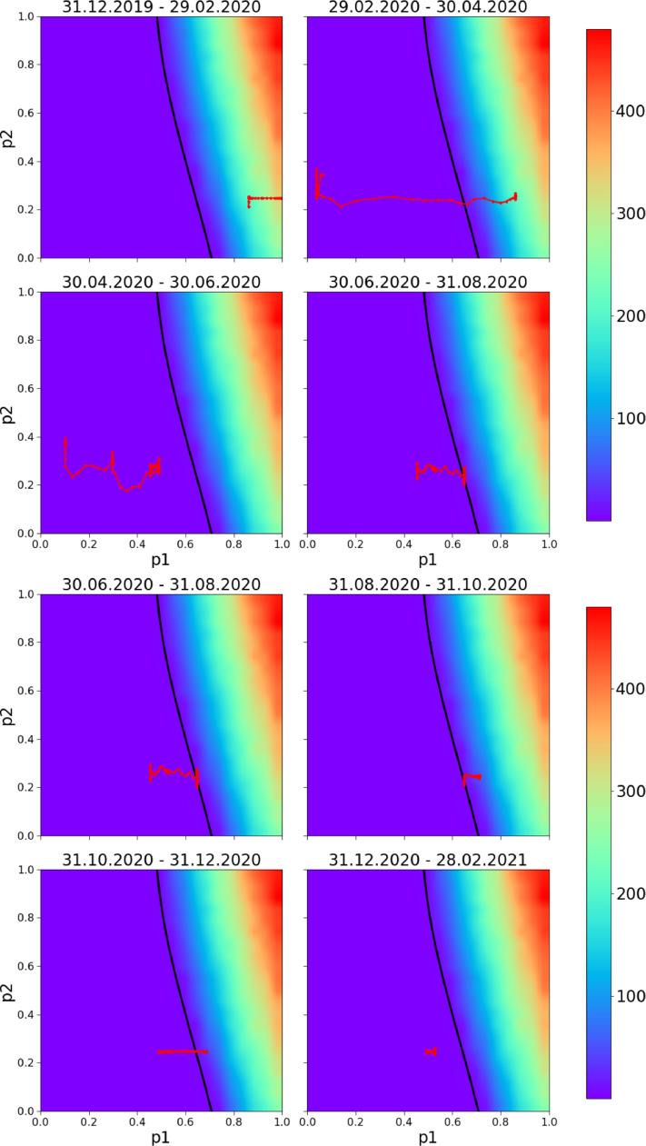
The sample local-time realisations of parameters $p_1\left(t\right)$ and $p_2\left(t\right)$ are different and fluctuate around the population parameters $p_1$ and $p_2$. Therefore we perform numerical simulations [32] for our network and analyse how a policy random walker represented by a pair $(p_1\left(t\right),p_2\left(t\right))$ fluctuates in the phase space. Fig. 14 shows a phase diagram with 2-month period of policy changes in Croatia: $p_1$ is fixed according to Eq. (2) and $p_2$ is obtained from the Bayesian optimization showed in the context of expected daily deaths (similar to Fig. 2 but adjusted for Croatia). The black line represents the healthcare capacity of Croatia in terms of ICU units. It is very interesting to notice that starting from the beginning of the pandemic from mid-February 2021, whenever the policy walker is on the left of the line, the pandemic is controlled. In contrast, when the policy random walker crosses the line the pandemic starts to grow exponentially. Namely, observing both Figs. 13 and 14 it is clear that the policy walker was in the catastrophe zone between the end of August and mid-November which is exactly when the pandemic started to grow again with a peak in deaths reached with a delay of around $\tau =3$ weeks. This approach has an obvious predicting power because the policy random walker was within the range $10-80$ with a peak of 100 expected deaths per day which is exactly what happened. Note that 100 deaths in Croatia corresponds to 8000 in the USA.

Fig. 14.

Predicting bursts. The walking line is the local-time 7 day moving averaged realisation of parameters $p_1\left(t\right)$ and $p_2\left(t\right)$ applying eq.(2) for fourteen month period (blue line in Fig. 12). It represents very plausible changes of the parameters $p_1$ and $p_2$ for Croatia for 2-month periods. The background variable is the expected number of COVID-19 deaths per day, the model fits very well the empirical data: the pandemic starts to grow exponentially as soon as the walker crosses the black line and enters the catastrophe zone; pandemic bursts are successfully predicted and parametrically visualized. (For interpretation of the references to colour in this figure legend, the reader is referred to the web version of this article.)

While short-term predictions can be almost read from the graph, putting $f\left(x\right)$ as the number of predicted daily deaths for a given pair of parameters $x=(p_1,p_2)$ and integrating $g\circ f$ over the walking line (for $g$ empirically found and exponential in nature) very accurate long-term predictions are also possible.

4.1. Multiple waves prediction

Recently Croatia was hit by the third wave of COVID-19 infection which significantly worsened the epidemiological situation. Arguably, as time passes by, more and more individuals start to resist to the policy measures (recovered individuals, individuals economically hit or individuals which simply wish to return to normality all tend to influence their surroundings to not follow the policies and regulations). As shown, we modelled these changes in behaviour through the parameters $p_1$ and $p_2$, more precisely an increased misbehaviour is directly represented by an increased parameter $p_2$, but if the change becomes structural, the relationship in (2) can change. In other words the stringency $s$, which is a representation of the strictness of the policy adopted by the government, and the effective mobility adopted by the individuals $p_1$ tend to be more disconnected, where a more suitable equation is therefore

$$p_1=\alpha (1-\frac{s}{100}).$$ (4)

If $0<\alpha <1$ it means that the individuals behave even more strictly than what is suggested by the government, therefore further reducing their mobility. In contrast, if $\alpha >1$ the individuals tend not to follow the government policy and move and behave more freely. The case $\alpha =1$ leads back to (2). In the model we assume that the individuals suddenly and structurally start to move more freely which is in our model reflected in sudden changes of parameters $p_1$ and $p_2$.

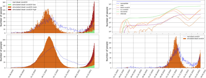
Around the middle of February the Croatian daily COVID-19 cases dropped drastically and this change in the pandemic was followed by large demonstrations supporting a return to normality. Nevertheless, a couple of weeks later new cases and new deaths started to rise again and a third wave was declared by the authorities. Fig. 15 (a) and (b) shows the progress of the Croatian COVID-19 daily deaths with an emphasis on the beginning of the third wave in March-April. The three curves are obtained by altering the parameter $p_2$ found by the BO algorithm (for the January 2020 - February 2021 period). Shown is the curve in green with a $40\%$ increased parameter that is the most favourable one; shown are the curves with $p_2$ increased by $120\%$ (orange) and $180\%$ (red). All three curves are generated with $\alpha =1.4$ starting from the middle of February (see red line in Fig. 12) which suggests the possibility of a structural change in the response to the policies by the individuals. Adding the parameter $\alpha$ as well as slicing the historical data into regions that allow different $p_2$’s and minimizing with BO each region separately is a straightforward extension with a proven capability of predicting and simulating multiple pandemic waves. Fig. 15(c) and (d) shows the complete pandemic with all three pandemic waves together with the model output since the COVID-19 outbreak in Croatia, sudden increases in the probability of quarantine misbehaviour and the probability of mobility for the third wave generate good agreement with daily COVID-19 deaths.

Fig. 15.

Empirical and simulated deaths. (a)-(b) Comparison of daily COVID-19 deaths between the model and the empirical results between August and April. After February three different curves are shown: in the green and least aggressive scenario the parameter $p_2$ found by the BO algorithm was increased by $40\%$ in the medium scenario by $120\%$ and in the red and most aggressive by $180\%$. All three scenarios are generated with $\alpha =1.4$ starting from the middle of February suggesting that the individuals probably started to follow the policies less strictly. (a) shows daily deaths data. (b) 14 day moving averaged deaths data. (c)-(d) Comparison since the outbreak in Croatia. (c) Curves represent the simulated numbers of susceptible, mild, COVID-19 dead, ICU COVID-19 patients, recovered and infected. (d) Comparison of daily COVID-19 deaths between the model and the empirical results, after February the middle curve of (a) is added. The timing of all three pandemic waves are in good agreement with the model simulation.

5. Conclusion

Motivated by the importance of public trust in the government and its institutions during a pandemic, we propose a new dynamical network model based on mobility restrictions and quarantine disobedience, the model has shown the ability to successfully expose empirical evidence of COVID-19 pandemic waves. We showed that pandemic waves are driven by both changes in mobility restrictions and quarantine disobedience.

The application of the model was demonstrated on Croatian COVID-19 empirical data by setting the probability of mobility parameter according to the Oxford’s Stringency Index while calibrating the probability of quarantine disobedience parameter with Bayesian optimization in order to obtain the best alignment of model output with real COVID-19 deaths data. We showed in different two months pandemic periods how the optimized parameter for probability of quarantine disobedience changes along with Stringency Index data enforced probability of mobility. The calibrated model gives good alignment in all three empirically observed pandemic waves in Croatia with interesting insights. We can interpret that the first two pandemic waves were subject to quarantine disobedience while the last was due to a more structural change in people’s mobility (quarantine disobedience alone seems not enough to explain such surge in cases).

Applying the model for Croatian COVID-19 pandemic scenario (which has a rather complex appearance of pandemic waves) it was even enough to calibrate the probability of quarantine disobedience with respect to only new daily deaths data. However, expressiveness of our model also allows that instead of applying Bayesian optimization with the objective to best fit the prediction for only dead daily cases, the use of a more complex multidimensional objective function which alongside the daily deaths also looks for the best fit of the daily hospitalized, ICU patients, the growth rate of new cases etc. This approach could be beneficial for more complex other countries’ pandemic scenarios or used for exploring the level of a more generalized global pandemics dynamics.

Moreover, the interplay between the mobility $p_1$ and the quarantine misbehaviour which models the disobedience of the population $p_2$ could be in addition incorporated in the model by enforcing their functional dependence which can be approximated through a deeper analysis of country-scale or world-scale empirical data. For example, $p_2$ is naturally linked to the general trust in the government by the people which is changeable but perhaps related to other indexes like the level of corruption or the quality of life. For some future pandemics our study may help policy makers understand how to suitably identify high disobedience individuals, quantify their risk, in order to lower, as much as possible, the economic and social losses of pandemics.

Declaration of Competing Interest

The authors declare that they have no known competing financial interests or personal relationships that could have appeared to influence the work reported in this paper.

References

- 1.Cirillo P., Taleb N.N. Tail risk of contagious diseases. Nat Phys. 2020;16:606–613. [Google Scholar]
- 2.Andersen K.G., Rambaut A., Lipkin W.I., Holmes E.C., Garry R.F. The proximal origin of SARS-CoV-2. Nat Med. 2020;26:450–452. doi: 10.1038/s41591-020-0820-9. [DOI] [PMC free article] [PubMed] [Google Scholar]
- 3.Miller I.F., Becker A.D., Grenfell B.T., Metcalf C.J.E. Disease and healthcare burden of COVID-19 in the United States. Nat Med. 2020;26:1212–1217. doi: 10.1038/s41591-020-0952-y. [DOI] [PubMed] [Google Scholar]
- 4.Callaway E. Coronavirus vaccine trials have delivered their first results, but their promise is still unclear. Nature. 2020;581:363–364. doi: 10.1038/d41586-020-01092-3. [DOI] [PubMed] [Google Scholar]
- 5.McKee M., Stuckler D. If the world fails to protect the economy. COVID-19 will damage health not just now but also in the future. Nat Med. 2020;26:640–642. doi: 10.1038/s41591-020-0863-y. [DOI] [PubMed] [Google Scholar]
- 6.Bjornstad O.N., Shea K., Krzywinski M., Altman N. Modeling infectious epidemics. Nat Methods. 2020;17:455–456. doi: 10.1038/s41592-020-0822-z. [DOI] [PubMed] [Google Scholar]
- 7.Bjornstad O.N., Shea K., Krzywinski M., Altman N. The SEIRS model for infectious disease dynamics. Nat Methods. 2020;17:557–558. doi: 10.1038/s41592-020-0856-2. [DOI] [PubMed] [Google Scholar]
- 8.Flaxman S., et al. Estimating the effects of non-pharmaceutical interventions on COVID-19 in Europe. Nature. 2020;584:257–261. doi: 10.1038/s41586-020-2405-7. [DOI] [PubMed] [Google Scholar]
- 9.Legido-Quigley H., et al. Are high-performing health systems resilient against the COVID-19 epidemic? Lancet. 2020;395(10227):848–850. doi: 10.1016/S0140-6736(20)30551-1. [DOI] [PMC free article] [PubMed] [Google Scholar]; Epub 2020 March 6.
- 10.IHME COVID-19 forecasting team. 2020. Modeling COVID-19 scenarios for the United States Nature Medicine. [DOI] [PMC free article] [PubMed]
- 11.Maier B., Dirk F.B. Effective containment explains subexponential growth in recent confirmed COVID-19 cases in china. Science. 2020;368(6492):742–746. doi: 10.1126/science.abb4557. [DOI] [PMC free article] [PubMed] [Google Scholar]
- 12.Tegnell A. Closing borders is ridiculous: the epidemiologist behind Sweden’s controversial coronavirus strategy. Nature. 2020;580:574. doi: 10.1038/d41586-020-01098-x. [DOI] [PubMed] [Google Scholar]
- 13.Kermack W.O., McKendrick A.G. A contribution to the mathematical theory of epidemics. Proc R Soc Lond A. 1927;115:700–721. [Google Scholar]
- 14.Pastor-Satorras R., Vespignani A. Epidemic spreading in scale-free networks. Phys Rev Lett. 2001;86:3200. doi: 10.1103/PhysRevLett.86.3200. [DOI] [PubMed] [Google Scholar]
- 15.Adamic K., Huberman B.A. Internet: Growth dynamics of the world-wide web. Nature. 1999;401:131. [Google Scholar]
- 16.Garlaschelli D., Caldarelli G., Pietronero L. Universal scaling relations in food webs. Nature. 2003;423:165. doi: 10.1038/nature01604. [DOI] [PubMed] [Google Scholar]
- 17.Pastor-Satorras R., Castellano C., Van Mieghem P., Vespignani A. Epidemic processes in complex networks. Rev Mod Phys. 2015;87(14):925–979. [Google Scholar]
- 18.De Domenico M., Granell C., Porter M.A., Arenas A. Te physics of spreading processes in multilayer networks. Nat Phys. 2016;12:901–906. [Google Scholar]
- 19.Fararo T. Biased networks and the strength of weak ties. Soc Netw. 1983;5:1–11. [Google Scholar]
- 20.Zaric G.S., Random V.S. nonrandom mixing in network epidemic models. Health Care Manag Sci. 2002;5:147–155. doi: 10.1023/a:1014489218178. [DOI] [PubMed] [Google Scholar]
- 21.Eubank S., Guclu H., Anil Kumar V.S., Marathe M.V., Srinivasan A., Toroczkai Z., Wang N. Modeling disease outbreaks in realistic urban social networks. Nature. 2004;429:180–184. doi: 10.1038/nature02541. [DOI] [PubMed] [Google Scholar]
- 22.Del Valle S.Y., Hyman J.M., Eubank S.G., Hethcote H.W. Mixing patterns between age groups using social networks. Soc Netw. 2007;29:539–554. [Google Scholar]
- 23.Rapoport A., Yuan Y., Kochen M. The Small World. Ablex; Norwood, NJ: 1989. Some aspects of epidemics and social nets; pp. 327–348. [Google Scholar]
- 24.Chang S., Pierson E., Koh P.W., et al. Mobility network models of COVID-19 explain inequities and inform reopening. Nature. 2021;589:82–87. doi: 10.1038/s41586-020-2923-3. [DOI] [PubMed] [Google Scholar]
- 25.Kretzschmar M., Morris M. Measures of concurrency in networks and the spread of infectious diseases. Math Biosci. 1996;133:165–195. doi: 10.1016/0025-5564(95)00093-3. [DOI] [PubMed] [Google Scholar]
- 26.Chinazzi M., et al. The effect of travel restrictions on the spread of the 2019 novel coronavirus (COVID-19) outbreak. Science. 2020;368:395–400. doi: 10.1126/science.aba9757. [DOI] [PMC free article] [PubMed] [Google Scholar]
- 27.Zlatic V., Barjasic I., Kadovic A., Stefancic H., Gabrielli A.. Bi-stability of SUDR+k model of epidemics and test kits applied to COVID-19. [DOI] [PMC free article] [PubMed]
- 28.Chang S., Pierson E., Koh P.W., Gerardin J., Redbird B., Grusky D., Leskovec J. Mobility network models of COVID-19 explain inequities and inform reopening. Nature. 2020 doi: 10.1038/s41586-020-2923-3. [DOI] [PubMed] [Google Scholar]
- 29.Chande A., Lee S., Harris M., Nguyen Q., Beckett S.J., Hilley T., Andris C. Real-time, interactive website for US-county-level COVID-19 event risk assessment. Nat Hum Behav. 2020;4:1313–1319. doi: 10.1038/s41562-020-01000-9. [DOI] [PMC free article] [PubMed] [Google Scholar]
- 30.Alban A., Chick S.E., Dongelmans D.A., Vlaar A.P.J. ICU capacity management during the COVID-19 pandemic using a process simulation. Intensive Care Med. 2020;46:1624–1626. doi: 10.1007/s00134-020-06066-7. [DOI] [PMC free article] [PubMed] [Google Scholar]
- 31.Cinelli M., Quattrociocchi W., Galeazzi A., Valensise C.M., Brugnoli E., Schmidt A.L., Zola P., Zollo F., Scala A. The COVID-19 social media infodemic. Sci Rep. 2020;10 doi: 10.1038/s41598-020-73510-5. [DOI] [PMC free article] [PubMed] [Google Scholar]; Article number: 16598
- 32.Majdandzic A., Podobnik B., Buldyrev S.V., Kenett D., Havlin S., Stanley H.E. Dynamical networks with spontaneous recovery. Nat Phys. 2014;10(1):34–38. [Google Scholar]
- 33.Jusup M., et al. “Dynamically rich, yet parameter-sparse models for spatial epidemiology: comment on coupled disease-behavior dynamics on complex networks: a review by Z.” wang et al. Phys Life Rev. 2015;15:43–46. doi: 10.1016/j.plrev.2015.09.006. [DOI] [PubMed] [Google Scholar]
- 34.COVID-19 Dashboard by the Center for Systems Science and Engineering (CSSE) at Johns Hopkins University (JHU).
- 35.Chu D.K., Akl E.A., Duda S., Solo K., Yaacoub S., Schünemann H.J., et al. Physical distancing, face masks, and eye protection to prevent person-to-person transmission of SARS-CoV-2 and COVID-19: a systematic review and meta-analysis. Lancet. 2020;395:1973–1987. doi: 10.1016/S0140-6736(20)31142-9. [DOI] [PMC free article] [PubMed] [Google Scholar]
- 36.European centre for disease prevention and control (ECDC). 2020. Coronavirus disease 2019 (COVID-19) in the EU/EEA and the UK - ninth update. https://www.ecdc.europa.eu/en/publications-data/rapid-risk-assessment-coronavirus-disease-2019-covid-19-pandemic-ninth-update(23 Apr 2020)
- 37.Abate S.M., Ahmed Ali S., Mantfardo B., Basu B. Rate of intensive care unit admission and outcomes among patients with coronavirus: a systematic review and meta-analysis. PLoS One. 2020;15(7):E0235653. doi: 10.1371/journal.pone.0235653. [DOI] [PMC free article] [PubMed] [Google Scholar]
- 38.World health organization (WHO). 2020. Report of the WHO-China joint mission on coronavirus disease 2019 (COVID-19). https://www.who.int/docs/default-source/coronaviruse/who-china-joint-mission-on-covid-19-final-report.pdf.
- 39.Zhou F., Yu T., Du R., Fan G., Liu Y., Liu Z., et al. Clinical course and risk factors for mortality of adult inpatients with COVID-19 in Wuhan, China: a retrospective cohort study. Lancet. 2020;295:1054. doi: 10.1016/S0140-6736(20)30566-3. [DOI] [PMC free article] [PubMed] [Google Scholar]
- 40.Liu Y., Gayle A.A., Wilder-Smith A., Rocklöv J. The reproductive number of COVID-19 is higher compared to SARS coronavirus. J Travel Med. 2020;13(2):27. doi: 10.1093/jtm/taaa021. [DOI] [PMC free article] [PubMed] [Google Scholar]; Taaa021. doi: 10.1093/jtm/taaa021. PMID: 32052846; PMCID: PMC7074654
- 41.Andres E., et al. Evolution of mortality over time in patients receiving mechanical ventilation. ATS J. 2013 doi: 10.1164/rccm.201212-2169OC. [DOI] [PubMed] [Google Scholar]
- 42.Data on hospital and ICU admission rates and current occupancy for COVID-19. URL: https://www.ecdc.europa.eu/en/publications-data/download-data-hospital-and-icu-admission-rates-and-current-occupancy-covid-19.
- 43.Pavan K.B., et al. Covid-19 in critically ill patients in the seattle region — case series. New Engl J Med. 2020 doi: 10.1056/NEJMoa2004500. [DOI] [PMC free article] [PubMed] [Google Scholar]
- 44.Onder G., i G.R., Brusaferro S. Case-fatality rate and characteristics of patients dying in relation to COVID-19 in italy. Jama. 2020 doi: 10.1001/jama.2020.4683. [DOI] [PubMed] [Google Scholar]
- 45.Coronavirus cases. URL: https://www.worldometers.info/coronavirus/.
- 46.Stringency index. URL: https://ourworldindata.org/grapher/covid-stringency-index.
- 47.Eurostat. Average number of persons per household by household composition, number of children and age of youngest child. URL: https://ec.europa.eu/eurostat/databrowser/view/lfst_hhantych/default/table?lang=en.
- 48.Vargas-Hernandez R.A. Bayesian optimization for calibrating and selecting hybrid-density functional models. J Phys Chem A. 2020;124(20):4053–4061. doi: 10.1021/acs.jpca.0c01375. [DOI] [PubMed] [Google Scholar]
- 49.Sha D., Ozbay K., Ding Y. Applying Bayesian optimization for calibration of transportation simulation models. Transp Res Rec. 2020;2674(10):215–228. doi: 10.1177/0361198120936252. [DOI] [Google Scholar]