Robustness of epithelial sealing is an emerging property of local ERK feedback driven by cell elimination

Summary

What regulates the spatiotemporal distribution of cell elimination in tissues remains largely unknown. This is particularly relevant for epithelia with high rates of cell elimination where simultaneous death of neighboring cells could impair epithelial sealing. Here, using the Drosophila pupal notum (a single-layer epithelium) and a new optogenetic tool to trigger caspase activation and cell extrusion, we first showed that death of clusters of at least three cells impaired epithelial sealing; yet, such clusters were almost never observed in vivo. Accordingly, statistical analysis and simulations of cell death distribution highlighted a transient and local protective phase occurring near every cell death. This protection is driven by a transient activation of ERK in cells neighboring extruding cells, which inhibits caspase activation and prevents elimination of cells in clusters. This suggests that the robustness of epithelia with high rates of cell elimination is an emerging property of local ERK feedback.

Graphical abstract

Highlights

• •Simultaneous elimination of three neighboring cells is detrimental for epithelia
• •Biased cell-death distribution prevents the appearance of such clusters
• •This bias is driven by ERK pulses and caspase inhibition in the neighbors of dying cells
• •Clusters of elimination and transient sealing defects appear upon EGFR/ERK inhibition

How epithelia fine-tune the spatiotemporal distribution of cell death and cope with high rates of elimination remains unclear. Valon et al. shows that pulses of ERK induced near every dying cell prevent the simultaneous elimination of neighboring cells, hence maintaining epithelial sealing despite the high rates of cell elimination.

Introduction

Epithelial robustness is essential for the mechanical and chemical integrity of metazoan organs. This stability relies on strong mechanical coupling between cells and cell sealing through adherens junctions and septate junctions (Guillot and Lecuit, 2013). Yet, this robustness is constantly challenged by the dynamic nature of epithelia, which undergo rapid turnover during homeostasis (Patterson and Watson, 2017), have high elimination rates during morphogenesis (Eisenhoffer et al., 2012; Marinari et al., 2012; Monier et al., 2015; Ninov et al., 2007; Toyama et al., 2008), or high rates of cell elimination induced by variations in the environment (Loudhaief et al., 2017; O'Brien et al., 2011). Despite cell removal, cohesion of the tissue can be maintained through cell extrusion, which coordinates the detachment of one cell from the layer either apically or basally with the emergence of new junctions between the remaining cells (Gudipaty and Rosenblatt, 2017; Ohsawa et al., 2018). However, this process has been studied mostly under conditions where cells are removed individually. Whether concomitant elimination of neighboring cells could impair extrusion and tissue cohesion remains unclear. Yet, such configuration is very likely to occur in conditions of high cell elimination rates: for instance, more than 1,000 enterocytes are eliminated every 24 h from a single villus of the mouse small intestine (Williams et al., 2015), while the entire epithelial layer can be removed in less than 24 h during development, as in the Drosophila pupal abdomen (Ninov et al., 2007). However, in many instances the exact spatiotemporal distribution of cell death is not known and the putative mechanisms orchestrating this distribution have not been studied.

Here, to address these questions, we used the Drosophila pupal notum, a single-layer epithelium that undergoes high rate of extrusions in some regions (Levayer et al., 2016; Marinari et al., 2012). First, using a new optogenetic tool to trigger caspase activation and extrusion, we showed that elimination of clusters of three or more cells is sufficient to impair extrusion and epithelial sealing. By combining statistical analysis and modeling, we then showed that such clusters are avoided through a local protective phase following each cell elimination. This protection is driven by pulses of ERK activity in cells neighboring dying cells, which prevent/revert caspase activation. Altogether, this study demonstrates that the spatiotemporal distribution of cell death is an emerging property of local ERK pulses, which are essential for epithelial robustness.

Results

Simultaneous elimination of at least three cells in cluster is detrimental for the tissue

First, we asked whether concomitant extrusion of several neighboring cells impairs the maintenance of epithelial sealing. As such, we developed a UAS-optoDronc Drosophila line, which can trigger rapid caspase activation through blue-light-induced clustering of caspase-9 (Figures 1A and S1A). Expression of optoDronc in fly eyes (GMR-gal4 eye-specific driver) is sufficient to trigger cell death upon blue-light exposure and can be rescued by expression of the downstream effector caspase inhibitor, p35 (Figure S1B). Subsequently, we used the Drosophila pupal notum to assess the efficiency of the construct in triggering epithelial cell elimination. Blue-light exposure of clones expressing optoDronc triggers elimination of the majority of cells in less than 1 h (Figures 1B, S1C, and S1E; Video S1A). OptoDronc-triggered extrusions are similar to physiological extrusions in the pupal notum, albeit slightly faster (Figure S1F) and require effector caspase activation (Figures S1D and S1E; Video S1A) like physiological extrusions in the notum (Levayer et al., 2016; Moreno et al., 2019). We then induced concomitant elimination of groups of cells of various sizes and shapes by expressing optoDronc in clones. While extrusions of single cells or several cells in lines occurred normally (Figures 1B, 1E, and 1F; Video S1C left), concomitant extrusion of three or more cells in clusters often led to aberrant extrusions: cells initiate contraction then relax transiently (Figures 1C–1F and S1G; Video S1C right) and eventually close the gap through a process akin to wound healing (Figures 1C and S1G, E-cad accumulation at vertices, Video S1C right). The relaxations were concomitant with a cortical detachment of myosin-II between dying cells (Figure S2A), a disassembly of adherens junctions (loss of E-cad, Figure S2C) and septate junctions (loss of discs large, Dlg, Figure S2C), followed by accumulation of myosin-II purse strings at clone boundaries (Figure S2A). This suggested that epithelial sealing is transiently impaired during cluster elimination. Accordingly, aberrant extrusions correlated with transient flow of injected extracellular fluorescent dextran in between cells at the level of adherens junctions (Figures 1G, 1I, 1J, and S2D–S2F; Video S1B bottom). Dextran flow, however, was not observed for cells eliminated in lines (Figures 1G, 1H, and 1J; Video S1B top). Altogether, we conclude that concomitant extrusion (within 30 min) of three or more cells in a cluster can lead to transient loss of epithelial sealing and is, thus, detrimental to the tissue.

Figure 1.

Extrusion of a cluster of three cells or more is sufficient to impair epithelial sealing

(A) Schematic of the UAS-optoDronc construct. The cDNA of Dronc (Drosophila caspase-9) is fused to eGFP in N-ter and the blue-light-sensitive protein, CRY2-PHR, in C-ter. Upon blue-light exposure, CRY2 clusters and forms clusters of optoDronc (green dots), which triggers caspase activation and apoptosis.

(B) Snapshots of a live pupal notum expressing optoDronc in clones (magenta, local z-projection) and E-cad-tdTomato. Most of the clones disappear after 60 min of blue-light exposure. Scale bar, 10 μm.

(C) Elimination of an optoDronc clone of nine cells. Snapshots of inverted E-cad-tdTomato signal. Time “0” is the termination of clone elimination. Clone contour rounds up and relaxes at −32 min and is followed by wound healing. Inset on the right shows E-cad accumulation at tricellular junctions during wound healing. Scale bar, 10 μm.

(D) Evolution of the clone area shown in (C). The gray zone corresponds to the relaxation phase and is followed by wound healing. The lines correspond to the timing of the images shown in (C). Inset shows increase in clone solidity (area/convex area) during the relaxation and wound healing phases (gray zone). See Figure S1G for details.

(E) Snapshots of clones of different sizes expressing optoDronc upon blue-light exposure. Note the transient relaxation at 41 min for 5-cell clusters. Time “0” is the onset of blue-light exposure. Scale bars, 10 μm.

(F) Quantification of the proportion of normal and aberrant extrusions (extrusions followed by transient relaxation or E-cad accumulation at vertices, see Figure S1G) and transient holes (large relaxation and E-cad accumulation at vertices, see Figure S1G) observed for clones of different sizes and topologies (see schematic below). n, number of clones, obtained from 21 pupae. Error bars indicate 95% confidence interval.

(G) Injection of far-red dextran 10,000 MW into pupal notum. Bottom shows a transverse view of the dextran signal in the pupae (x, antero-posterior; z, apical-basal). Schematic showing the localization of dextran according to the epithelium (AJs, adherens junctions; SJs, septate junctions). Note that septate junctions are located basally to adherens junctions.

(H) Local projections of optoDronc clones composed of one to several cells in lines after dextran injection (bottom). No dextran appears at the level of adherens junctions during clone elimination. Scale bar, 10 μm.

(I) Local projections of an optoDronc clone composed of four cells in a cluster after dextran injection (bottom). During the relaxation phase (60–80 min) dextran appears at the level of adherens junctions (white squares). See Figures S2D–S2F for details. Scale bar, 10 μm.

(J) Quantification of the far-red dextran signal during optoDronc clone elimination (in rows, black; in clusters of 3–4 cells, red). The curves are the median ± SEM and were aligned on the termination of clone elimination. Top inset shows the average clone area during their elimination (note that the elimination is overall slower for clusters, red curve). See also Figures S1, S2, and Video S1.

Video S1. Induction of clone elimination by optoDronc, related to Figure 1

(A) Local projections of pupal nota expressing E-cad-tdTomato (green) and optoDronc (magenta, left) or optoDronc and p35 (magenta, right) in clones. Blue light exposure starts at the onset of the movies. Scale bars, 10 μm.

(B) Local projections of pupal nota expressing E-cad-tdTomato (green, middle) and optoDronc (magenta) in clones upon injection of far red dextran (gray levels, same plane as E-cad, right). Top part shows a line of four cells, bottom a cluster of four cells with aberrant extrusion. Blue light exposure starts at the onset of the movies. Scale bars, 10 μm.

(C) Local projections of pupal nota expressing E-cad-tdTomato (green) and optoDronc (magenta) in clones of various sizes (one cell, two cells, three cells in raw, three cells in cluster, more than four cells in cluster). Blue light exposure starts at the onset of the movies. Scale bars, 10 μm.

Cell elimination is followed by a transient and local refractory phase

Given the rate of cell elimination and assuming that cell eliminations are independent (Poisson process), the concomitant elimination of three or more cells in a cluster should occur several times per movie (between 3 to 14 events per 20-h movie, see Figure 5G and STAR methods for details). Yet, we very rarely observed such clusters during notum morphogenesis (<1 case per movie, Figure 5G, n = 5 wild-type [WT] pupae). We, therefore, checked in the pupal notum whether local cell death distribution was indeed following a Poisson process. We focused on the posterior region of the notum where cell death distribution is rather uniform in time and space (Figure 2A; Video S2) in order to avoid, as much as possible, the impact of tissue patterning on the rate of cell elimination. First, we characterized the distribution of cell death by calculating, for every cell elimination, the local density of cell death at different distances from the eliminated cell and at different times following cell elimination (Figure 2B). We obtained a map of local death density for every movie (Figure 2C), which was then compared to 200 simulations of cell death distribution assuming a Poisson process at the same rate of cell elimination. The difference between the simulated map and experimental map was then used to check local differences in the distribution (Figures 2C and S3A) and was averaged for 5 nota (Figure 2D). Strikingly, in the experimental data, there was a significant reduction in the density of cell elimination in the vicinity of each dying cell (<7 μm) in a short time window (starting at 10 min and up to 60 min, Figures 2D and S3F) compared to the simulated distributions. We also quantified the existence of a local dispersion of cell death by performing a classical p value test for dispersion using K-functions (see STAR methods and Smith, 2020). This method detects temporal and spatial dispersion in a distribution. To validate the approach, we first compared the distribution of one of our experiments with a simulated Poisson process with the same effective death intensity. We also compared the experimental distribution with a simulated process with the same intrinsic death intensity (see STAR methods) adding local and transient inhibition of cell death near every dying cell (5 μm range, 40-min inhibition starting 10 min after the initial death, see STAR methods). While no significant dispersion appeared in the Poisson distribution, a significant dispersion peak appeared for both the experimental distribution and simulated distribution with local inhibition (Figure 2E, simulated maps show the average for 20 simulations), and similar dispersion peaks were found in the other experimental movies analyzed (Figures S3B, S3G, and 2F). To confirm this bias and to quantitatively determine the characteristics of this feedback on cell death, we used a closest-neighbor analysis (Figure 2G): for every cell elimination, we detected the nearest elimination in different time windows. While the distribution in late time windows overlapped (1 h 20 min to 2 h 20 min, 2 h 20 min to 3 h 20 min after cell death; Figure 2H), there was a significant decrease in the probability of cell death for the first 60 min (0 h 20 min to 1 h 20 min) following each cell elimination at a distance of 0–5 μm (∼one cell diameter, 2-fold reduction, p = 0.008 for distances < 5 μm, inset of Figure 2H). This is in agreement with the closest-neighbor analysis of simulated data from a pure Poisson process or from a Poisson process with a local and transient refractory phase (5 μm range, 60 min inhibition, Figure S3E).

Figure 5.

ERK pulses are required to disperse cell death and prevent clusters of elimination

(A) Local projection of pupal notum expressing E-cad-GFP (green), miniCic-mScarlett (red), and His3-mIFP in clones (UAS-EGFR dsRNA). Orange square shows the region of interest used for most of the analysis of death distribution. While EGFR depletion significantly reduces ERK activity in regions of high activation (green arrowhead), it does not affect the basal levels of ERK activity in the posterior region (white square and insets, white doted-lines show clone contour, compare miniCic signal with neighboring cells). Representative of 8 nota. Scale bar, 10 μm.

(B) Local projection of an E-cad-GFP pupae depleted of EGFR (pnr-gal4, UAS-EGFR dsRNA). Red dots show all the dying cells over the course of the movie (21 h). Scale bar, 10 μm. The white rectangle shows the analysis region (similar to the region used for the WT conditions).

(C) Averaged differences between the experimental distributions of cell death density in four EGFR-depleted pupae and the corresponding simulated distributions (assuming independent events and the same death intensity). The inset shows the same analysis for WT pupae (from Figure 2D). Note the absence of yellow in the bottom-left corner compared to the WT (no reduction of cell death density in EGFR-depleted pupae for 10–60 min, <7 μm, see Figure S3F).

(D) Averaged map of dispersion p value from the K-functions for 4 pnr-gal4 EGFR RNAi movies (pseudo-color: p value, blue, no significant dispersion). The top-right inset shows the averaged map of dispersion p value for control movies (see Figures 2F and S3G).

(E) Closest-neighbor analysis of cell death distribution in EGFR-depleted pupae. Integrated death probability for different time windows after cell elimination (0 h 20 min to 1 h 20 min, 1 h 20 min to 2 h 20 min, 2 h 20 min to 3 h 20 min) at different distances from the dying cells. While the first hour distribution was different in the WT (see top-left inset, blue curve, from Figure 2H), there are no more differences between curves upon EGFR depletion.

(F) Plots of the single-cell probability of death upon EGFR depletion for the first row and the second row of neighboring cells around a death event, for time period 0 h 20 min to 1 h 20 min and 1 h 20 min to 2 h 20 min after death (see Figure 2I for WT comparison). Values are mean values; error bars are 95% confidence intervals. Statistical Wilcoxon-Mann-Whitney tests indicate no statistical difference between populations (p > 0.3).

(G) Number of occurrences of clustered elimination (≥ 3 neighboring cells dying in less than 30 min) per movie (16 to 20 h) in the WT pupae (5 nota) and upon depletion of EGFR (pnr-gal4, UAS-EGFR dsRNA, 9 nota). Blue, plot of expected number of clusters obtained by simulations of Poisson process with simulation parameters obtained from WT and EGFR experiments (see STAR methods for details). Horizontal line is the mean value. One dot: 200 simulations with a given parameter.

(H) Snapshots of E-cad-GFP local projection in a EGFR-depleted pupae showing concomitant elimination of three cells (orange area) and an aberrant extrusion (relaxation at −30 and wound healing figure with E-cad accumulation at vertices, bottom-left inset, compare with Figures 1C and 1D). Time “0” is the termination of cell elimination.

(I) Evolution of the clone area shown in (H). The gray zone corresponds to the relaxation phase and is followed by wound healing. Inset shows increase of clone solidity (area/convex area) during the relaxation and wound healing phases. See also Figures S2 and S6 and Video S5.

Figure 2.

There is a transient and local refractory phase for cell elimination following each cell death

(A) Snapshot of a local projection of a pupal notum expressing E-cad-GFP. Red dots show every cell extrusion occurring over 21 h. A, anterior; P, posterior; L, left; R, right. Scale bar, 10 μm. Orange histograms show the spatial distribution of cell death over left-right axis (left) or along AP axis (bottom). The histograms on the right show the temporal distribution of cell death (top) and its spatial distribution (middle and bottom) in the region indicated by a yellow rectangle (used for further analysis).

(B) Scheme explaining the measurement of spatial and temporal distance between death events. For each death event, the density of cell death in a disk (number of death events divided by disk surface) at a given spatial distance is calculated for each time point.

(C) Local cell death density at different spatial (y axis) and temporal distances (x axis) from a dying cell for one movie. The middle map shows the average map obtained for 200 simulations of a Poisson process with the same cell death intensity distributed over the same area and for the same duration. Note that the apparent global proximo-distal gradient is driven by boundary effects (see STAR methods). The map on the right shows the difference between the simulated and the experimental distributions (the “yellow island” shows that death at short distances are under-represented in the experiment compared to the simulations).

(D) Average of the difference between experimental maps and the corresponding simulated maps (simulation minus experimental distributions, see Figure S3 for details, 5 movies). The map on the right is obtained after median filtering. Note the bottom left yellow domain with a lower expected number of cell deaths compared to simulations (black square, 7 μm ~one cell diameter, and from ~10 to 60 min).

(E) Analysis of dispersion in the death distribution using maps of dispersion p value calculated with K-functions (see STAR methods). y axis: spatial distance between death events, x axis: time delay between death events. Pseudo-color is the p value (yellow, significant dispersion; blue, no significant dispersion). The map on the left corresponds to the experimental distribution used in (C), the middle map is the mean of the maps from 20 simulations of a Poisson process with the same death intensity; the map on the right is the mean of the maps of 20 simulations of a random process including a cell death refractory phase following each cell death starting with a delay of 10 min and lasting 40 min at a distance of 5 μm (see STAR methods).

(F) Averaged p value map for 5 WT movies (see Figures S3B and S3G for details).

(G) Analysis of cell death distribution through a closest-neighbor approach. Time is subdivided in arbitrary windows (here, 1 h, starting from t = 20 min) and for each time window the spatially closest cell death is found.

(H) Cumulative plots of the probability to find the closest death at a given distance for different time windows (20 min to 1 h 20 min, 1 h 20 min to 2 h 20 min, 2 h 20 min to 3 h 20 min). The curves are averages of 5 movies; error bars are SEM. Note that only the blue curve detaches from the others, representing what happens 20 to 80 min after cell death. (H inset) Details of the values obtained at a distance of 5 μm (~1 cell distance) for each time window (one dot = one movie). There is a 2-fold reduction in the probability to have cell death occurring during the first hour after cell elimination for distances from 0 to 5 μm from the dying cell.

(I) Plots of the single-cell probability of death for the first row and the second row of neighboring cells around a death event, for the time period 0 h 20 min to 1 h 20 min and 1 h 20 min to 2 h 20 min after death obtained by cell segmentation and tracking. Error bars are 95% confidence intervals. (I inset) is a schematic of the distribution of cells around a dying cell 20 min before it dies. Black cell is a dying cell, dark gray and light gray cells are first row and second row cells, respectively. Statistical tests performed in (H and I) are Wilcoxon-Mann-Whitney test. See also Figure S3 and Video S2.

Video S2. Cell extrusion localization in a WT notum, related to Figure 2

Local projection of a pupal notum marked with E-cad-GFP showing every cell extrusion (colored circles). Anterior, left; posterior, right. Circles appear at the termination of extrusion (orange) and stay for nine frames (progressively becoming blue). Scale bar, 10 μm.

Finally, to confirm the existence of local and transient inhibition, we performed single-cell analysis of cell death probability by segmenting and tracking the first and the second row of cells surrounding each dying cell (Figure 2I). In agreement with the closest-neighbor analysis, cell-death probability was reduced by two-fold in the first row during the first hour following cell death (probability 0.020 for 0 h 20 min to 1 h 20 min time period, 0.054 for 1 h 20 min to 2 h 20 min, p = 0.004), while this reduction was absent in the second row of cells (0.048 for 0 h 20 min to 1 h 20 min, 0.049 for 1 h 20 min to 2 h 20 min, p = 0.7) Altogether, we concluded that cell elimination is followed by a transient and local refractory phase (one cell distance, with a delay of ∼10–20 min and lasting ∼60 min) that reduces the probability of cell death (by up to two-fold) locally and transiently.

EGFR/ERK is activated in cells neighboring extruding cells

These results suggest the existence of active mechanisms that prevent elimination of neighboring cells and that generate this refractory phase. Effector caspase activation systematically precedes and is required for every cell extrusion in the pupal notum (Levayer et al., 2016; Moreno et al., 2019). We, therefore, tracked caspase dynamics using a GFP live sensor of effector caspase activity (GC3Ai Schott et al., 2017; Zhang et al., 2013), and we used the rate of GFP signal accumulation as an indicator for caspase activity (see STAR methods; Video S3A). By systematically tracking caspase activity in cells neighboring extruding cells, we found a 2-fold decrease in the probability of observing caspase activity in neighboring cells within 30 min after cell extrusion compared to within 30 min before cell extrusion (0.24 and 0.64, respectively, p < 10⁻⁵, n = 87 extrusions and 359 neighboring cells, Figure 3A). This suggested that cell extrusion could reduce the probability of activating/maintaining caspase activity in the neighboring cells. Accordingly, we frequently observed neighboring cells simultaneously activating caspases (Figures 3A and 3B; Videos S3A and S3B), however the extrusion of the first cell led to a reduction of caspase activity in the neighboring cells, which then remained in the tissue (Figures 3B, 3C, and 3D, caspase activity is reduced in neighboring cells). Next, we asked which mechanism could modulate the dynamics of caspase activation and bias the distribution of cell elimination. Recently, we showed that the EGFR/ERK pathway is a central regulator of cell elimination and caspase activity in the pupal notum (Moreno et al., 2019), mostly through the inhibition of the pro-apoptotic gene, hid (Bergmann et al., 1998; Kurada and White, 1998; Moreno et al., 2019). Moreover, EGFR/ERK can be activated by tissue stretching and downregulated by tissue compaction (Moreno et al., 2019). Using a live sensor of ERK (miniCic-mScarlet, adapted from [Moreno et al., 2019], nuclear accumulation of mScarlet at low ERK activity and nuclear exclusion at high ERK activity, Figure 3E), we monitored ERK dynamics near extruding cells. Strikingly, we observed, systematically, a transient activation of ERK in the cells directly next to every dying cell (Figures 3E and 3G; Video S4A; Figure S4A and S4B; Video S4B, activation also observed with EKAR, a ERK FRET sensor; Ogura et al., 2018). This activation lasted for ∼60 min, was restricted to the direct neighbors of the dying cells (Figure 3G), and was concomitant with the transient stretching of the neighboring cells that was triggered by cell extrusion (Figures 3F and 3G, compare the onset of miniCic diminution to the onset of area expansion). ERK activation does not correlate with calcium pulses (Figures S5A and S5B), does not require active secretion of EGF/Spitz from the dying cells (Figures S5C and S5D; Video S4C, contrary to enterocytes elimination in the fly midgut Liang et al., 2017 or propagation of ERK waves in the embryonic tracheal placode Ogura et al., 2018), and can be mimicked by laser-induced cell elimination (Figures S5E and S5F; Video S4D). Previously, we have shown that stretch-induced survival in the notum requires EGFR (Moreno et al., 2019). Accordingly, ERK activation near dying cells is completely abolished upon EGFR depletion in the tissue (Figures 3H and 3I; Video S4E, RNAi previously validated Moreno et al., 2019). Moreover, EGFR is only required in the neighboring cells and not in the dying cell (Figure S4E). ERK pulses were also abolished upon MEK inhibition or ERK downregulation (Trametinib injection or rolled/ERK RNAi, respectively; Figure S6A and S6B). Finally, ERK activation was significantly reduced in neighboring cells undergoing stretch release through early T1 transition during cell extrusion (Figures S5G and S5H). Altogether, this suggested that ERK activation could be driven by the stretching induced by cell extrusion through EGFR/MEK/ERK pathway activation, although at this stage we cannot exclude other contact-dependent mechanisms. Interestingly, ERK activation was significantly reduced in the neighboring cells upon cell-autonomous depletion of Spitz/EGF (Figures S5C and S5D; Video S4C), in agreement with an autocrine activation of cells upon stretching. Importantly, these pulses of ERK are not restricted to the pupal notum, as similar dynamics were observed near dying larval accessory cells in the pupal abdomen (Figures S4C and S4D; Video S4F).

Figure 3.

Transient ERK activation in cells neighboring an extruding cell

(A) Distribution of the number of cells positive for caspase activity (see STAR methods) and neighboring an extruding cell prior (green, −30 min) or after extrusion (purple, +30 min). n = 87 extrusions and 359 neighboring cells. Note the strong increase at “0” equals an absence of caspase activity in the neighboring cells.

(B) Snapshots of local projections of a pair of cells in the pupal notum tagged with E-cad-tdTomato and expressing the effector caspase sensor, GC3Ai (green). Time “0” is the termination of extrusion of the bottom cell (green contour). Scale bar, 10 μm.

(C) Intensity of GC3Ai in the eliminated cell (green) and its neighboring cells (purple). Note that GC3Ai signal plateaus in the neighboring cell after the green cell is eliminated. The inset shows the corresponding differential signal (used as an indicator of caspase activity, see STAR methods)

(D) Averaged GC3Ai differential for dying cells (green, 40 cells) and its neighboring cells (purple, 53 cells). Neighboring cells undergo transient caspase activation followed by a reduction in caspase activity. Time “0” is the termination of the first cell extrusion. Light-colored areas show SEM. The inset shows the purple curve at a closest scale.

(E) Top: schematic showing the localization of miniCic (n, nucleus; c, cytoplasm) upon modulation of ERK activity. Bottom: snapshot of the posterior region of the pupal notum with two dying cells (red, miniCic-mScarlet; green, E-cad-GFP; blue, His3-mIFP). Right: snapshots of two dying cells (black stars) showing E-cad signal (inverted grayscale, top) and miniCic (bottom). Orange zones (red line for miniCic) are the first row of neighboring cells; gray zones (white line for miniCic) mark the second row. Scale bars, 10 μm.

(F) Averaged cell apical area variation in the first row (red) and second row (black) of cells neighboring an extruding cell. Time “0” is the termination of extrusion. Error bars are SEM.

(G) Averaged nuclear miniCic normalized intensity in the first row (red) and second row of cells (black). Error bars are SEM.

(H) Snapshots of a pnr-gal4; UAS-EGFRdsRNA pupae (local projections) expressing E-cad-GFP and miniCic-mScarlet. The blue line shows a dying cell. The white doted circles show miniCic signal in the nuclei of the neighboring cells. Scale bar, 10 μm.

(I) Averaged nuclear miniCic normalized intensity (purple) and normalized cell apical area (black) in EGFR-depleted nota in the cells neighboring an extruding cell (Time “0” is the termination of extrusion). Light-colored areas are SEM. See also Figures S4, S5, Videos S3, and S4.

Video S3. Caspase dynamics in the posterior region of the pupal notum, related to Figure 3

(A) Local projection of a pupal notum expressing GC3Ai (green, effector caspase activity) and E-cad-tdTomato (magenta). Live caspase activity (GC3Ai differential) is shown in pseudo-color on the right side after segmentation and cell tracking. Yellow: high caspase activity, Blue: low caspase activity. Scale bar, 10 μm.

(B) Local projection of a pupal notum expressing GC3Ai (green and right, effector caspase activity) and E-cad-tdTomato (magenta). The bottom cell dies, while GC3Ai signal stop increasing in the top cell which remains in the tissue. Scale bar, 10 μm.

Video S4. ERK dynamics in cells neighboring extruding cells, related to Figure 3

(A) Local projection of a pupal notum expressing miniCic-mScarlet (magenta, bottom right, ERK sensor), E-cad-GFP (green, top right) and His3-mIFP (gray, bottom left). Cells marked in cyan are extruding. The white lines show the nuclei of the direct neighbouring cells (transient loss of nuclear miniCic, ERK activation). Scale bar, 10 μm.

(B) Local projection of a pupal notum expressing miniCic-mScarlet (gray, left), and EKARnls (ERK FRET sensor, FRET ratio in pseudocolour, red, activation; blue, inhibition). The green circles show a dying cell. Note the transient loss of nuclear miniCic in the direct neighbours and the transient burst of FRET signal. Scale bar, 10 μm.

(C) Local projection of a pupal notum expressing miniCic-mScarlet (magenta, bottom right, ERK sensor), E-cad-GFP (green, top right) and His3-mIFP in clones expressing spitz-dsRNA (gray, bottom left). The cell in cyan is a Spitz RNAi cell dying. The white circles show the nuclei of direct neighbouring WT cells (transient loss of nuclear miniCic, ERK activation). Scale bar, 10 μm.

(D) Local projection of a pupal notum expressing miniCic-mScarlet (magenta, bottom right, ERK sensor), E-cad-GFP (green, top right) and His3-mIFP (gray, bottom left). The cell in cyan is ablated by a UV pulsed laser at time 0. The white circles show the nuclei of direct neighbouring cells (transient loss of nuclear miniCic, ERK activation). Scale bar, 10 μm.

(E) Local projection of a pupal notum depleted for EGFR (pnr-gal4, UAS-egfrdsRNA) expressing miniCic-mScarlet (red, bottom left, ERK sensor), E-cad-GFP (green, top right) and His3-mIFP (blue, bottom right). White contours show the dying cell. The white circles show the nuclei of direct neighbouring cells (no change of nuclear miniCic, no ERK activation). Scale bar, 10 μm.

(F) Local projection of larval accessory cells in the pupal abdomen expressing miniCic-mScarlet (magenta, gray on the right, ERK sensor) and E-cad-GFP (green). The white contours show the dying cell. The blue contours show the direct neighbours. Scale bar, 10 μm.

ERK pulses are required to inhibit caspase activation and prevent elimination of cells in cluster

Next, we asked whether ERK pulses were indeed required for caspase inhibition in the neighboring cells. First, we correlated ERK dynamics with caspase activity. We observed a significant positive correlation between ERK activity and caspase inhibition with an average lag-time of 15 min (Figures 4A–4C; Video S5A cross-correlation between nuclear miniCic and GC3Ai differential, r = 0.37). Moreover, caspase inhibition in the neighboring cells was abolished upon EGFR depletion (Figures 4D–4F; Video S5B). Thus, ERK pulses precede and are required for caspase inhibition in the neighboring cells following each cell death. The localization and duration of ERK activation (1 row of cells, ∼1 h, Figure 3G) and the delay in caspase inhibition (15 min) were remarkably similar to the death refractory zone that we observed near every cell elimination (1 row of cells, 10–20 min delay, duration of 60 min, Figure 2). We, therefore, checked whether ERK pulses could modulate the spatiotemporal distribution of cell elimination in the posterior region of the notum (see below, Figures 5B–5F). EGFR depletion in the posterior region of the notum did not change the basal levels of ERK activity (Figure 5A). Accordingly, cell death probability was not significantly changed in the posterior region upon EGFR depletion (Control: 1.2 × 10⁻³ min⁻¹ ± 0.37, n = 5, and 0.90 × 10⁻³ min⁻¹ ± 0.12 for EGFR RNAi, n = 4, p = 0.17). Therefore, EGFR depletion should mostly affect ERK pulses in the posterior region without strong modifications of the local rate of cell death. Strikingly, the refractory phase we found in WT pupae (Figure 2) was not observed in EGFR-depleted nota using the local density of cell death compared to simulations (Figures 5B, 5C, S3C, and S3F; Video S5C), nor the p value dispersion test (no significant dispersion peak, Figures 5D, S3D, and S3G), nor closest-neighbor analysis (Figure 5E), nor the single cell neighbor analysis (Figure 5F). This suggested that EGFR and ERK pulses are indeed required to generate the transient and local death refractory phase. In absence of local inhibition, we expected to observe spontaneous occurrence of clusters of cell elimination (7.2 ± 3.8 clusters per 20 h simulated movies, see Figure 5G and STAR methods). Accordingly, we observed frequent clustered cell extrusions upon EGFR depletion in the notum (Figure 5G; Video S5D, >3 cells, ∼8 events per movie, n = 9 pupae). These clusters undergo abortive extrusion, transient relaxation followed by wound healing (Figures 5H and 5I; Video S5D, E-cad accumulation at vertices), similar to the abortive extrusions triggered by optoDronc cell clusters (Figures 1C–1F; Video S1C). Similar clusters were also observed upon MEK inhibition or ERK downregulation (Figure S6C). Altogether, this showed that ERK pulses are required to reverse caspase activation near dying cells and to prevent elimination of cells in clusters. This feedback is essential to prevent transient loss of epithelial sealing in conditions with high rates of cell elimination (Figure 6).

Figure 4.

ERK pulses are required for caspase inhibition

(A) Snapshots of local projections of a pupal notum expressing miniCic and GC3Ai. Blue dotted circles show the first dying cell, blue circles show a neighboring cell dying more than 1 h 30 min later. Time is in agreement with the curves shown in (B).

(B) Nuclear miniCic signal (magenta) and GC3Ai differential (green, caspase activity) in the first dying cell (dotted lines) and its neighbors (plain lines) shown in (A). The red region highlights the pulse of ERK (decrease of miniCic) in the neighboring cells and the subsequent transient reduction of caspase activity (decrease of GC3Ai differential).

(C) Averaged normalized cross-correlation between miniCic nuclear signal and caspase activity (GC3Ai differential). Peak at −15 min indicates a 15 min delay between ERK activation and caspase inhibition.

(D) Snapshots of a local projection of a pnr-gal4, UAS-EGFRdsRNA pupal notum expressing E-cad-tdTomato and GC3Ai. The white stars show three neighboring cells dying. Green, light-, and dark-purple cell contours correspond to the curves shown in (E). Scale bar, 10 μm.

(E) GC3Ai intensity in the three cells marked in (D). Time “0” is the termination of extrusion of the first dying cell (green contour). Note that there is no reduction in the rate of GC3Ai signal accumulation in the neighboring cells.

(F) Averaged GC3Ai differential signal (caspase activity) in the dying cell (green) and its neighboring cells (purple) upon depletion of EGFR in the notum. Light-colored areas are SEM. Time “0” is the termination of extrusion of the first dying cell. On average, caspase activity is maintained in the neighboring cells (differential >0, compare with Figures 3C and 3D).

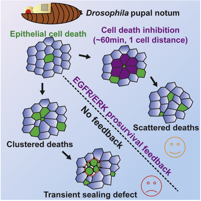
Figure 6.

Schematic of the impact of ERK pulses on cell death distribution

Schematic of the local ERK feedback (magenta) and its impact on the distribution of cell eliminations (green cells, caspase activation). Upon EGFR depletion, simultaneous caspase activations and cell eliminations can occur, which lead to aberrant extrusions and transient loss of sealing (phase outlined in yellow, white area between green aggregates) followed by wound healing.

Video S5. ERK pulses affect caspase dynamics and cell elimination, related to Figures 4 and 5

(A) Local projection of a pupal notum expressing GC3Ai (green and right, effector caspase activity) and miniCic (magenta, middle). Green circles track the nucleus of the first dying cell. Purple circles track the nucleus of a neighbor undergoing transient caspase inhibition (slow-down of GC3Ai signal increase). Scale bar, 10 μm.

(B) Local projection of a pupal notum depleted for EGFR (pnr-gal4, UAS-egfrdsRNA) expressing GC3Ai (green and right, effector caspase activity) and E-cad-tdTomato (magenta). Colored contours show neighbouring cells activating caspase. Scale bar, 10 μm.

(C) Local projection of a pupal notum depleted for EGFR (pnr-gal4, UAS-egfrdsRNA) marked with E-cad-GFP showing every cell extrusion (colored circles). Anterior, left; posterior: right. Circles appear at the termination of extrusion (orange) and stay for nine frames (progressively becoming blue). Scale bar, 10 μm.

(D) Local projection from different pupal nota depleted for EGFR (pnr-gal4, UAS-egfrdsRNA) marked with E-cad-GFP showing four examples of clusters of cell extrusion (cyan, more than four cells) followed by aberrant extrusions (relaxation, wound healing and E-cad accumulation at vertices). Scale bar, 10 μm.

Discussion

High rates of cell elimination are widespread during development and in adult tissues with high cell turnover. Similar local feedback mechanisms may be required for coherent cell elimination in the gut to prevent transient and recurrent sealing defects that could lead to chronic inflammation and inflammatory bowel disease (Blander, 2016). Importantly, the mechanism we characterized in this study is conserved in mammals, as similar ERK dynamics were observed near dying MCF10A cells, which also generate transient resistance to apoptosis (Gagliardi et al., 2021). Interestingly, other reports have also described Ca²⁺ and ERK activation waves emanating from extruding MDCK and MCF10A pre-tumoral cells or caspase-induced extrusion (Aikin et al., 2020; Takeuchi et al., 2020). However, in these cases the waves promote extrusion of the dying/extruding cells through collective convergent movements. In contrast, we still see a high rate of cell extrusion upon depletion of ERK feedback in the pupal notum (UAS-EGFR dsRNA, trametinib injection, or rolled RNAi). Strikingly, the range of the communication seems to be very different in the notum (one cell row) and in mammalian cells (3 to 15 cells from the eliminated cell), suggesting that either the relays of communication are different or that the mechanical properties of these cells are very different. Accordingly, similar ERK waves were described in the tracheal placodes of the Drosophila embryo, where the waves are propagated through a positive feedback loop between the ligand, Spitz, and its activator, Rhomboid (Ogura et al., 2018), a mechanism reminiscent of the induction of ERK in midgut stem cells near dying enterocytes, which is also driven by induction of Rhomboid (Liang et al., 2017). Altogether, this suggests that different mechanisms of propagation may alter the range and the characteristic time of ERK propagation.

In our analysis of cell death distribution, we voluntarily ignored the effects of tissue-wide patterning on the distribution of cell death and focused on local effects. While we found a clear transient dispersive effect on cell death distribution, at this stage we cannot exclude that other processes could also modify the local distribution of cell death probability (e.g., a transient and local positive feedback on caspase activity). In the long term, a better characterization of the characteristic timescale and space scale of deterministic versus self-organized regulations of apoptosis/extrusion will be essential to fully comprehend cell death distribution. Interestingly, EGFR/ERK inhibits apoptosis through Hid downregulation/inhibition (Bergmann et al., 1998; Kurada and White, 1998; Moreno et al., 2019), while Dronc activates effector caspases downstream of Hid (Fuchs and Steller, 2011). This explains how cell elimination by optoDronc can bypass the protective effect of ERK and trigger clustered eliminations.

Although, at this stage, we cannot rule out the contribution of contact-dependent communication for ERK activation in cells neighboring dying cells, evidence point to a contribution of cell stretching. First, ERK activation dynamics correlate very well with transient cell stretching (Figures 3F and 3G) and occurs very fast (a few minutes). ERK activation is also reduced upon stress release through T1 transition (Figures S5G and S5H). Moreover, we previously showed that cell stretching could promote cell survival through EGFR (Moreno et al., 2019). Accordingly, we found that EGFR depletion completely abolished ERK feedbacks near dying cells. We excluded the contribution of calcium signaling and an active secretion of the ligand from the dying cell, while laser-induced wound healing was sufficient to promote neighboring cell stretching and ERK activation. Other recent works have characterized the rapid effect of cell stretching on ERK activation (Aoki et al., 2017, 2013), which was shown to also rely on EGFR (Hino et al., 2020). Interestingly, we observed a significant decrease in ERK activation upon inhibition of EGF/Spitz in the neighboring cells (Figures S5C and S5D; Video S4C). This suggests that cell stretching could promote an autocrine activation of EGFR/ERK through enhanced EGF/Spitz release. Further work characterizing the molecular mechanism of cell deformation sensing by ERK will be required to fully test the contribution of mechanics in extrusion-induced ERK activation.

The occurrence of aberrant extrusions remarkably increases for clusters of three or more cells. However, we do not know at this stage what triggers these abnormal extrusions. On the one hand, abortive extrusion may be related to the distance that needs to be closed by the neighboring cells: while this can be short for rows of cells (using the shortest axis), it will be longer for clusters and may prevent fast fusion of neighboring cell junctions and gap closure (Staddon et al., 2018). On the other hand, abortive extrusion may be related to caspase-induced remodeling of tricellular junctions (Higashi and Chiba, 2020), which are shared by caspase-positive cells only in the case of clustered cell eliminations. Interestingly, some tricellular junction components are reportedly cleaved by caspases (Janke et al., 2019). Further characterization of extrusion dynamics will be required to test these hypotheses.

Interestingly, 2D simulations of cell disappearance combined with transient death refractory phase in the neighboring cells suggest that ERK feedback could have a significant impact on the total number of dying cells (Figure S6D). This buffering effect increases sharply with the rate of cell elimination (Figure S6D). As such, it may be essential in conditions of high stress to dampen the rate of cell elimination and prevent tissue collapse. Moreover, this feedback could be sufficient to increase the rate of cell death near clones resistant to apoptosis when they are located in regions with a high rate of cell death (Figure S6E). This suggests that extrusion-driven ERK feedback may be sufficient to recapitulate some of the features of cell competition: namely, a contact- and context-dependent increase in cell death near mutant clones (Clavería and Torres, 2016). Altogether, we propose that epithelial robustness and plasticity may be emerging features of local and transient ERK feedback driven by cell death.

Limitations of the study

As discussed above, at this stage we cannot exclude the contribution of other processes to the spatiotemporal distribution of cell death, including patterning and tissue-scale modulation of the rate of cell death, as well as very transient and local feedback loops that cannot easily be detected through our analysis. Finally, while most of our data are in agreement with a role of mechanics in ERK activation, we cannot exclude, at this stage, the contribution of other activation mechanisms that are based on contact-dependent signaling and/or short-range diffusion. Further work is required to elucidate the molecular mechanisms of ERK activation near dying cells.

STAR★Methods

Key resources table

REAGENT or RESOURCE	SOURCE	IDENTIFIER
Chemicals, peptides, and recombinant proteins
Trametinib	Santa Cruz	CAS 871700-17-3
Experimental Models: Drosophila melanogaster lines
E-cad-tdTomato (KI)	(Huang et al., 2008)	BDSC_58789
E-cad-GFP (KI)	(Huang et al., 2008)	BDSC_60584
UAS-optoDronc	This study	N/A
sqh-Sqh-3XmKate2	(Pinheiro et al., 2017)	Yohanns Bellaïche (Institut Curie, Genetics and Development, France)
Tub-miniCic-mScarlet	This study	N/A
ubi-EKARnls	(Ogura et al., 2018)	Shigeo Hayashi (CDB, Riken, Japan)
UAS-EGFR dsRNA	VDRC	KK 107130
UAS-spitz dsRNA	VDRC	GD 3922
UAS-GcAMPx20	Bloomington	BDSC_32236
UAS-GC3Ai	(Schott et al., 2017)	Magalie Suzanne (CBI, Toulouse, France)
GMR-gal4	Bloomington	BDSC_1104
UAS-his3.3 mIFP-T2A-H01	Bloomington	BDSC_64184
Hs-flp22;; Act<cd2<gal4,UAS-GFP	(Moreno et al., 2019)	(Moreno et al., 2019)
UAS-rolled dsRNA	VDRC	GD 35641
ubi-Dlg-mRFP	(Pinheiro et al., 2017)	Yohanns Bellaïche (Institut Curie, Genetics and Development, France)
UAS-Cd4-mIFP-T2A-H01	Bloomington	BDSC_64182
Oligonucleotides
GFPlinkerF: TTATAGCGGCCGCATGTCCAAAGGTGAAGAACT	This study	N/A
GFPlinkerR: AATTTCTAGAAGATCTGCCGCCTCCT CCGGACCCACCACCTCCAGAGCCACCGCCACC CTTGTAGAGCTCATCCATGCCGT	This study	N/A
Dronc-linkerF: AATTAGATCTATGCAGCCGCCGGAGCTCGAGATT	This study	N/A
Dronc-linkerR: AATTTCTAGAGCTAGCGCCGCCTCCTCCGGACCC ACCACCTCCAGAGCCACCGCCACCTTCGTTGAAA AACCCGGGATTG	This study	N/A
CRY2PHR-F: AATTAGATCTATGCAGCCGCCGGAGCTCGAGATT	This study	N/A
CRY2PHR-R: AATTTCTAGACTATGCTGCTCCGATCATGATCTGT	This study	N/A
miniCiclinkerF: GTGAAGGTACCCGCCCGGGGATCAGATCC	This study	N/A
miniCiclinkerR : ACAGAACCACCACCAGAACCAC	This study	N/A
mScarletF : CGGTGGTGGTTCTGGTGGTGGTTCTGTGAGCAA GGGCGAGGCA	This study	N/A
mScarletR : CAGAAGTAAGGTTCCTTCACAAAGATCCTCTAG ATTACTTGTACAGCTCGTCCATGC	This study	N/A
Recombinant DNA
pCaSperR4-tubp-Gal80 plasmid	Addgene	RRID: Addgene_17748
pJFRC4-3XUAS-IVS-mCD8::GFP plasmid	Addgene	RRID : Addgene_26217
pJFRC19-13XLexAop2-IVS-myr::GFP plasmid	Addgene	RRID : Addgene_26224
Dronc gold cDNA	DGRC	LP09975, RRID : FBcl0184379
pGal4BD-CRY2	Addgene	RRID : Addgene_28243
Software and algorithms
Matlab with Image processing toolbox and Statistics and Machine learning toolbox	https://fr.mathworks.com/	N/A
Fiji (ImageJ)	https://fiji.sc/	N/A
Black Zen Software	Zeiss	RRID: SCR_01863
Mypic Zen autofocus macro	https://git.embl.de/grp-ellenberg/mypic	N/A
Adaptive local z-projection macro (Matlab)	Code published in the associated reference	(Moreno et al., 2019)
Local z-projector plugin (Fiji)	https://gitlab.pasteur.fr/iah-public/localzprojector	(Herbert et al., 2021)
Graphpad Prism8	https://www.graphpad.com/	N/A
Packing analyser (now tissue miner in Fiji)	https://github.com/mpicbg-scicomp/tissue_miner/blob/master/MovieProcessing.md	(Etournay et al., 2016)
Epyseg	https://github.com/baigouy/EPySeg	(Aigouy et al., 2020)
Python 3.7	http://www.python.org	RRID: SCR_008394
Raw data and codes
Raw data and codes for simulation (python)	This study	http://doi.org/10.5281/zenodo.4593444

Resource availability

Lead contact

Further information and requests for resources and reagents should be directed to and will be fulfilled by the lead contact, Romain Levayer (romain.levayer@pasteur.fr).

Material availability

All the reagents generated in this study will be shared upon request to the lead contact without any restrictions.

Data and code availability

All code generated in this study and the raw data corresponding to each figure panel (including images and local projection of movies) can be found in the following repository: http://doi.org/10.5281/zenodo.4593444. Further information about the dataset can be requested to the lead contact.

Experimental model and subject details

Drosophila melanogaster maintenance and strains

All the experiments were performed with Drosophila melanogaster fly lines with regular husbandry technics. The fly food used contains agar agar (7.6 g/l), saccharose (53 g/l) dry yeast (48 g/l), maize flour (38.4 g/l), propionic acid (3.8 ml/l), Nipagin 10% (23.9 ml/l) all mixed in one liter of distilled water. Flies were raised at 25°C in plastic vials with a 12h/12h dark light cycle at 60% of moisture unless specified in the legends and in the table below (alternatively raised at 18°C or 29°C). Both females and males were used without distinction for all the experiments, as no obvious differences were found between sexes. We did not determine the health/immune status of pupae, adults, embryos and larvae, they were not involved in previous procedures, and they were all drug and test naïve.

The following fly lines were used in this study: E-cad-tdTomato (KI) (II, (Huang et al., 2008), BDSC_58789), E-cad-GFP (KI) (II (Huang et al., 2008), BDSC_60584), UAS-optoDronc (II, this study), sqh-Sqh-3XmKate2 (II (Pinheiro et al., 2017), gift from Yohanns Bellaïches, Institut Curie, France), Tub-miniCic-mScarlet (II, this study), ubi-EKARnls (II (Ogura et al., 2018), gift of Shigeo Hayashi, CDB, Riken, Japan), UAS-EGFR dsRNA (II, VDRC, KK 107130), UAS-spitz dsRNA (II, VDRC, GD 3922), UAS-GcAMPx20 (III, Bloomington, BDSC_32236), UAS-GC3Ai (III (Schott et al., 2017), gift from Magalie Suzanne, CBI, Toulouse, France), GMR-gal4 (II, Bloomington, BDSC_1104), UAS-his3.3 mIFP-T2A-H01 (III, Bloomington, BDSC_64184), Hs-flp22;; Act<cd2<gal4,UAS-GFP (I, III (Moreno et al., 2019)), UAS-rolled dsRNA (II, VDRC, GD 35641), ubi-Dlg-mRFP (I (Pinheiro et al., 2017), gift from Yohanns Bellaïche, Institut Curie, France), UAS-Cd4-mIFP-T2A-H01 (III, Bloomington, BDSC_64182).

The exact genotype used for each experiment can be found in Table S1.

Method details

Design of optoDronc

The GFP-linker-DRONC-linker-CRY2PHR was first cloned in the pCaspeR4-Tubp-Gal80 vector (addgene 17748) and subsequently cloned in the pJFRC4-3XUAS-IVS-mCD8::GFP (Addgene 26217). Initial cloning was performed by three successive amplifications/ligations. Briefly, GFP was first inserted in pCaspeR4-Tubp by PCR-amplifying GFP from pJFRC19-13XLexAop2-IVS-myr::GFP (Addgene 26224) adding NotI, BglII, XbaI restriction sites and linkers, and eventually ligation into pCasper4-TubP-Gal80 after digestion with NotI and XbaI. Dronc cDNA was then inserted in this plasmid through PCR amplification on the cDNA clone LP09975 (DGRC) adding BglII, NheI and XbaI restriction sites and linkers, and then ligation into pCasper4-TubP-GFP-linker cut with BglII and XbaI. Finally, CRY2PHR was inserted by amplifying residues 1-498 of CRY2 from pGal4BD-CRY2 (Addgene 28243) while adding NheI and XbaI sites and ligation into pCasper4-TubP-GFP-linker-DRONC-linker cut with NheI and XbaI. The GFP-linker-Dronc-linker-CRY2PHR was cut with NotI and XbaI and inserted by ligation in pJFRC4-3XUAS-IVS-mCD8::GFP (Addgene 26217) after digestion with NotI and XbaI. The construct was checked by sequencing and inserted at the attp site attp40A after injection by Bestgene. The details about the primers used for this construct can be found in the key resources table.

Induction of cell death using optoDronc

To induce optoDronc in the eye, GMR-gal4 females were crossed with homozygous males UAS-optoDronc. Tubes containing crosses and progeny were either kept in the dark at 25°C (control) or maintained in a cardboard box permanently lighted by a blue LED array (LIU470A, Thorlab) in the same 25° incubator as the control. Female adult eyes were then imaged on a Zeiss stereoV8 binocular equipped with a colour camera (Axiocam Icc5).

For induction of optoDronc in clones in the pupal notum, hs-flp; E-cad-tdTomato(KI); act<cd2<G4 females were crossed with homozygous UAS-optoDronc or UAS-optoDronc; UAS-p35. Clones were induced through a 12 minutes heat shock in a 37°C waterbath. Tubes were then maintained in the dark at 25°C. White pupae were collected 48 hours after clone induction and aged for 24h at 25°C in the dark. Collection of pupae and dissection were performed on a binocular with LED covered with home-made red filter (Lee colour filter set, primary red) after checking that blue light was effectively cut (using a spectrometer). Pupae were then imaged on a spinning disc confocal (Gataca system). The full tissue was exposed to blue light using the diode 488 of the spinning disc system (12% AOTF, 200ms exposure per plane, 1 stack/min). The proportion of remaining cells was calculated by measuring the proportion of cells remaining in the tissue at time t compared to t0. Extrusion profiles were obtained by segmenting extruding cells in the optoDronc clones with E-cad-tdTomato signal (only single cell clones in this case) or WT cells marked with E-cad-GFP in the posterior region of the notum using Packing analyser (Etournay et al., 2016). Curves were aligned on the termination of extrusion (no more apical area visible) and normalised with the averaged area on the first five points. Clone area profile (Figures 1D and 5I) were obtained by segmenting the group of cells in the clone and calculating the area and the solidity (Area/Convex Area) on Matlab. Categorisation of normal versus abnormal extrusion was based on the dynamics of clone contraction: transient relaxation or accumulation of E-cad at vertices was counted as abnormal extrusion. Large relaxation combined with clear E-cad accumulation at vertices was counted as “transient holes”.

Design of miniCic-mScarlet

The pCaspeR4-Tubp-miniCic-linker-mScarlet-I was obtained by amplifying by PCR miniCic-linker from pCaspeR4-Tubp-miniCic-linker-mCherry(Moreno et al., 2019) and mScarlet-I from pmScarlet-i_C1 (Addgene 85044). These two inserts were cloned in the vector pCaspeR4-TubP-Gal80 linearised by NotI, XbaI digestion (to excise Gal80) using NEBuilder HiFi DNA Assembly Method. The construct was checked by sequencing and inserted through P-element after injection by Bestgene. Details about the primers used for this construct can be found in the key resources table.

The construct was tested by comparing the dynamics and pattern in the notum compared to previously characterised dynamics using miniCic-mCherry (Moreno et al., 2019). Similar dynamics were also observed at the single cell level between miniCic-mScarlet and the FRET sensor ubi-EKARnls (Ogura et al., 2018) (Figure S4).

Live imaging and movie preparation

Notum live imaging was performed as followed: the pupae were collected at the white stage (0 hour after pupal formation), aged at 29°, glued on double sided tape on a slide and surrounded by two home-made steel spacers (thickness: 0.64 mm, width 20x20mm). The pupal case was opened up to the abdomen using forceps and mounted with a 20x40mm #1.5 coverslip where we buttered halocarbon oil 10S. The coverslip was then attached to spacers and the slide with two pieces of tape. Pupae were collected 48 or 72h after clone induction and dissected usually at 16 to 18 hours APF (after pupal formation). The time of imaging for each experiment is provided in Table S1. Pupae were dissected and imaged on a confocal spinning disc microscope (Gataca systems) with a 40X oil objective (Nikon plan fluor, N.A. 1.30) or 100X oil objective (Nikon plan fluor A N.A. 1.30) or a LSM880 equipped with a fast Airyscan using an oil 40X objective (N.A. 1.3), Z-stacks (1 μm/slice), every 5min or 1min using autofocus at 25°C. The autofocus was performed using E-cad-GFP plane as a reference (using a Zen Macro developed by Jan Ellenberg laboratory, MyPic) or a custom made Metamorph journal on the spinning disc. Movies were performed in the nota close to the scutellum region containing the midline and the aDC and pDC macrochaetae. Movies shown are adaptive local Z-projections. Briefly, E-cad plane was used as a reference to locate the plane of interest on sub windows (using the maximum in Z of average intensity or the maximum of the standard deviation). Nuclear signal was then obtained by projecting maximum of intensity on 7 μm (7 slides) around a focal point which was located 6 μm basal to adherens junctions. This procedure was either applied using a custom Matlab routine (Moreno et al., 2019) or through the Fiji plugin LocalZprojector (Herbert et al., 2021).

Laser ablation

Photo-ablation experiments were performed using a pulsed UV-laser (355nm, Teem photonics, 20kHz, peak power 0.7kW) coupled to a Ilas-pulse module (Gataca-systems) attached to our spinning disk microscope. The module was first calibrated and then set to 40-60% laser power. Images were taken every 500ms and 3 to 6 single cells were ablated 10 images after the beginning of the movie (20 repetitions of “point” ablation ∼50ms exposure per cell). Cells were selected in regions with high and homogeneous nuclear miniCic levels. For each single cell ablation, miniCic signals over time were extracted in 4 cell nuclei of the first row and second row of cells around the ablated cell. Nuclei were visualized and clicked by hand using the Histone3-mIFP fluorescent channel after a local z-projection. Background value for each movies (for miniCic) were extracted and removed from the signals, then the single cell miniCic signal was normalized to 1 using the first 5 time points.

Dextran and drug injection in pupal notum

30 h APF pupae were glued on double sided tape and the notum was dissected with red filter. Pupae were then injected using home-made needles (borosilicate glass capillary, outer diameter 1 mm, internal diameter 0.5 mm, 10 cm long, Sutter instruments) pulled with a Sutter instrument P1000 pipette pulling apparatus. Dextran Alexa 647 10,000 MW (Thermofisher, D22914) was injected at 2 mg/ml in the thorax of the pupae using a Narishige IM400 injector using a constant pressure differential (continuous leakage) and depressurisation in between pupae. Imaging of Dextran leakage in live pupae was performed after local projection using E-cad plane as a reference to measure Dextran concentration at the junction plane (note that septate junctions are located basally to adherens junctions). Dextran intensity was measured using a ROI in the center of the clone after normalization using the first 5 time points and removal of intensity background (estimated on a region with no signal). Note that Dextran injection cannot be used to track leakages over long time scales (>4 hours) as the majority of Dextran get rapidly trapped in fat body cells and in epithelial cell endosomes.

Injection of Trametinib (Santa Cruz) was performed with a stock solution in DMSO at 10 mM, after a dilution by 10 in water. The control was obtained with the injection of DMSO diluted 10 folds. ERK dynamics was analysed once we observed a global inhibition of ERK throughout the tissue (2–3 h after injection).

Signaling dynamics and cross-correlation

Measurement of ERK activity

ERK dynamics were measured using the mean nuclear intensity of miniCic. Whenever possible, a marker of the nucleus (His3-mIFP) was used to track the nucleus manually (Fiji macro). EKAR FRET signal was obtained after local projection on 6 planes of CFP and YFP signals. CFP and YFP signals were blurred (Gaussian blur, 2 pixel width) and the ratio of YFP/CFP signal was then calculated. Raw YFP-nls signal was thresholded and used as a mask to only keep nuclear FRET signal. For the comparison of miniCic and EKAR, single curves from the same cell were aligned on the peak of the FRET signal (maximum value) and eventually averaged for all the cells.

For the measurement of miniCic in neighbours combined with apical area (Figure 3), cell contours were tracked using E-cad-GFP (Packing analyser), while nuclei were manually tracked on Matlab using His3-mIFP. For each dying cell, the nuclear miniCic intensity and apical area were measured in the neighbours (first and second rows), aligned on the termination of extrusion (area=0), normalised using 5 times points around -50 min and averaged.

Analysis of GC3Ai signal

To analyse caspase activity, we used the differential of GC3Ai signal as a proxy. GC3Ai becomes fluorescent upon cleavage of a domain by effector caspases which triggers GFP folding and maturation (Schott et al., 2017). The dynamics of GFP signal can be written as follows:

$$\frac{dG}{dt}=C.G_0-\alpha .G$$

Where G stands for concentration of active GFP, C concentration of active effector caspase, G₀ concentration of inactive GFP, and α rate of GFP degradation.

On timescales of one hour, we can neglect GFP degradation. Assuming a constant pool of inactive GC3Ai, G₀ can be considered as a constant. As such:

$$\frac{dG}{dt}=C.G_0$$

Therefore the change of intensity over time should be proportional to effector caspase activity (C).

To analyse the dynamics of caspase activity in cells neigbouring extruding cells, movies were segmented using E-cad-tdTomato signal and Tissue Analyser plugin on ImageJ (Aigouy et al., 2010). Cells and bonds data were then imported, tracked and analysed in a homemade Matlab script. The segmentation results and tracks were used to measure the GC3AI signal in every cell. First the signal was smoothed using Matlab smooth function (rolling mean on 8 time points) to reduce noise. Then we used its derivative $\frac{dGC3AI}{dt}$ as a proxy for caspase 3 activity at time t and smoothed it again (Matlab rolling mean on 5 time points).

We wanted to detect cell activating caspase (‘on’ state). To avoid detection of false positive cells due to fluctuation in GC3AI signal we set 2 criteria which define a cell state as ‘on’: i) a threshold signal T = 2 x σ_c (with σ_c the standard deviation of GC3Ai differential signal in “negative” cells), ii) which has to last at least for 3 consecutive time points (Δt ≥15 min).To ensure robustness of those criteria we also performed a parameter sweep for different values of T and Δt.

We then checked cell state of cells neighbouring extruding cells in a time window $\Delta t\pm 30min$ around extrusion. Neighbouring cells were detected as sharing bounds and vertices with extruding cells. 87 extruding cells were analysed which represent 359 neighbours. The probability of a cell to have 1 or more neighbours ‘on’ has been calculated as such:

$$p=\sum _{i=1}^6\frac{N_{ext,i}}{N_{ext,total}}$$

Where N_ext,i is the number of extruding cells having i neighbours caspase positive and N_ext,total the total number of extruding cells (87).

For the analysis of GC3Ai signal dynamics, we used movies of GC3Ai from local projection (using E-cad or nuclear miniCic as a reference) and measurement of mean intensity on small circular ROI at the center of the cell (Fiji). The differential was calculated using the Diff function of Matlab after smoothing the intensity curve (50 minutes averaging window) and aligning the curves on the time of the first cell disappearance (apical area=0, end of extrusion). Note that the analysis of caspase dynamics was restricted to neighbours having a positive slope before the elimination of the first cell (in order to see caspase shutdown). The reference cell was defined as the one extruding the first.

To cross-correlate GC3Ai and ERK dynamics, local projections centered on nuclear miniCic were used (with GC3Ai plane of interest shifted apically). miniCic nuclear intensity and GC3Ai cytoplasmic intensity were measured by manually tracking small circular ROI (20 pixels diameter) in the center of the cells (Fiji home-made macro). The cross-correlation between GC3Ai differential and miniCic nuclear signal was calculated on Matlab with the xcorr function with the ‘coef’ option (normalised cross-correlation). All the curves (one per cell) were then averaged.

Measurement of GCaMP

GCaMP signal was measured on local projections using E-cad-tdTomato as a reference plane after global correction for bleaching. Each cell extrusion was cropped and the movie realigned using the Stackreg Fiji plugin. GCaMP signal was then measured using the mean intensity in a 20x20 pixel square in the center of each cells. Each single cell curve was aligned (time 0 at the termination of extrusion) and normalised using 5 time values around time 0.

Statistical analysis of cell death distribution

Calculation of the probability to observe three cells clustered elimination

We wanted to evaluate the probability to observe a cluster of three cells eliminated in less than 30 minutes.

We first considered a hexagonal grid of points in a squared array (N cells per side) and assumed periodic boundaries. The probability of single cell disappearance over 30 min is p. As such the probability to observe a specific cluster of 3 cells eliminated in the same 30 min window is p³. The total number of possible 3 cells configurations is approximatively given by: $2.N^2$ (number of independent triangles of 3 cells we can obtain on an hexagonal grid). Using the posterior region of WT nota, we estimate p∼0.04 (probability of cell elimination in 30 minutes). As such for a group of 800 cells (covering the full posterior region with high death rate) observed for 20 hours (T= 40 times 30 minutes), the expected number of 3 cell-cluster elimination is given by: $E\left(numberofclusters\right)=2N^2{p}^{3}T\cong$ 4.1.

Second, we took the experimental death characteristics (total area of the region analysed and death rate) from the 5 WT and 4 EGFR RNAi experiments and simulated spatiotemporal distribution of death for movies of 20h assuming a Poisson process. We used areas of simulation two times bigger than the one used in the death density analysis (Figure 2), which corresponds to the area used for cluster characterisation in experiments (Figure 5G). We then compute the number of group of 3 deaths or more happening within 30 minutes periods and within distances of 8 and 12 μm respectively (to take into account differences in cell size between WT and EGFR RNAi). For each experimental movie and the corresponding death rate, we performed 200 simulations and obtained one mean value (= one dot in Figure 5G).

Therefore, we would expect to observe several occurrences of 3 cell-cluster eliminations per movie.

Analysis of death distribution

For the analysis of death distribution we selected movies lasting 16 to 20 hours in the posterior region of the pupal notum. Cell extrusion events were clicked by hand and checked twice. Extrusion localisations were corrected for global drift (translation) of the tissue (Matlab procedure). Spatio-temporal distribution of deaths was first checked by x-y-t histogram. According to that distribution, for each movie, an area of interest (in time and space) was selected by hand to obtain an area where distribution was as homogeneous as possible (double checked by x-y-t histograms). These data sets were then the basis of three statistical analyses (see below).

Distribution of distances

Distances in time and space between all couples of extrusions were computed. For each data set we plotted the maps of densities of death at a given distance (number of deaths divided by the area of the disc considered) as a function of spatial and temporal distances from each dying cell. From each data set we estimated the effective death rate, i.e. the intensity of the random spatio-temporal process, and used it to simulate the corresponding Poisson process 200 times. For each simulation we performed the same analysis as for the experimental data set, namely calculating maps of death densities, and eventually averaged the 200 maps. Finally, for each movie we calculated the difference between the averaged simulated map and the corresponding experimental map. We show in the main figures the average of the “difference map” for every experiment (5 for WT, 4 for EGFR-RNAi). Due to the very small amount of death occurrence for very short distance (<2 micrometers, half of a cell size) and the associated short area, these local densities showed very high variability in the simulations (up to 4 times the mean values). We therefore excluded these distances from the analysis and only represented maps from 2 to 25 um and from 0 to 150 min. The apparent proximo-distal gradient is driven by border effects: for large radius search, a significant amount of area is outside the death search window, hence reducing the number of deaths events per unit of space. This explains the apparent low densities at high distance both in experiments and simulations. This bias is however similar in experiments and simulations and does not affect the characterization of the differences between experimental and simulated distributions.

Closest neighbour analysis

For each death event, we calculated the Euclidean distance to the closest death in a given time window. Based on the previous analysis, we selected windows of 20’ to 1h20’, 1h20’ to 2h20’ and 2h20’ to 3h20’. We excluded the first 20 minutes as they correspond to the characteristic time of extrusion (where cells cannot be reverted anymore). We then ordered these shortest distances by size and plotted the cumulative probability of closest death at a given distance. A value of 40% at a distance of 10 micrometers means than 40% of the closest deaths are localized between 0 and 10 micrometers away. Similar analysis were run on simulations of a Poisson process with the same death rate without or with a negative feedback (5 μm range, 60 min).

For the analytic calculation of the cumulative probability of a Poisson process, we consider p, the probability of death of one cell inside a time window of T minutes, given by:

$$p=1-e^{-{\lambda }_{d}T}$$

where λ_d is the intrinsic rate of death per minute. In a disk of a radius x there is approximately cx² cells. As such, the cumulative probability function that there is no death on a distance x from the extruded cell is 1 − (1 − p)^cx2 which can be developed in:

$$F\left(x\right)=1-e^{-{\lambda }_{d}Tc{x}^2}$$

Using a continuous approximation of the process, the cumulative probability can be expressed as:

$$F\left(x\right)=1-e^{-{\lambda }_c\pi Tx}$$

where λ_c is an intrinsic rate of death per minute and per unit of surface (μm²), T the time window and x, distance in μm. Note that ${\lambda }_c\text{π}=c{\lambda }_d$, as such: ${\lambda }_d=\frac{{\lambda }_c\pi }{c}$.

p-values test using “K-functions” and random labeling test

This procedure is used for estimating how far is one spatio-temporal process from a purely random Poisson process (Smith, 2020). The test is performed in two main steps. The first step consists of calculating so-called "K-functions" of the given process, and the second is the random re-labeling test as explained below.

The space-time K-function of the observed process, $K^0\left(r,h\right)$, is defined as the expected number of additional events within the space-time distance $\left(r,h\right)$ of a randomly selected event. It depends on the intensity $\lambda$ of the spatio-temporal process and it can be estimated using only the observed events and without additional assumption on the process.

The complete absence of dispersion or clustering in a given process implies that there is no relation between the location and timing of events. This is formally given through the temporal indistinguishability hypothesis. Under this hypothesis, there is an equal probability to observe our set of events, or events with the same locations in space but with shuffled times. From here we can perform the random labeling test as follows.

We draw a sample of $N$ random permutations of the times of events. For a given space-time distance $\left(r,h\right)$ we calculate the value of the K-function, $K\left(r,h\right)$, for each permutation. We compute the number $M\left(r,h\right)$ of sampled re-labelings with the value of the K-function smaller than the one of the original labeling, i.e. $K\left(r,h\right)<K^0\left(r,h\right)$. Then, the probability of obtaining a value as small as $K^0\left(r,h\right)$ is estimated by the space-time dispersion p-value: $p\left(r,h\right)=\left(M\left(r,h\right)+1\right)/\left(N+1\right)$. If we repeat the same procedure for all space-time distances $\left(r,h\right)$, we obtain the map of dispersion p-values.

This procedure is implemented in Python. The maximum distance is set to $r_{max}=25\mu m$, and the maximum temporal interval to $h_{max}=150\min$. We subdivided these maximum values in 25 and 30 equal increments ($1\text{μ}\text{m}$ and $5\min$). We simulated 9999 re-labellings of times to test for space-time dispersion of the extrusion events. The results of these 750 tests are plotted on a grid and then interpolated to obtain a p-value map. We performed this procedure for each movie.

Single cell death analysis

This pipeline is used to define the probability of death for the first versus second row of cells around a dying cell, in the following 0 h 20 min to 1 h 20 min and 1 h 20 min to 2 h 20 min time periods.

First, a sub-area of the movie is duplicated to keep only the space location and timings used in the others spatiotemporal analysis of death distribution. Second, the movies of E-Cad signal is pre-treated with the machine learning based Epyseg software (Aigouy et al., 2020) to improve cell-cell junctions contrast using a pre-trained model. Images where then imported to Tissue Analyser FiJi plugin (Etournay et al., 2016). Segmentation is performed on improved images then corrected by hand for the remaining segmentation errors. Death were then automatically tracked using the “track dying cell” option, while not keeping cell deaths at the image borders. Cells identities and boundaries over time were as well extracted from Tissue Analyzer as excel files and imported to Matlab. From the identity (in space and time) of the dying cell, we recover the identities of the cells at one and two cells distances 20 minutes before it dies. We then quantify when these cells die. From these quantifications we calculate the probability of death for row 1 and row 2 during 0 h 20 min-1 h 20 min and 1 h 20 min-2 h 20 min time periods after the death of the central cell as well as the 95% confidence interval. The 95% confidence interval around the mean value for these binary variables (alive=0, dead=1) was calculated as 1.96$\frac{\sqrt{m_v(1-m_v)}}{\sqrt{n}}$ where $m_v$ is the death probability and n the total number of neighbouring cells in row 1 or row 2. We applied this routine to two WT and two EGFR RNAi movies.

Calculation of the effective death rate with caspase resistant neighbours

We assume that the cell has six neighbours, and $n$ neighbours resistant to apoptosis ($n\le 6$), and that the death of one neighbour will protect the cell for a period $T$. The probability of a cell to die at the time $t$ is the probability that none of its $(6-n)$ sensitive neighbours died during the period $T$ prior to $t$, multiplied by its intrinsic probability to die at the moment $t$. The death of each isolated sensitive cell is a random event modelled as a temporal Poisson process, with the event rate $\lambda$ (expected number of cell deaths per minutes).

By definition, for the Poisson process $X$ with rate $\lambda$ the probability of the event (death) to happen in the time interval $[t,t+dt]$, for $dt$ very small, is:

$$P\left\{X\in [t,t+dt]\right\}=\lambda e^{-\lambda t}dt.$$

From here, the probability that an isolated sensitive cell dies during a time period of length $T$ is:

$$P\left\{X\in [0,T]\right\}={\int }_0^T\lambda e^{-\lambda t}dt=1-e^{-\lambda T},$$

and the probability that it does not die during this time is: $1-(1-e^{-\lambda T})=e^{-\lambda T}.$

The probability that the cell dies in a given moment $t$ is defined as the probability to die in the time interval $[t,t+dt]$, for $dt$ very small, under assumption that it didn't die until the time $t$. It is the same as the probability that it dies in the time interval $[0,dt]$:

$$p:P\left\{X\in [t,t+dt]|X\notin (0,t)\right\}=P\left\{X\in [0,dt]\right\}=\lambda e^{-\lambda 0}dt=\lambda dt.$$

This is also one of the definitions for the rate of the temporal Poisson process.

Thus, for the cell with six neighbours, where $n$ neighbours are resistant to apoptosis ($n\le 6$), the probability to die at the given moment $t$ is:

$$p_e=\lambda e^{-{\lambda }_{e}T(6-n)}dt={\lambda }_{e}dt.$$

Here we approximated the self-inhibiting random process with a Poisson process with a different death rate, that we name the effective rate of death, and we used this rate to express the probability that the neighbouring cells do not die during the period $T$. Finally, the effective rate is:

$${\lambda }_e=\frac{L_W\left(\lambda T(6-n)\right)}{T(6-n)},$$

where $L_W$ is Lambert W function. Note that we neglect here the effect of the delay of inhibition on the neighbours. We used this expression in Figure S6E.

Calculation of the intrinsic death intensity with continuous time and space

Assume that $X$ is the spatio-temporal Poisson process. Then, by definition, the probability that the number of events that fall in the spatial region $C$ during the time period $[0,t]$ is equal to $k$, is:

$$P\{N\left(\left[0,t\right]\times C\right)=k\}=\frac{{\left(\lambda \cdot t\cdot a\left(C\right)\right)}^k}{k!}{e}^{-\lambda ta\left(C\right)},k=\mathrm{0,1,2,3\dots }$$

where $\lambda$ is the space-time intensity of the process, i.e. it is the expected number of events per unit of space-time volume (expected number of deaths per minute per micrometer squared), and $a\left(C\right)$ is the surface of the given region $C$.

Hence, the probability that no event $(k=0)$ happens on a given region $C$ during a period of time $\tau$ is: $e^{-\lambda \tau a\left(C\right)}$. If the region $C$ is a disk of radius $r$, its surface is $r^2\pi$, and this probability is: $e^{-\lambda \tau r^2\pi }$.

By definition of the space-time intensity of the process, the probability that the event happens in a given moment $t$ and that it falls on a position $(x,y)$, is given by:

$$p=\lambda dtdxdy.$$

Now we consider the self-inhibiting spatio-temporal process. Meaning, for each event there is a feedback that inhibits the process on a disk around the event of radius $r$, and during a period of time $\tau$. Such a self-inhibiting process is not anymore a Poisson process, however it can be approximated as one with a different effective intensity, ${\lambda }_e$. The probability that the death happens at some time $t$ and on a given location $(x,y)$, is the probability that there was no event in its spatio-temporal vicinity (characterised by the spatio-temporal volume of the feedback), multiplied with the probability of an isolated cell death at this moment and place, or

$$p_e=\lambda e^{-{\lambda }_e\tau r^2\pi }dtdxdy={\lambda }_{e}dtdxdy.$$

Then the observed or effective intensity, ${\lambda }_e$, can be obtained by solving the equation:

$${\lambda }_e=\lambda e^{-{\lambda }_e\tau r^2\pi }.$$

Finally,

$${\lambda }_e=\frac{L_W\left(\lambda \tau r^2\pi \right)}{\tau r^2\pi },$$

where $L_W$ is Lambert $W$ function. We can also obtain an expression for the intrinsic intensity:

$$\lambda ={\lambda }_e{e}^{{\lambda }_e\tau r^2\pi }.$$

Note that with this approximation we neglected an effect of the delay in the feedback.

This means that if we can estimate parameters of the feedback $\tau$ and $r$, and using the observed intensity, ${\lambda }_e$, we can have an estimate on the intrinsic intensity of the spatio-temporal self-inhibiting process.

To verify this expression numerically, we perform the following test: assume we want to observe an effective intensity of the process ${\lambda }_e=5.14\cdot {10}^{-5}{\min }^{-1}{\mathrm{m}}^{-2}$ with the self-inhibiting process whose feedback has the parameters: $\tau =40\min$, $r=5\text{μ}\text{m}$, and delay $10\min$. We first calculate, using the above expression the intrinsic rate of the process to be $\lambda =6.04\cdot {10}^{-5}{\min }^{-1}{\mathrm{m}}^{-2}$. Using this rate and given parameters of the feedback, we run a long simulation ($2\cdot {10}^6\min$) of the self-inhibiting process. We observed the effective intensity of this process to be: ${\lambda }_e=5.12\cdot {10}^{-5}{\min }^{-1}{\mathrm{m}}^{-2}$. For the comparison, we run the same length of the simulation of the actual Poisson process (without feedback) with the intensity $\lambda ={\lambda }_e=5.14\cdot {10}^{-5}{\min }^{-1}{\mathrm{m}}^{-2}$. The observed intensity of this simulated process is $\text{λ}=5.13\cdot {10}^{-5}{\min }^{-1}{\mathrm{m}}^{-2}$. This confirms that we have a good approximation for expression of the intrinsic intensity of the self-inhibiting process. We performed such comparisons for several values of intrinsic intensity.

We use this expression to estimate an intrinsic intensity of the processes of the experimental data, and for the simulations of self-inhibiting processes that correspond to our experiments (Figure 2H)

2D simulations of death rate

To evaluate the effect of the duration of the feedback as a function of the intrinsic rate of death we made Python routine as follows:

We use a hexagonal grid as an approximation of the cell arrangement in the tissue. Each node in the grid represents a cell, with the intrinsic rate of death $\lambda$. Number of cells per side is $n$, so in total we have $n^2$ cells. The cells can be in 2 different states: “regular” (sensitive to death), or “inhibited for death” (probability to die is 0). When one cell dies it inhibits itself, and its 6 neighbours to die during some time $T$ (in minutes).

Each death, $e=(t_e,x_e,y_e)$, is described with the time of death, $t_e$, and its coordinates in the grid $(x_e,y_e)$. We simulate the times of death for the Poisson process with rate $l=\lambda \cdot n^2$. For each simulated time, $t_e$, we assign a random position $(x_e,y_e)$ in the grid. Then we check if any of its neighbours, or itself, has died in the previous $T$ minutes. If there was no death recorded in its neighbourhood, the cell is a regular cell and we record a new death event $(t_e,x_e,y_e)$. If there was a death in its neighbourhood in the last $T$ minutes the cell is refractory to death and we do not record this event.

At the end of simulation we compute the effective death rate as ${\lambda }_e=\frac{N}{(T_{max}\cdot n^2)}$, where $N$ is a total number of recorded deaths and $T_{max}$ is the simulation time.

The parameters that we used in our simulations are the following: $n=25$ (625 cells), $T_{max}=5000\min$. We simulated effects of different inhibition times $T\in \left[\mathrm{0,5,10,20},\mathrm{\dots },150\right]\min$ with different intrinsic death rates, and repeated it 5 times per value. (Figure S6D)

Quantifications and Statistical analysis

Data were not analysed blindly. No specific method was used to predetermine the number of samples. The definition of n and the number of samples is given in each figure legend and in the table of the Experimental model section. Error bars are standard error of the mean (s.e.m.). p-values are calculated through t-test if the data passed normality test (Shapiro-Wilk test), or Mann-Whitney test/Rank sum test if the distribution was not normal. Statistical tests were performed on Graphpad Prism 8 or Matlab.

Published: June 2, 2021

References

- Aigouy B., Farhadifar R., Staple D.B., Sagner A., Röper J.C., Jülicher F., Eaton S. Cell flow reorients the axis of planar polarity in the wing epithelium of Drosophila. Cell. 2010;142:773–786. doi: 10.1016/j.cell.2010.07.042. [DOI] [PubMed] [Google Scholar]
- Aigouy B., Cortes C., Liu S., Prud’Homme B. EPySeg: a coding-free solution for automated segmentation of epithelia using deep learning. Development. 2020;147:dev194589. doi: 10.1242/dev.194589. [DOI] [PMC free article] [PubMed] [Google Scholar]
- Aikin T.J., Peterson A.F., Pokrass M.J., Clark H.R., Regot S. MAPK activity dynamics regulate non-cell autonomous effects of oncogene expression. eLife. 2020;9 doi: 10.7554/eLife.60541. [DOI] [PMC free article] [PubMed] [Google Scholar]
- Aoki K., Kondo Y., Naoki H., Hiratsuka T., Itoh R.E., Matsuda M. Propagating wave of ERK activation orients collective cell migration. Dev. Cell. 2017;43:305–317.e5. doi: 10.1016/j.devcel.2017.10.016. [DOI] [PubMed] [Google Scholar]
- Aoki K., Kumagai Y., Sakurai A., Komatsu N., Fujita Y., Shionyu C., Matsuda M. Stochastic ERK activation induced by noise and cell-to-cell propagation regulates cell density-dependent proliferation. Mol. Cell. 2013;52:529–540. doi: 10.1016/j.molcel.2013.09.015. [DOI] [PubMed] [Google Scholar]
- Bergmann A., Agapite J., McCall K., Steller H. The Drosophila gene hid is a direct molecular target of Ras-dependent survival signaling. Cell. 1998;95:331–341. doi: 10.1016/s0092-8674(00)81765-1. [DOI] [PubMed] [Google Scholar]
- Blander J.M. Death in the intestinal epithelium-basic biology and implications for inflammatory bowel disease. FEBS Journal. 2016;283:2720–2730. doi: 10.1111/febs.13771. [DOI] [PMC free article] [PubMed] [Google Scholar]
- Clavería C., Torres M. Cell competition: mechanisms and physiological roles. Annu. Rev. Cell Dev. Biol. 2016;32:411–439. doi: 10.1146/annurev-cellbio-111315-125142. [DOI] [PubMed] [Google Scholar]
- Eisenhoffer G.T., Loftus P.D., Yoshigi M., Otsuna H., Chien C.B., Morcos P.A., Rosenblatt J. Crowding induces live cell extrusion to maintain homeostatic cell numbers in epithelia. Nature. 2012;484:546–549. doi: 10.1038/nature10999. [DOI] [PMC free article] [PubMed] [Google Scholar]
- Etournay R., Merkel M., Popović M., Brandl H., Dye N.A., Aigouy B., Salbreux G., Eaton S., Jülicher F. TissueMiner: a multiscale analysis toolkit to quantify how cellular processes create tissue dynamics. eLife. 2016;5 doi: 10.7554/eLife.14334. [DOI] [PMC free article] [PubMed] [Google Scholar]
- Fuchs Y., Steller H. Programmed cell death in animal development and disease. Cell. 2011;147:742–758. doi: 10.1016/j.cell.2011.10.033. [DOI] [PMC free article] [PubMed] [Google Scholar]
- Gagliardi P.A., Dobrzynski M., Jaques M.A., Dessauges C., Hugues R.M., Pertz O. Collective ERK/Akt activity waves orchestrate epithelial homeostasis by driving apoptosis-induced survival. Dev. Cell. 2021 doi: 10.1016/j.devcel.2021.05.007. [DOI] [PubMed] [Google Scholar]
- Gudipaty S.A., Rosenblatt J. Epithelial cell extrusion: pathways and pathologies. Semin. Cell Dev. Biol. 2017;67:132–140. doi: 10.1016/j.semcdb.2016.05.010. [DOI] [PMC free article] [PubMed] [Google Scholar]
- Guillot C., Lecuit T. Mechanics of epithelial tissue homeostasis and morphogenesis. Science. 2013;340:1185–1189. doi: 10.1126/science.1235249. [DOI] [PubMed] [Google Scholar]
- Herbert S., Valon L., Mancini L., Dray N., Caldarelli P., Gros J., Esposito E., Shorte S.L., Bally-Cuif L., Levayer R. DProj: a toolbox for local 2D projection and accurate morphometrics of large 3D microscopy images. bioRxiv. 2021 doi: 10.1186/s12915-021-01037-w. https://www.biorxiv.org/content/10.1101/2021.01.15.426809v1 [DOI] [PMC free article] [PubMed] [Google Scholar]
- Higashi T., Chiba H. Molecular organization, regulation and function of tricellular junctions. Biochim. Biophys. Acta Biomembr. 2020;1862:183143. doi: 10.1016/j.bbamem.2019.183143. [DOI] [PubMed] [Google Scholar]
- Hino N., Rossetti L., Marín-Llauradó A., Aoki K., Trepat X., Matsuda M., Hirashima T. ERK-mediated mechanochemical waves direct collective cell polarization. Dev. Cell. 2020;53:646–660.e8. doi: 10.1016/j.devcel.2020.05.011. [DOI] [PubMed] [Google Scholar]
- Huang J., Zhou W., Watson A.M., Jan Y.N., Hong Y. Efficient ends-out gene targeting in Drosophila. Genetics. 2008;180:703–707. doi: 10.1534/genetics.108.090563. [DOI] [PMC free article] [PubMed] [Google Scholar]
- Janke S., Mittag S., Reiche J., Huber O. Apoptotic fragmentation of tricellulin. Int. J. Mol. Sci. 2019;20:4882. doi: 10.3390/ijms20194882. [DOI] [PMC free article] [PubMed] [Google Scholar]
- Kurada P., White K. Ras promotes cell survival in Drosophila by downregulating hid expression. Cell. 1998;95:319–329. doi: 10.1016/s0092-8674(00)81764-x. [DOI] [PubMed] [Google Scholar]
- Levayer R., Dupont C., Moreno E. Tissue crowding induces Caspase-dependent competition for space. Curr. Biol. 2016;26:670–677. doi: 10.1016/j.cub.2015.12.072. [DOI] [PMC free article] [PubMed] [Google Scholar]
- Liang J., Balachandra S., Ngo S., O'Brien L.E. Feedback regulation of steady-state epithelial turnover and organ size. Nature. 2017;548:588–591. doi: 10.1038/nature23678. [DOI] [PMC free article] [PubMed] [Google Scholar]
- Loudhaief R., Brun-Barale A., Benguettat O., Nawrot-Esposito M.P., Pauron D., Amichot M., Gallet A. Apoptosis restores cellular density by eliminating a physiologically or genetically induced excess of enterocytes in the Drosophila midgut. Development. 2017;144:808–819. doi: 10.1242/dev.142539. [DOI] [PubMed] [Google Scholar]
- Marinari E., Mehonic A., Curran S., Gale J., Duke T., Baum B. Live-cell delamination counterbalances epithelial growth to limit tissue overcrowding. Nature. 2012;484:542–545. doi: 10.1038/nature10984. [DOI] [PubMed] [Google Scholar]
- Monier B., Gettings M., Gay G., Mangeat T., Schott S., Guarner A., Suzanne M. Apico-basal forces exerted by apoptotic cells drive epithelium folding. Nature. 2015;518:245–248. doi: 10.1038/nature14152. [DOI] [PubMed] [Google Scholar]
- Moreno E., Valon L., Levillayer F., Levayer R. Competition for space induces cell elimination through compaction-driven ERK downregulation. Curr. Biol. 2019;29:23–34.e8. doi: 10.1016/j.cub.2018.11.007. [DOI] [PMC free article] [PubMed] [Google Scholar]
- Ninov N., Chiarelli D.A., Martín-Blanco E. Extrinsic and intrinsic mechanisms directing epithelial cell sheet replacement during Drosophila metamorphosis. Development. 2007;134:367–379. doi: 10.1242/dev.02728. [DOI] [PubMed] [Google Scholar]
- O'Brien L.E., Soliman S.S., Li X., Bilder D. Altered modes of stem cell division drive adaptive intestinal growth. Cell. 2011;147:603–614. doi: 10.1016/j.cell.2011.08.048. [DOI] [PMC free article] [PubMed] [Google Scholar]
- Ogura Y., Wen F.L., Sami M.M., Shibata T., Hayashi S. A switch-like activation relay of EGFR-ERK signaling regulates a wave of cellular contractility for epithelial invagination. Dev. Cell. 2018;46:162–172.e5. doi: 10.1016/j.devcel.2018.06.004. [DOI] [PubMed] [Google Scholar]
- Ohsawa S., Vaughen J., Igaki T. Cell extrusion: a stress-responsive force for good or evil in epithelial homeostasis. Dev. Cell. 2018;44:532. doi: 10.1016/j.devcel.2018.02.007. [DOI] [PubMed] [Google Scholar]
- Patterson A.M., Watson A.J.M. Deciphering the complex signaling systems that regulate intestinal epithelial cell death processes and shedding. Front. Immunol. 2017;8:841. doi: 10.3389/fimmu.2017.00841. [DOI] [PMC free article] [PubMed] [Google Scholar]
- Pinheiro D., Hannezo E., Herszterg S., Bosveld F., Gaugue I., Balakireva M., Wang Z., Cristo I., Rigaud S.U., Markova O., Bellaïche Y. Transmission of cytokinesis forces via E-cadherin dilution and actomyosin flows. Nature. 2017;545:103–107. doi: 10.1038/nature22041. [DOI] [PMC free article] [PubMed] [Google Scholar]
- Schott S., Ambrosini A., Barbaste A., Benassayag C., Gracia M., Proag A., Rayer M., Monier B., Suzanne M. A fluorescent toolkit for spatiotemporal tracking of apoptotic cells in living Drosophila tissues. Development. 2017;144:3840–3846. doi: 10.1242/dev.149807. [DOI] [PubMed] [Google Scholar]
- Smith T.E. Notebook on spatial data analysis. 2020. https://www.seas.upenn.edu/∼ese502/
- Staddon M.F., Bi D., Tabatabai A.P., Ajeti V., Murrell M.P., Banerjee S. Cooperation of dual modes of cell motility promotes epithelial stress relaxation to accelerate wound healing. PLoS Comput. Biol. 2018;14 doi: 10.1371/journal.pcbi.1006502. [DOI] [PMC free article] [PubMed] [Google Scholar]
- Takeuchi Y., Narumi R., Akiyama R., Vitiello E., Shirai T., Tanimura N., Kuromiya K., Ishikawa S., Kajita M., Tada M. Calcium wave promotes cell extrusion. Curr. Biol. 2020;30:670–681.e6. doi: 10.1016/j.cub.2019.11.089. [DOI] [PubMed] [Google Scholar]
- Toyama Y., Peralta X.G., Wells A.R., Kiehart D.P., Edwards G.S. Apoptotic force and tissue dynamics during Drosophila embryogenesis. Science. 2008;321:1683–1686. doi: 10.1126/science.1157052. [DOI] [PMC free article] [PubMed] [Google Scholar]
- Williams J.M., Duckworth C.A., Burkitt M.D., Watson A.J., Campbell B.J., Pritchard D.M. Epithelial cell shedding and barrier function: a matter of life and death at the small intestinal villus tip. Vet. Pathol. 2015;52:445–455. doi: 10.1177/0300985814559404. [DOI] [PMC free article] [PubMed] [Google Scholar]
- Zhang J., Wang X., Cui W., Wang W., Zhang H., Liu L., Zhang Z., Li Z., Ying G., Zhang N., Li B. Visualization of caspase-3-like activity in cells using a genetically encoded fluorescent biosensor activated by protein cleavage. Nat. Commun. 2013;4:2157. doi: 10.1038/ncomms3157. [DOI] [PubMed] [Google Scholar]
Associated Data
This section collects any data citations, data availability statements, or supplementary materials included in this article.
Supplementary Materials