Modeling the impact of SARS-CoV-2 variants and vaccines on the spread of COVID-19

Abstract

The continuous mutation of SARS-CoV-2 opens the possibility of the appearance of new variants of the virus with important differences in its spreading characteristics, mortality rates, etc. On 14 December 2020, the United Kingdom reported a potentially more contagious coronavirus variant, present in that country, which is referred to as VOC 202012/01. On 18 December 2020, the South African government also announced the emergence of a new variant in a scenario similar to that of the UK, which is referred to as variant 501.V2.

Another important milestone regarding this pandemic was the beginning, in December 2020, of vaccination campaigns in several countries. There are several vaccines, with different characteristics, developed by various laboratories and research centers.

A natural question arises: what could be the impact of these variants and vaccines on the spread of COVID-19?

Many models have been proposed to simulate the spread of COVID-19 but, to the best of our knowledge, none of them incorporates the effects of potential SARS-CoV-2 variants together with the vaccines in the spread of COVID-19. We develop here a $\theta -ij$-SVEIHQRD mathematical model able to simulate the possible impact of this type of variants and of the vaccines, together with the main mechanisms influencing the disease spread. The model may be of interest for policy makers, as a tool to evaluate different possible future scenarios.

We apply the model to the particular case of Italy (as an example of study case), showing different outcomes. We observe that the vaccines may reduce the infections, but they might not be enough for avoiding a new wave, with the current expected vaccination rates in that country, if the control measures are relaxed. Furthermore, a more contagious variant could increase significantly the cases, becoming the most common way of infection. We show how, even with the pandemic cases slowing down (with an effective reproduction number less than 1) and the disease seeming to be under control, the effective reproduction number of just the new variant may be greater than 1 and, eventually, the number of infections would increase towards a new disease wave. Therefore, a rigorous follow-up of the evolution of the number of infections with any potentially more dangerous new variant is of paramount importance at any stage of the pandemic.

1. Introduction

The pandemic of COVID-19 is the main worldwide problem that the society is currently facing, after its first outbreak in China in 2019. The continuous mutation of SARS-CoV-2 generates multiple variants, but most of them have the same main characteristics. In this work, we will call reference variant to all the variants sharing these main characteristics of the initial virus. However, this continuous mutation also opens the possibility of the appearance of new variants of the virus with important differences in its spreading characteristics, mortality rates, etc., which will be referred to here as new variants.

On 14 December 2020, authorities of the United Kingdom of Great Britain and Northern Ireland (UK) reported to the World Health Organization (WHO) that a new SARS-CoV-2 variant was identified through viral genomic sequencing (see [59]). This variant was initially referred to as SARS-CoV-2 VUI 202012/01 (Variant Under Investigation, year 2020, month 12, variant 01) and is finally known as VOC 202012/01 (Variant of Concern) (see [12]). Initial analyses indicate that this particular variant may spread more readily between people. On 18 December 2020, the South African government also announced the emergence of a new variant in a scenario similar to that of the UK (see [6]), which is referred to as lineage 501Y.V2.

Other potentially dangerous variants are being reported in the WHO situation report published on 19 January 2021 (see [60]), such as a new variant (named the P.1 variant) that has been reported from Brazil (Manaus, Amazonas State) and a variant within the lineage B.1.1.28 with the E484K mutation (but none of the other mutations) that has also been reported from Brazil. There is currently little available information to assess if there are changes in transmissibility or severity of these variants. However, since they present important similarities with VOC 202012/01 and 501Y.V2, further investigations are needed and are underway.

The first known case of VOC 202012/01 was recorded on 20 September 2020 and sequenced in early October (see [34], [55]). According to the WHO report [60], the variant VOC 202012/01 has been identified in 60 countries, such as Australia, Denmark, France, Iceland, Italy, Spain and the Netherlands.

The first known case of 501.V2 was recorded at the beginning of October 2020 in the Nelson Mandela Bay, South Africa (see [4]), although it has been circulating in South Africa since August 2020 and has increased in terms of number and proportion of cases in local areas and in the country as a whole (see [12]). According to the WHO report ([60]), variant 501Y.V2 has been reported from 23 countries across four of the six WHO regions, including Australia, Japan, China, Canada and several European countries, such as France and the United Kingdom.

There is still few knowledge about these two particular variants. The main known characteristics about the new variant in the UK are explained in [34], [57] and a few details are given below.

According to the 18 December report of the UK’s New and Emerging Respiratory Virus Threats Advisory Group (see [42]), the growth rate of VOC-202012/01 is 71% (95%CI: 67%-75%) higher than other variants, with an increase in the R${}_{\mathrm{e}}$-value of between 39% to 93%. That report also remarks that the emergence and subsequent dominance of VOC-202012/01 in a period of relatively high prevalence suggests that VOC-202012/01 has a selective advantage over other variants. Furthermore, it concludes that there were insufficient data to draw any conclusion on the age distribution of cases and the disease severity.

A report published by the ECDC on 29 December 2020 (see [12]) indicates that transmissibility of VOC 202012/01 is estimated to be up to $70\%$ higher than the previously circulating variants of SARS-CoV-2 in the UK and preliminary results for 501.V2 indicate that the variant is associated with a higher viral load and faster spread, which may be related to higher transmissibility. Using a mixed regression model, the variant VOC 202012/01 frequency was significantly associated with an increase of the time-dependent reproductive number (R${}_{\mathrm{e}}$), estimated by a Bayesian semi-mechanistic transmission model to be 74% ($95\%$ CI: $44\%-129\%$). On the other hand, in [14] it is estimated that VOC 202012/01 is $56\%$ more transmissible ($95\%$ CI: $50\%-74\%$) across three regions than pre-existing variants of SARS-CoV-2. Therefore, we are still in an initial phase of study of this new variant and it is necessary to analyze in depth more data in order to have more precise estimations of its transmissibility.

Another important milestone regarding this pandemic was the beginning of vaccination campaigns in several countries. According to a report published by the WHO on 29 December 2020 (see [58]), there are 60 COVID-19 vaccine candidates in clinical development and 172 in pre-clinical development.

Several countries have already taken measures for the vaccination campaign. For instance, in the United States of America (USA), the Centers for Disease Control and Prevention (CDC) published a report on 3 December 2020 with some recommendations about vaccines, since the supply was expected to be limited at first. For example, they recommended that the initial supplies of COVID-19 vaccines were for healthcare personnel and long-term care facility residents (see [5]). On 11 December 2020, the U.S. Food and Drug Administration (FDA) issued the first Emergency Use Authorization (EUA) for a vaccine for the prevention of coronavirus disease 2019 (COVID-19) caused by severe acute respiratory syndrome coronavirus 2 (SARS-CoV-2) in individuals 16 years of age and older. The EUA allowed the Comirnaty COVID-19 vaccine (from Pfizer/BioNTech; hereinafter “Comirnaty vaccine”), to be distributed in the USA (see [17]). Vaccinations in this country began on 14 December 2020, with a critical care nurse in New York City receiving the first injection of a drug developed by Pfizer-BioNTech. On 18 December 2020, the FDA issued an EUA for the second vaccine allowing the Moderna COVID-19 Vaccine to be distributed in the USA for use in individuals 18 years of age and older (see [16]).

The European Union (EU) reported on 21 December 2020, through the European Medicines Agency (EMA), some recommendations such as granting a conditional marketing authorization for the Comirnaty vaccine in the EU in people from 16 years of age. On 6 January 2021, the EMA recommended granting a conditional marketing authorization for the Moderna COVID-19 vaccine to prevent Coronavirus disease (COVID-19) in people from 18 years of age. This is the second COVID-19 vaccine that the EMA has recommended for authorization (see [13]). At the time of writing, the EMA Committee for Medicinal Products for Human Use is performing a rolling review procedure for two more vaccines (Vaxzevria from AstraZeneca, hereinafter “Vaxzervia vaccine”, and Janssen from Johnson & Johnson, hereinafter “Janssen vaccine”, see [10]). At the moment, it is not yet clear enough from Phase 3 clinical trials how effectively the upcoming COVID-19 vaccines will reduce disease severity and deaths in the population and if they will also prevent infection and decrease transmission of the disease; furthermore, the duration of protection from vaccination against COVID-19 is unknown. Additionally, the initial supply of COVID-19 vaccines is limited and, hence, it is very important for countries to develop a vaccination strategy. Mathematical modeling is essential to identify priority groups for vaccination against COVID-19 and the development of efficient and effective vaccination strategies (see [11]).

Updated information on the vaccination process in many countries around the world is available in [43], including the type of vaccine that is being used. Although most countries are using Comirnaty vaccines, some countries use others. For example, Argentina and Russia are using the Sputnik V Vaccine (developed in Russia), China is using the Sinopharm-CNB and Sinovac vaccines and the United Arab Emirates uses the Sinopharm-CNBG vaccine.

A natural question arises: what could be the impact of these variants and vaccines on the spread of COVID-19? It would be interesting to have a tool able to show possible changes in the behavior of the spread of the pandemic.

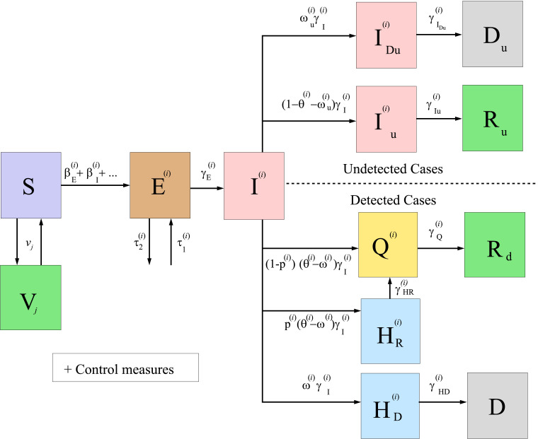
Many models have been proposed to simulate the spread of COVID-19 (see, e.g., [18,52] and the references therein), but, to the best of our knowledge, none of them incorporates the effects of potential SARS-CoV-2 variants together with the vaccines in the spread of COVID-19. In this work, based on the model developed in [29], [30], [31] and improved in [52], we develop a $\theta$-SIR type mathematical model (more precisely, a $\theta -ij$-SVEIHQRD model) able to simulate the possible impact of these types of variants and the vaccines, together with the main mechanisms influencing the disease spread. The new model keeps the compartments and parameters used in [52]. In particular, we use the compartments $S$ (susceptible), $E$ (exposed), $I$ (infectious), $I_{\mathrm{u}}$ (infectious but undetected that will survive the disease), $I_{D_{\mathrm{u}}}$ (infectious but undetected that will die), $Q$ (people in quarantine), $H_R$ (hospitalized that will recover), $H_D$ (hospitalized that will die), $D$ (dead by COVID-19 and detected), $D_{\mathrm{u}}$ (dead by COVID-19 but undetected), $R_{\mathrm{d}}$ (recovered after being previously detected as infectious) and $R_{\mathrm{u}}$ (recovered after being previously infectious but undetected), but we split every infected compartment (i.e., $E,I,I_{\mathrm{u}},I_{D_{\mathrm{u}}},Q,H_R,H_D$) in different subcompartments $E^{\left(i\right)},I^{\left(i\right)},I_{\mathrm{u}}^{\left(i\right)},I_{D_{\mathrm{u}}}^{\left(i\right)},Q^{\left(i\right)},H_R^{\left(i\right)},H_D^{\left(i\right)}$, where $i\in \{1,\cdots ,M\}$ and $M\in \mathbb{N}$ is the number of SARS-CoV-2 variants (including the reference one) that are present in the territory under study.

Furthermore, we incorporate new compartments $V_j$, for people that are immune by vaccination with the $j$-th vaccine, where $j\in \{1,\cdots ,J\}$ and $J\in \mathbb{N}$ is the number of different vaccines being used in the territory under study. We note that people may need to receive several doses and to wait some days (which may depend on the vaccine) to get immunity after vaccination (we point out that it is still not clear if total immunity can be attained with these vaccines, if the vaccinated people may infect others, etc.). For instance, the Comirnaty vaccine needs a second shot 21 days after the first one and wait (in average) 28 days after the first dose to get the maximum efficacy against the virus (see [8], [45]). The Moderna vaccine is also given as two injections, 28 days apart with an efficacy of $94.1\%$ at preventing symptomatic COVID-19, measured starting from 14 days after the second dose (see [15]). We assume that people are in compartment $V_j$ once they get their immunity (not when they get one of the doses). For the sake of simplicity, we assume immunity against all the variants of SARS-CoV-2 for people immune by vaccination or recovered from an infection by any of the variants (other possibilities could be also considered in the model).

The model equations and a diagram summarizing the model (see Fig. 1 ) can be found in Section 2, together with some other details, like formulae for the estimation of the effective reproduction number of each variant of the virus and that of the global disease. The effective reproduction number of each variant must be less than 1 in order to have the spread of the disease under control. The model developed here may be of interest for policy makers, as a tool to evaluate different possible future scenarios.

Fig. 1.

Diagram summarizing the general model for COVID-19 given by system (1)–(2).

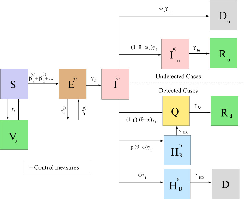
In Section 3, we study the impact in Italy, as a particular example of study case, of the introduction of a new variant of the virus and of the vaccination campaigns. For this, we use a simplified version of the model that is explained in Section 2.

2. General mathematical model

Here, we develop a mathematical model to asses the impact of SARS-CoV-2 variants and vaccination campaigns on the spread of COVID-19 in a considered territory.

In Fig. 1, we show a diagram of the general model developed here, under the assumptions made in Section 1. We remark that, when studying a particular territory, it can be suitable to simplify the general model, according to the data available and the particularities of the case under study. For instance, Fig. 2 below illustrates the diagram of the simplified model used for the particular case of Italy studied in Section 3.

Fig. 2.

Diagram summarizing the simplified model for COVID-19 given by system (9)–(10), applied to the case of Italy.

The evolution of the compartments mentioned above is modeled by the following system of ordinary differential equations:

$$\begin{array}{ccc}\hfill \dot{S}& =& -\frac{S}{N}{\displaystyle \sum _{i=1}^M}({\beta }_E^{\left(i\right)}{E}^{\left(i\right)}+{\beta }_I^{\left(i\right)}{I}^{\left(i\right)}+{\beta }_{I_{\mathrm{u}}}^{\left(i\right)}{I}_{\mathrm{u}}^{\left(i\right)}+{\beta }_{I_{D_{\mathrm{u}}}}^{\left(i\right)}{I}_{D_{\mathrm{u}}}^{\left(i\right)}+{\beta }_{H_R}^{\left(i\right)}{H}_R^{\left(i\right)}+{\beta }_{H_D}^{\left(i\right)}{H}_D^{\left(i\right)})-{\displaystyle \sum _{j=1}^J{v}_j},\hfill \\ \hfill {\dot{E}}^{\left(i\right)}& =& \frac{S}{N}({\beta }_E^{\left(i\right)}{E}^{\left(i\right)}+{\beta }_I^{\left(i\right)}{I}^{\left(i\right)}+{\beta }_{I_{\mathrm{u}}}^{\left(i\right)}{I}_{\mathrm{u}}^{\left(i\right)}+{\beta }_{I_{D_{\mathrm{u}}}}^{\left(i\right)}{I}_{D_{\mathrm{u}}}^{\left(i\right)}+{\beta }_{H_R}^{\left(i\right)}{H}_R^{\left(i\right)}+{\beta }_{H_D}^{\left(i\right)}{H}_D^{\left(i\right)})-{\gamma }_E^{\left(i\right)}{E}^{\left(i\right)}+{\tau }_1^{\left(i\right)}-{\tau }_2^{\left(i\right)},\hfill \\ \hfill {\dot{I}}^{\left(i\right)}& =& {\gamma }_E^{\left(i\right)}{E}^{\left(i\right)}-{\gamma }_I^{\left(i\right)}{I}^{\left(i\right)},\hfill \\ \hfill {\dot{I}}_{\mathrm{u}}^{\left(i\right)}& =& (1-{\theta }^{\left(i\right)}-{\omega }_{\mathrm{u}}^{\left(i\right)}){\gamma }_I^{\left(i\right)}{I}^{\left(i\right)}-{\gamma }_{I_{\mathrm{u}}}^{\left(i\right)}{I}_{\mathrm{u}}^{\left(i\right)},\hfill \\ \hfill {\dot{I}}_{D_{\mathrm{u}}}^{\left(i\right)}& =& {\omega }_{\mathrm{u}}^{\left(i\right)}{\gamma }_I^{\left(i\right)}{I}^{\left(i\right)}-{\gamma }_{I_{D_{\mathrm{u}}}}^{\left(i\right)}{I}_{D_{\mathrm{u}}}^{\left(i\right)},\hfill \\ \hfill {\dot{H}}_R^{\left(i\right)}& =& p^{\left(i\right)}({\theta }^{\left(i\right)}-{\omega }^{\left(i\right)}){\gamma }_I^{\left(i\right)}{I}^{\left(i\right)}-{\gamma }_{H_R}^{\left(i\right)}{H}_R^{\left(i\right)},\hfill \\ \hfill {\dot{H}}_D^{\left(i\right)}& =& {\omega }^{\left(i\right)}{\gamma }_I^{\left(i\right)}{I}^{\left(i\right)}-{\gamma }_{H_D}^{\left(i\right)}{H}_D^{\left(i\right)},\hfill \end{array}$$ (1)

together with

$$\begin{array}{ccc}& & \\ \hfill {\dot{Q}}^{\left(i\right)}& =& (1-p^{\left(i\right)})({\theta }^{\left(i\right)}-{\omega }^{\left(i\right)}){\gamma }_I^{\left(i\right)}{I}^{\left(i\right)}+{\gamma }_{H_R}^{\left(i\right)}{H}_R^{\left(i\right)}-{\gamma }_Q^{\left(i\right)}{Q}^{\left(i\right)},\hfill \\ \hfill \dot{}{R}_{\mathrm{d}}& =& \sum _{i=1}^M{\gamma }_Q^{\left(i\right)}{Q}^{\left(i\right)},\hfill \\ \hfill \dot{}{R}_{\mathrm{u}}& =& \sum _{i=1}^M{\gamma }_{I_{\mathrm{u}}}^{\left(i\right)}{I}_{\mathrm{u}}^{\left(i\right)},\hfill \\ \hfill \dot{}{D}_{\mathrm{u}}& =& \sum _{i=1}^M{\gamma }_{I_{D_{\mathrm{u}}}}^{\left(i\right)}{I}_{D_{\mathrm{u}}}^{\left(i\right)},\hfill \\ \hfill \dot{D}& =& \sum _{i=1}^M{\gamma }_{H_D}^{\left(i\right)}{H}_D^{\left(i\right)},\hfill \\ \hfill \dot{}{V}_j& =& v_j,\hfill \end{array}$$ (2)

for $i\in \{1,\cdots ,M\}$, $j\in \{1,\cdots ,J\}$, where:

• •$M\in \mathbb{N}$ is the number of SARS-CoV-2 variants and $J\in \mathbb{N}$ is the number of vaccines that are being used in the territory under study.
• •
  $v_j\left(t\right)$ is the number of people that get or lose (e.g., because of changes of the vaccine efficacy through time) immunity after getting the $j$-th vaccine (we note that this is different from the number of people vaccinated), per unit time, at time $t$. Here, we have used

  $$v_j\left(t\right)={\int }_0^{t-{\overline{t}}_j}{\dot{e}}_j\left(s\right)u_j(t-s)\mathrm{d}s,$$ (3)

  where $u_j\left(t\right)$ is the number of people that got their first dose of the $j$-th vaccine per unit time, at time $t$, $e_j\left(s\right)$ is the efficacy of the $j$-th vaccine, defined as the ratio of the number of people that is immune by vaccination $s$ days after getting the first dose, and ${\overline{t}}_j$ is the time when the vaccination campaign of the $j$-th vaccine started in the territory under study. We assume that all people receiving the first dose of a vaccine will receive, if they do not get infected, the next necessary doses recommended by the laboratories. More complex formulations can be also used, if necessary. Furthermore, the derivative of $e_j$ (i.e., ${\dot{e}}_j$) can be taken in the distributional sense (see, e.g., [51]), which generalizes the classical notion of derivation and makes it possible to differentiate functions whose derivatives do not exist in the classical sense. In particular, we can use functions $e_j$ which are piecewise constant, as those used in the case of Italy studied below.

  Remark 1

  We point out that, if the vaccination is not only done for people in compartment$S$, then we could use more complex versions of$v_j$. For instance, if we assume that people chosen to get the first dose of a vaccine have not been vaccinated previously and are in compartments$S$,$E^{\left(i\right)}$,$R_{\mathrm{d}}$or$R_{\mathrm{u}}$, then a suitable estimation of$v_j\left(t\right)$, denoted by$v_j^{*}\left(t\right)$, could be

  $$v_j^{*}\left(t\right)={\int }_0^{t-{\overline{t}}_j}{\dot{e}}_j\left(s\right)u_j(t-s)\frac{A_S(t-s)}{F(t-s)}\mathrm{d}s,$$ (4)

  where

  $$F\left(\tau \right)=S\left(\tau \right)+\left(\sum _{i=1}^M\left(E^{\left(i\right)}\left(\tau \right)\right)\right)+R_{\mathrm{d}}(\tau -t_{R_{\mathrm{d}}})+R_{\mathrm{u}}\left(\tau \right)-\sum _{j=1}^J({\int }_{{\overline{t}}_j}^{\tau }{u}_j\left(s\right)\mathrm{d}s-V_j\left(\tau \right))$$

  is an estimation of the number of people that can be chosen to be vaccinated at time$\tau$,$t_{R_{\mathrm{d}}}>0$is the delay (in days) that a person that enters the recovered compartment must wait before being vaccinated,

  $$A_S\left(\tau \right)=S\left(\tau \right)-\sum _{j=1}^J({\int }_{{\overline{t}}_j}^{\tau }\frac{A_S\left(s\right)}{F\left(s\right)}{u}_j\left(s\right)\mathrm{d}s-V_j\left(\tau \right))$$

  is an estimation of the number of people in compartment$S$that can be chosen to be vaccinated at time$\tau$and we take$\frac{A_S\left(\tau \right)}{F\left(\tau \right)}=0$when$F\left(\tau \right)=0$(or$\le 0$in the numerical approximations).4

  We note that the last parentheses in the two previous formulae account for the number of vaccinated people (in the whole population or just in the susceptible compartment, respectively) that have not gotten immunity by vaccination, at time$\tau$. Of course, we can use other possible formulae and also include stratification by age, priority people (like people working in the health system or vulnerable people), event-triggered policies (see, e.g.,[3]), etc. As explained above, in this work, for the sake of simplicity, we just assume that$v_j$is given by(3), since more complex formulae would need the availability of more complete data; the goal here is to get a first idea of possible changes in the behavior of the spread of the pandemic due to new variants of the virus and vaccination campaigns.Note:In the Annex we use(4)(instead of(3)) with updated data obtained at the time of writing a revision of the initial submission of this paper, before publication.

• •
  A detailed description of the other model parameters can be found in [52], taking into account that now the superscript ${}^{\left(i\right)}$ refers to each variant of the virus. For the sake of readability of this work, here we briefly recall their meaning:

  • •
    $N$ is the number of people in the territory before the start of the pandemic.
  • •
    ${\omega }^{\left(i\right)}\left(t\right)\in [0,1]$ is the instantaneous infection detected fatality ratio in the territory, at time $t$; i.e., the proportion of new detected people (after being in compartment $I$) that will die of COVID-19, per unit time, compared to the total number of new infectious people (detected or undetected), per unit time.
  • •
    ${\omega }_{\mathrm{u}}^{\left(i\right)}\left(t\right)\in [0,1]$ is the instantaneous infection undetected fatality ratio in the territory, at time $t$; i.e., the proportion of new undetected people (after being in compartment $I$) that will die of COVID-19, per unit time, compared to the total number of new infectious people (detected or undetected), per unit time.
  • •
    ${\theta }^{\left(i\right)}\left(t\right)\in [{\omega }^{\left(i\right)}\left(t\right),1-{\omega }_{\mathrm{u}}^{\left(i\right)}\left(t\right)]\subset [0,1]$ is the proportion of the number of new infectious people that are detected and documented by the authorities (after being in compartment $I$), per unit time, compared to the total number of new infectious people (detected or undetected), per unit time, at time $t$. If we assume that ${\omega }^{\left(i\right)}=(1+k_{\omega }^{\left(i\right)})\omega$ (for a certain function $\omega$) and, for the sake of simplicity, the proportion of detected cases is the same for all the variants, i.e., ${\theta }^{\left(i\right)}=\theta$ (of course, other possibilities can be also considered) for any $i\in \{1,\cdots ,M\}$, we may compute $\theta \left(t\right)$ as

    $$\begin{array}{c}\hfill \theta \left(t\right)=\{\begin{array}{cc}{\theta }_0,\hfill & \text{if}t\le t_{{\theta }_0},\\ \frac{\omega \left(t\right)}{{\omega }_{\text{CFR}}\left(t\right)}\sum _{i=1}^M(1+k_{\omega }^{\left(i\right)})p_{\mathrm{v}}^{\left(i\right)}\left(t\right),\hfill & \text{if}t>t_{{\theta }_0},\end{array}\end{array}$$ (5)

    where $p_{\mathrm{v}}^{\left(i\right)}\left(t\right)$ is an estimation of the ratio of the infections of variant $i$ over the total number of infections (hence, ${\sum }_{i=1}^M{p}_{\mathrm{v}}^{\left(i\right)}\left(t\right)=1$) and ${\omega }_{\text{CFR}}\left(t\right)$ is a seven-days filtered version of

    $$\frac{d_{\mathrm{r}}(t+s_{H_D}\left(t\right))-d_{\mathrm{r}}(t-r+s_{H_D}(t-r))}{c_{\mathrm{r}}\left(t\right)-c_{\mathrm{r}}(t-r)},$$

    where $c_{\mathrm{r}}\left(t\right)$ is the number of detected cumulative cases at time $t$, $d_{\mathrm{r}}$ is the estimated number of detected cumulative deaths at time $t$, $s_{H_D}\left(t\right)$ is the mean of the duration (days) in compartment $H_D$ of a person that enters that compartment, at time $t$ 5 , and $r$ is the minimum natural number such that $c_{\mathrm{r}}\left(t\right)-c_{\mathrm{r}}(t-r)\ne 0$ and the previous quotient is not greater than 1 (other details can be seen in [52]). Here, we assume that $s_{H_D}$ is a non-decreasing time dependent function (other cases could need a more elaborated estimation).
  • •
    ${\beta }_E^{\left(i\right)},{\beta }_I^{\left(i\right)},{\beta }_{I_{\mathrm{u}}}^{\left(i\right)},{\beta }_{I_{D\mathrm{u}}}^{\left(i\right)},{\beta }_{H_R}^{\left(i\right)},{\beta }_{H_D}^{\left(i\right)}\in [0,\infty )$ are the disease contact rates (day${}^{-1}$) of a person in the respective compartments. We note that some of them may change with time, due to the social distancing control measures. More precisely, we consider that

    $${\beta }_E^{\left(i\right)}\left(t\right)=m\left(t\right){\beta }_{E,0}^{\left(i\right)},{\beta }_I^{\left(i\right)}\left(t\right)=m\left(t\right){\beta }_{I,0}^{\left(i\right)},{\beta }_{I_{\mathrm{u}}}^{\left(i\right)}\left(t\right)=m\left(t\right){\beta }_{I_{\mathrm{u}},0}^{\left(i\right)}\left(\theta \left(t\right)\right),{\beta }_{I_{D_{\mathrm{u}}}}^{\left(i\right)}\left(t\right)=m\left(t\right){\beta }_{I_{D_{\mathrm{u}}},0}^{\left(i\right)}.$$

    Here ${\beta }_{E,0}^{\left(i\right)},{\beta }_{I,0}^{\left(i\right)},{\beta }_{I_{\mathrm{u}},0}^{\left(i\right)}$ and ${\beta }_{I_{D_{\mathrm{u}}},0}^{\left(i\right)}$ are the respective disease contact rates when no control measures are taken. Additionally, $m\in [0,1]$ represents the reduction of those specific disease contact rates, at time $t$, due to the efficiency of the control measures corresponding to social distancing. It is given by (see [29])

    $$m\left(t\right)=\{\begin{array}{cc}(m_0-m_1)\exp (-{\kappa }_1(t-t_0))+m_1,\hfill & \text{if}t\in [t_0,{\lambda }_1],\hfill \\ (m\left({\lambda }_1\right)-m_2)\exp (-{\kappa }_2(t-{\lambda }_1))+m_2,\hfill & \text{if}t\in ({\lambda }_1,{\lambda }_2],\hfill \\ ⋮\hfill & \\ (m\left({\lambda }_{q-1}\right)-m_q)\exp (-{\kappa }_q(t-{\lambda }_{q-1}))+m_q,\hfill & \text{if}t\in ({\lambda }_{q-1},\infty ),\hfill \end{array}$$

    where, for every $i\in \{0,...,q\}$, constants $m_i\in [0,1]$ measure the intensity of the control measures (lower value implies higher intensity), ${\kappa }_i\in [0,+\infty )$ (day${}^{-1}$) simulate the efficiency of the control measures (higher value implies faster effectiveness of the control measures) and ${\lambda }_i\in [t_0,\infty ]$ denote the days of changes of each control strategy.
  • •
    ${\gamma }_I^{\left(i\right)}\left(t\right)\in (0,+\infty )$ is the transition rate (day${}^{-1}$) from compartment $I^{\left(i\right)}$ to compartments $I_{\mathrm{u}}^{\left(i\right)}$, $I_{D_{\mathrm{u}}}^{\left(i\right)}$, $Q^{\left(i\right)}$, $H_R^{\left(i\right)}$ or $H_D^{\left(i\right)}$, at time $t$. Similarly, ${\gamma }_E^{\left(i\right)},{\gamma }_{I_{\mathrm{u}}}^{\left(i\right)}\left(t\right),{\gamma }_{I_{D_{\mathrm{u}}}}^{\left(i\right)}\left(t\right),{\gamma }_Q^{\left(i\right)}\left(t\right),{\gamma }_{H_R}^{\left(i\right)}\left(t\right),$ and ${\gamma }_{H_D}^{\left(i\right)}\left(t\right)\in (0,+\infty )$ denote the transition rates (day${}^{-1}$) from compartments $E^{\left(i\right)}$, $I_{\mathrm{u}}^{\left(i\right)}$, $I_{D_{\mathrm{u}}}^{\left(i\right)}$, $Q^{\left(i\right)}$, $H_R^{\left(i\right)}$ and $H_D^{\left(i\right)}$ to compartments $I^{\left(i\right)}$, $R_{\mathrm{u}}^{\left(i\right)}$, $D_{\mathrm{u}}^{\left(i\right)}$, $R_{\mathrm{d}}^{\left(i\right)}$, $Q^{\left(i\right)}$ and $D^{\left(i\right)}$, respectively, at time $t$.
  • •
    $p^{\left(i\right)}$ is the ratio of the number of new detected infected people that will survive the disease and are hospitalized (they go to compartment $H_R$) over the total number of new detected infected people that will survive the disease (and may also do quarantine, going to compartment $Q^{\left(i\right)}$ without going to hospital).
  • •
    ${\tau }_1^{\left(i\right)}\left(t\right)$ and ${\tau }_2^{\left(i\right)}\left(t\right)$ are the people infected that arrive/leave from/to other territories, per day.

We point out that, due to the emergency of the situation and the lack of data, we have focused on trying to draw general conclusions without aiming to get very precise forecasts. Therefore, for the sake of simplicity, we have not stratified the model by age. This might result in an overestimation of the deaths, because the priority of the vaccines is being given to old people, who have a higher risk of dying from COVID-19.

We note that in system (1)–(2) we have assumed, as stated above, that people in compartment $Q$ are not infectious. In [52], it is explained why this assumption is reasonable for many territories (as, for example, Italy, which is the case studied here) and how to model the general case when this assumption is not suitable.

System (1) is completed with initial non-negative data $S\left(t_0\right)$, $E^{\left(i\right)}\left(t_0\right)$, $I^{\left(i\right)}\left(t_0\right)$, $I_{\mathrm{u}}^{\left(i\right)}\left(t_0\right)$, $I_{D_{\mathrm{u}}}^{\left(i\right)}\left(t_0\right)$, $Q^{\left(i\right)}\left(t_0\right)$, $H_R^{\left(i\right)}\left(t_0\right)$, $H_D^{\left(i\right)}\left(t_0\right)$, $R_{\mathrm{d}}\left(t_0\right)$, $R_{\mathrm{u}}\left(t_0\right)$, $D_{\mathrm{u}}\left(t_0\right)$, $D\left(t_0\right)$ and $V_j\left(t_0\right)$, for all $i\in \{1,\cdots ,M\}$ and $j\in \{1,\cdots ,J\}$.

We note that system (1) is uncoupled with system (2). Therefore, we can solve numerically the whole system (1)–(2) or we can first solve system (1) and then solve each of the equations of (2) as follows:

$$\begin{array}{ccc}\hfill Q^{\left(i\right)}\left(t\right)& =& {\mathrm{e}}^{-{\int }_{t_0}^t{\gamma }_Q^{\left(i\right)}\left(s\right)\mathrm{d}s}(Q^{\left(i\right)}\left(t_0\right)+{\displaystyle {\int }_{t_0}^t{q}^{\left(i\right)}\left(s\right){\mathrm{e}}^{{\int }_{t_0}^s{\gamma }_Q^{\left(i\right)}\left(x\right)\mathrm{d}x}\mathrm{d}s}),\hfill \\ & & \text{with}{q}^{\left(i\right)}=(1-p^{\left(i\right)})({\theta }^{\left(i\right)}-{\omega }^{\left(i\right)}){\gamma }_I^{\left(i\right)}{I}^{\left(i\right)}+{\gamma }_{H_R}^{\left(i\right)}{H}_R^{\left(i\right)},\hfill \\ \hfill R_{\mathrm{d}}\left(t\right)& =& R_{\mathrm{d}}\left(t_0\right)+{\displaystyle \sum _{i=1}^M{\int }_{t_0}^t{\gamma }_Q^{\left(i\right)}\left(s\right)Q^{\left(i\right)}\left(s\right)\mathrm{d}s},\hfill \\ \hfill R_{\mathrm{u}}\left(t\right)& =& R_{\mathrm{u}}\left(t_0\right)+{\displaystyle \sum _{i=1}^M{\int }_{t_0}^t{\gamma }_{I_{\mathrm{u}}}^{\left(i\right)}\left(s\right)I_{\mathrm{u}}^{\left(i\right)}\left(s\right)\mathrm{d}s},\hfill \\ \hfill D_{\mathrm{u}}\left(t\right)& =& D_{\mathrm{u}}\left(t_0\right)+{\displaystyle \sum _{i=1}^M{\int }_{t_0}^t{\gamma }_{I_{D_{\mathrm{u}}}}^{\left(i\right)}\left(s\right)I_{D_{\mathrm{u}}}^{\left(i\right)}\left(s\right)\mathrm{d}s},\hfill \\ \hfill D\left(t\right)& =& D\left(t_0\right)+{\displaystyle \sum _{i=1}^M{\int }_{t_0}^t{\gamma }_{H_D}^{\left(i\right)}\left(s\right)H_D^{\left(i\right)}\left(s\right)\mathrm{d}s,}\hfill \\ \hfill V_j\left(t\right)& =& V_j\left(t_0\right)+{\displaystyle {\int }_{t_0}^t}{v}_j\left(s\right)\mathrm{d}s.\hfill \end{array}$$ (6)

It is important to remark that, if for some territory the model does not include some of the compartments, then these formulae must be changed accordingly.

For the numerical simulations presented in this paper, system (1) was numerically solved, together with the equations of the first line of (2), by applying the classic 4${}^{\text{th}}$ order Runge Kutta method with four stages (RK4) and with four hours as time step (which was tested in [29], [52] and produced suitable stable results). The reason of including the equations of the first line of (2) into the RK4 algorithm was to have the code ready for cases including the possibility of infectiousness of people in compartment $Q$ (as explained above, for the sake of simplicity, we have not considered this case here), which would imply a disease contact rate ${\beta }_Q$ in the equations of the first two lines of (1), coupling in that system the mentioned equations of the first line of (2).

Simultaneously, at each of those time steps, we obtain the solution of system (2) (except for its first equation) given by (6), using the trapezoidal rule for solving the integrals in the formulae. We also note that, in (6), $t_0$ can be changed by any other time $\widehat{t}<t$ (for instance, the numerical time step previous to $t$).

The model is able to generate several outputs of interest, like those described in [52] (taking into account that, here, we introduce the superscript ${}^{\left(i\right)}$, which refers to each variant of the virus). One of those outputs is the effective reproduction number of the $i$-th variant of SARS-CoV-2. It is defined as the number of cases that one infected person of the $i$-th variant of SARS-CoV-2 generates, on average, over the course of its infectious period. Let us see how to compute it.

The model given by equations (1)–(2) assumes that the duration $s_X$ (days) of a person in an infectious compartment $X^{\left(i\right)}\in \{E^{\left(i\right)},I^{\left(i\right)},I_{\mathrm{u}}^{\left(i\right)},I_{D_{\mathrm{u}}}^{\left(i\right)},H_R^{\left(i\right)},H_D^{\left(i\right)}\}$ with constant transition rate ${\gamma }_X^{\left(i\right)}$ (the case of nonconstant transition rates is discussed in Remark 3, to avoid here more complex notation), is an exponentially distributed random variable (see [2]), with probability density function given by $f_X^{\left(i\right)}\left(s_X\right)={\gamma }_X^{\left(i\right)}{\mathrm{e}}^{-{\gamma }_X^{\left(i\right)}{s}_X}$ and mean $\frac{1}{{\gamma }_X^{\left(i\right)}}$. Furthermore, if ${\beta }_X^{\left(i\right)}$ is the disease contact rate of compartment $X^{\left(i\right)}$, then the number of cases generated by an infected person that enters compartment $X^{\left(i\right)}$ at time $z$ and leaves it at time $z+s_X$, while being in that compartment, is

$$r_X^{\left(i\right)}(z,s_X)={\int }_z^{z+s_X}{\beta }_X^{\left(i\right)}\left(\tau \right)\frac{S\left(\tau \right)}{N}\mathrm{d}\tau$$

and, therefore, the expected number of cases generated by an infected person that enters compartment $X^{\left(i\right)}$ at time $z$, while being in that compartment, is

$${\mathcal{R}}_X^{\left(i\right)}\left(z\right)={\int }_0^{\infty }{f}_X^{\left(i\right)}\left(s_X\right)r_X^{\left(i\right)}(z,s_X)\mathrm{d}{s}_X={\int }_0^{\infty }{\gamma }_X^{\left(i\right)}{\mathrm{e}}^{-{\gamma }_X^{\left(i\right)}{s}_X}{\int }_z^{z+s_X}{\beta }_X^{\left(i\right)}\left(\tau \right)\frac{S\left(\tau \right)}{N}\mathrm{d}\tau \mathrm{d}{s}_X.$$

Hence, adding up the contribution of all the infectious compartments related to variant $i$, the model allows to obtain the following estimation of the effective reproduction number of the $i$-th variant of SARS-CoV-2:

$$\begin{array}{ccc}\hfill {\mathcal{R}}_{\mathrm{e}}^{\left(i\right)}\left(t\right)& =& {\int }_0^{\infty }{f}_E^{\left(i\right)}\left(s_E\right)r_E^{\left(i\right)}(t,s_E)\mathrm{d}{s}_E+{\int }_0^{\infty }{\int }_0^{\infty }{f}_E^{\left(i\right)}\left(s_E\right)f_I^{\left(i\right)}\left(s_I\right)r_I^{\left(i\right)}(t+s_E,s_I)\mathrm{d}{s}_E\mathrm{d}{s}_I\hfill \\ & & +{\int }_0^{\infty }{\int }_0^{\infty }{\int }_0^{\infty }(1-{\theta }^{\left(i\right)}(t+s_E+s_I)\hfill \\ & & -{\omega }_u^{\left(i\right)}(t+s_E+s_I))f_E^{\left(i\right)}\left(s_E\right)f_I^{\left(i\right)}\left(s_I\right)f_{I_{\mathrm{u}}}^{\left(i\right)}\left(s_{I_{\mathrm{u}}}\right)r_{I_{\mathrm{u}}}^{\left(i\right)}(t+s_E+s_I,s_{I_{\mathrm{u}}})\mathrm{d}{s}_E\mathrm{d}{s}_I\mathrm{d}{s}_{I_{\mathrm{u}}}+\dots \hfill \\ & =& {\int }_0^{\infty }{\int }_0^{\infty }{\int }_0^{\infty }{\int }_0^{\infty }{\int }_0^{\infty }{\int }_0^{\infty }{\gamma }_E^{\left(i\right)}{\gamma }_I^{\left(i\right)}{\gamma }_{I_{\mathrm{u}}}^{\left(i\right)}{\gamma }_{I_{D_{\mathrm{u}}}}^{\left(i\right)}{\gamma }_{H_R}^{\left(i\right)}{\gamma }_{H_D}^{\left(i\right)}{\mathrm{e}}^{-({\gamma }_E^{\left(i\right)}{s}_E+{\gamma }_I^{\left(i\right)}{s}_I+{\gamma }_{I_{\mathrm{u}}}^{\left(i\right)}{s}_{I_{\mathrm{u}}}+{\gamma }_{H_R}^{\left(i\right)}{s}_{H_R}+{\gamma }_{H_D}^{\left(i\right)}{s}_{H_D})}[r_E^{\left(i\right)}(t,s_E)\hfill \\ & & +r_I^{\left(i\right)}(t+s_E,s_I)+(1-{\theta }^{\left(i\right)}(t+s_E+s_I)-{\omega }_u^{\left(i\right)}(t+s_E+s_I))r_{I_{\mathrm{u}}}^{\left(i\right)}(t+s_E+s_I,s_{I_{\mathrm{u}}})\hfill \\ & & +{\omega }_u^{\left(i\right)}(t+s_E+s_I)r_{I_{D_{\mathrm{u}}}}^{\left(i\right)}(t+s_E+s_I,s_{I_{D_{\mathrm{u}}}})\hfill \\ & & +p^{\left(i\right)}(t+s_E+s_I)({\theta }^{\left(i\right)}(t+s_E+s_I)-{\omega }^{\left(i\right)}(t+s_E+s_I))r_{H_R}^{\left(i\right)}(t+s_E+s_I,s_{H_R})\hfill \\ & & +{\omega }^{\left(i\right)}(t+s_E+s_I)r_{H_D}^{\left(i\right)}(t+s_E+s_I,s_{H_D})]\mathrm{d}{s}_E\mathrm{d}{s}_I\mathrm{d}{s}_{I_{\mathrm{u}}}\mathrm{d}{s}_{I_{D_{\mathrm{u}}}}\mathrm{d}{s}_{H_R}\mathrm{d}{s}_{H_D}.\hfill \end{array}$$

This expression is complex to be applied in numerical simulations, because of the improper integrals. Then, using that $\frac{1}{{\gamma }_X^{\left(i\right)}}$ is the mean of the duration $s_X$ (days) of a person in an infectious compartment $X^{\left(i\right)}$, we may approximate ${\mathcal{R}}_X^{\left(i\right)}\left(z\right)$ by

$${\mathrm{R}}_X^{\left(i\right)}\left(z\right)={\int }_0^{\infty }{f}_X\left(s_X\right)r_X^{\left(i\right)}(z,\frac{1}{{\gamma }_X^{\left(i\right)}})\mathrm{d}{s}_X=r_X^{\left(i\right)}(z,\frac{1}{{\gamma }_X^{\left(i\right)}})={\int }_z^{z+\frac{1}{{\gamma }_X^{\left(i\right)}}}{\beta }_X^{\left(i\right)}\left(\tau \right)\frac{S\left(\tau \right)}{N}\mathrm{d}\tau$$

and, consequently, ${\mathcal{R}}_{\mathrm{e}}^{\left(i\right)}\left(t\right)$ by

$$\begin{array}{ccc}\hfill {\mathrm{R}}_{\mathrm{e}}^{\left(i\right)}\left(t\right)& =& {\int }_0^{\infty }{\int }_0^{\infty }{\int }_0^{\infty }{\int }_0^{\infty }{\int }_0^{\infty }{\int }_0^{\infty }{\gamma }_E^{\left(i\right)}{\gamma }_I^{\left(i\right)}{\gamma }_{I_{\mathrm{u}}}^{\left(i\right)}{\gamma }_{I_{D_{\mathrm{u}}}}^{\left(i\right)}{\gamma }_{H_R}^{\left(i\right)}{\gamma }_{H_D}^{\left(i\right)}{\mathrm{e}}^{-({\gamma }_E^{\left(i\right)}{s}_E+{\gamma }_I^{\left(i\right)}{s}_I+{\gamma }_{I_{\mathrm{u}}}^{\left(i\right)}{s}_{I_{\mathrm{u}}}+{\gamma }_{H_R}^{\left(i\right)}{s}_{H_R}+{\gamma }_{H_D}^{\left(i\right)}{s}_{H_D})}\{r_E^{\left(i\right)}(t,\frac{1}{{\gamma }_E^{\left(i\right)}})\hfill \\ & & +r_I^{\left(i\right)}(t+\frac{1}{{\gamma }_E^{\left(i\right)}},\frac{1}{{\gamma }_I^{\left(i\right)}})+[1-{\theta }^{\left(i\right)}(t+\frac{1}{{\gamma }_E^{\left(i\right)}}+\frac{1}{{\gamma }_I^{\left(i\right)}})-{\omega }_u^{\left(i\right)}(t+\frac{1}{{\gamma }_E^{\left(i\right)}}+\frac{1}{{\gamma }_I^{\left(i\right)}})]r_{I_{\mathrm{u}}}^{\left(i\right)}(t+\frac{1}{{\gamma }_E^{\left(i\right)}}+\frac{1}{{\gamma }_I^{\left(i\right)}},\frac{1}{{\gamma }_{I_{\mathrm{u}}}^{\left(i\right)}})\hfill \\ & & +{\omega }_u^{\left(i\right)}(t+\frac{1}{{\gamma }_E^{\left(i\right)}}+\frac{1}{{\gamma }_I^{\left(i\right)}})r_{I_{D_{\mathrm{u}}}}^{\left(i\right)}(t+\frac{1}{{\gamma }_E^{\left(i\right)}}+\frac{1}{{\gamma }_I^{\left(i\right)}},\frac{1}{{\gamma }_{I_{D_{\mathrm{u}}}}^{\left(i\right)}})\hfill \\ & & +p^{\left(i\right)}(t+\frac{1}{{\gamma }_E^{\left(i\right)}}+\frac{1}{{\gamma }_I^{\left(i\right)}})[{\theta }^{\left(i\right)}(t+\frac{1}{{\gamma }_E^{\left(i\right)}}+\frac{1}{{\gamma }_I^{\left(i\right)}})-{\omega }^{\left(i\right)}(t+\frac{1}{{\gamma }_E^{\left(i\right)}}+\frac{1}{{\gamma }_I^{\left(i\right)}})]r_{H_R}^{\left(i\right)}(t+\frac{1}{{\gamma }_E^{\left(i\right)}}+\frac{1}{{\gamma }_I^{\left(i\right)}},\frac{1}{{\gamma }_{H_R}^{\left(i\right)}})\hfill \\ & & +{\omega }^{\left(i\right)}(t+\frac{1}{{\gamma }_E^{\left(i\right)}}+\frac{1}{{\gamma }_I^{\left(i\right)}})r_{H_D}^{\left(i\right)}(t+\frac{1}{{\gamma }_E^{\left(i\right)}}+\frac{1}{{\gamma }_I^{\left(i\right)}},\frac{1}{{\gamma }_{H_D}^{\left(i\right)}})\}\mathrm{d}{s}_E\mathrm{d}{s}_I\mathrm{d}{s}_{I_{\mathrm{u}}}\mathrm{d}{s}_{I_{D_{\mathrm{u}}}}\mathrm{d}{s}_{H_R}\mathrm{d}{s}_{H_D},\hfill \end{array}$$

which can be rewritten as

$$\begin{array}{ccc}\hfill {\mathrm{R}}_{\mathrm{e}}^{\left(\mathrm{i}\right)}\left(\mathrm{t}\right)& =& {\displaystyle {\int }_t^{t_E^{\left(i\right)}}{\beta }_E^{\left(i\right)}\left(\tau \right)\frac{S\left(\tau \right)}{N}\mathrm{d}\tau +{\int }_{t_E^{\left(i\right)}}^{t_I^{\left(i\right)}}{\beta }_I^{\left(i\right)}\left(\tau \right)\frac{S\left(\tau \right)}{N}\mathrm{d}\tau }\hfill \\ & & {\displaystyle +(1-{\theta }^{\left(i\right)}\left(t_I^{\left(i\right)}\right)-{\omega }_{\mathit{u}}^{\left(\mathit{i}\right)}\left({\mathit{t}}_{\mathit{I}}^{\left(\mathit{i}\right)}\right)){\int }_{t_I^{\left(i\right)}}^{t_{I_{\mathrm{u}}}^{\left(i\right)}}{\beta }_{I_{\mathrm{u}}}^{\left(i\right)}\left(\tau \right)\frac{S\left(\tau \right)}{N}\mathrm{d}\tau +{\omega }_u^{\left(i\right)}\left(t_I^{\left(i\right)}\right){\int }_{t_I^{\left(i\right)}}^{t_{I_{D_{\mathrm{u}}}}^{\left(i\right)}}{\beta }_{I_{D_{\mathrm{u}}}}^{\left(i\right)}\left(\tau \right)\frac{S\left(\tau \right)}{N}\mathrm{d}\tau }\hfill \\ & & {\displaystyle +p^{\left(i\right)}\left(t_I^{\left(i\right)}\right)({\theta }^{\left(i\right)}\left(t_I^{\left(i\right)}\right)-{\omega }^{\left(i\right)}\left(t_I^{\left(i\right)}\right)){\int }_{t_I^{\left(i\right)}}^{t_{H_R}^{\left(i\right)}}{\beta }_{H_R}^{\left(i\right)}\left(\tau \right)\frac{S\left(\tau \right)}{N}\mathrm{d}\tau +{\omega }^{\left(i\right)}\left(t_I^{\left(i\right)}\right){\int }_{t_I^{\left(i\right)}}^{t_{H_D}^{\left(i\right)}}{\beta }_{H_D}^{\left(i\right)}\left(\tau \right)\frac{S\left(\tau \right)}{N}\mathrm{d}\tau ,}\hfill \end{array}$$ (7)

where

$$\begin{array}{c}{t}_E^{\left(i\right)}=t+\frac{1}{{\gamma }_E^{\left(i\right)}},t_I^{\left(i\right)}=t+\frac{1}{{\gamma }_E^{\left(i\right)}}+\frac{1}{{\gamma }_I^{\left(i\right)}},t_{I_{\mathrm{u}}}^{\left(i\right)}=t+\frac{1}{{\gamma }_E^{\left(i\right)}}+\frac{1}{{\gamma }_I^{\left(i\right)}}+\frac{1}{{\gamma }_{I_{\mathrm{u}}}^{\left(i\right)}},t_{I_{D_{\mathrm{u}}}}^{\left(i\right)}=t+\frac{1}{{\gamma }_E^{\left(i\right)}}+\frac{1}{{\gamma }_I^{\left(i\right)}}+\frac{1}{{\gamma }_{I_{D_{\mathrm{u}}}}^{\left(i\right)}}\\ t_{H_R}^{\left(i\right)}=t+\frac{1}{{\gamma }_E^{\left(i\right)}}+\frac{1}{{\gamma }_I^{\left(i\right)}}+\frac{1}{{\gamma }_{H_R}^{\left(i\right)}},t_{H_D}^{\left(i\right)}=t+\frac{1}{{\gamma }_E^{\left(i\right)}}+\frac{1}{{\gamma }_I^{\left(i\right)}}+\frac{1}{{\gamma }_{H_D}^{\left(i\right)}}.\end{array}$$ (8)

Remark 2

Assuming that the fraction of susceptible individuals is constant throughout the calculation of the previous integrals, with

$$\frac{S\left(\tau \right)}{N}=\frac{S\left(t\right)}{N},\text{for}\text{all}\tau \in (t,\max \{t_{I_{\mathrm{u}}}^{\left(i\right)},t_{I_{D_{\mathrm{u}}}}^{\left(i\right)},t_{H_R}^{\left(i\right)},t_{H_D}^{\left(i\right)}\}),$$

and the disease contact rates are constant (which is not realistic for the COVID-19 pandemic, due, for instance, to the changes in time of the control measures), then the effective reproduction number of the $i$-th variant of SARS-CoV-2 can be also estimated as

$$\begin{array}{ccc}\hfill {\overline{\mathrm{R}}}_{\mathrm{e}}^{\left(i\right)}\left(t\right)& =& (\frac{{\beta }_E^{\left(i\right)}}{{\gamma }_E^{\left(i\right)}}+\frac{{\beta }_I^{\left(i\right)}}{{\gamma }_I^{\left(i\right)}}+(1-{\theta }^{\left(i\right)}\left(t_I^{\left(i\right)}\right)-{\omega }_{\mathit{u}}^{\left(\mathit{i}\right)}\left({\mathit{t}}_{\mathit{I}}^{\left(\mathit{i}\right)}\right))\frac{{\beta }_{I_{\mathrm{u}}}^{\left(i\right)}}{{\gamma }_{I_{\mathrm{u}}}^{\left(i\right)}}+{\omega }_u^{\left(i\right)}\left(t_I^{\left(i\right)}\right)\frac{{\beta }_{I_{D_{\mathrm{u}}}}^{\left(i\right)}}{{\gamma }_{I_{D_{\mathrm{u}}}}^{\left(i\right)}}\hfill \\ & & +p^{\left(i\right)}\left(t_I^{\left(i\right)}\right)({\theta }^{\left(i\right)}\left(t_I^{\left(i\right)}\right)-{\omega }^{\left(i\right)}\left(t_I^{\left(i\right)}\right))\frac{{\beta }_{H_R}^{\left(i\right)}}{{\gamma }_{H_R}^{\left(i\right)}}+{\omega }^{\left(i\right)}\left(t_I^{\left(i\right)}\right)\frac{{\beta }_{H_D}^{\left(i\right)}}{{\gamma }_{H_D}^{\left(i\right)}})\frac{S\left(t\right)}{N}.\hfill \end{array}$$

Of course, many other alternatives, for this or other models can be used to estimate the effective reproduction number (see, for instance, [53]).

Remark 3

When the transition rate of an infectious compartment $X\in \{E^{\left(i\right)},I^{\left(i\right)},I_{\mathrm{u}}^{\left(i\right)},I_{D_{\mathrm{u}}}^{\left(i\right)},H_R^{\left(i\right)},H_D^{\left(i\right)}\}$ is given by a time dependent function $\gamma :(0,\infty )\to \mathbb{R}$ such that $\gamma \left(t\right)\ge \underset{\_}{\gamma }>0$, for any value $t\in (0,\infty )$ (for the sake of simplicity of notation, in this remark we avoid in some occasions the use of subscripts and superscripts), the notation and formulae are a little more complicated. If someone enters compartment $X$ at time $z$, the duration $s$ (days) of that person in compartment $X$ is an exponentially distributed random variable, with a probability density function given by

$$f_z\left(s\right)=\gamma (z+s){\mathrm{e}}^{-{\int }_0^s\gamma (z+u)\mathrm{d}u}$$

and mean

$$s\left(z\right)={\int }_0^{\infty }{\mathrm{e}}^{-{\int }_0^s\gamma (z+u)\mathrm{d}u}\mathrm{d}s\le \frac{1}{\underset{\_}{\gamma }}$$

(notice that $s\left(t\right)=\frac{1}{\gamma }$ when $\gamma$ is a constant function). Therefore, the expected number of cases generated by an infected person that enters compartment $X$ at time $z$, while being in that compartment, is

$${\mathcal{R}}_X\left(z\right)={\int }_0^{\infty }{f}_z\left(s\right)r(z,s)\mathrm{d}s={\int }_0^{\infty }\gamma (z+s){\mathrm{e}}^{-{\int }_0^s\gamma (z+u)\mathrm{d}u}{\int }_z^{z+s}{\beta }_X\left(\tau \right)\frac{S\left(\tau \right)}{N}\mathrm{d}\tau \mathrm{d}s.$$

and the model allows to obtain the following estimation of the effective reproduction number of the $i$-th variant of SARS-CoV-2:

$$\begin{array}{ccc}\hfill {\mathcal{R}}_{\mathrm{e}}^{\left(i\right)}\left(t\right)& =& {\int }_0^{\infty }{\int }_0^{\infty }{\int }_0^{\infty }{\int }_0^{\infty }{\int }_0^{\infty }{\int }_0^{\infty }{\gamma }_E^{\left(i\right)}(t+s_E)\cdots {\gamma }_{H_D}^{\left(i\right)}(t+s_E+s_I+s_{H_D}){\mathrm{e}}^{-({\int }_0^{s_E}\gamma (t+u)\mathrm{d}u+\dots +{\int }_0^{s_{H_D}}\gamma (t+s_E+s_I+u)\mathrm{d}u)}\hfill \\ & & [r_E^{\left(i\right)}(t,s_E)+r_I^{\left(i\right)}(t+s_E,s_I)+(1-{\theta }^{\left(i\right)}(t+s_E+s_I)-{\omega }_u^{\left(i\right)}(t+s_E+s_I))r_{I_{\mathrm{u}}}^{\left(i\right)}(t+s_E+s_I,s_{I_{\mathrm{u}}})\hfill \\ & & +{\omega }_u^{\left(i\right)}(t+s_E+s_I)r_{I_{D_{\mathrm{u}}}}^{\left(i\right)}(t+s_E+s_I,s_{I_{D_{\mathrm{u}}}})\hfill \\ & & +p^{\left(i\right)}(t+s_E+s_I)({\theta }^{\left(i\right)}(t+s_E+s_I)-{\omega }^{\left(i\right)}(t+s_E+s_I))r_{H_R}^{\left(i\right)}(t+s_E+s_I,s_{H_R})\hfill \\ & & +{\omega }^{\left(i\right)}(t+s_E+s_I)r_{H_D}^{\left(i\right)}(t+s_E+s_I,s_{H_D})]\mathrm{d}{s}_E\mathrm{d}{s}_I\mathrm{d}{s}_{I_{\mathrm{u}}}\mathrm{d}{s}_{I_{D_{\mathrm{u}}}}\mathrm{d}{s}_{H_R}\mathrm{d}{s}_{H_D}.\hfill \end{array}$$

Now, using that $s_X^{\left(i\right)}\left(z\right)={\int }_0^{\infty }{\mathrm{e}}^{-{\int }_0^s\gamma (z+u)\mathrm{d}u}\mathrm{d}s$ is the mean of the duration $s_X$ (days) of a person in an infectious compartment $X^{\left(i\right)}$, if entering at time $z$ in that compartment, we may approximate ${\mathcal{R}}_X^{\left(i\right)}\left(z\right)$ by

$${\mathrm{R}}_X^{\left(i\right)}\left(z\right)={\int }_0^{\infty }{f}_X\left(s_X\right)r_X^{\left(i\right)}(z,s_X^{\left(i\right)}\left(z\right))\mathrm{d}{s}_X=r_X^{\left(i\right)}(z,s_X^{\left(i\right)}\left(z\right))={\int }_z^{z+s_X^{\left(i\right)}\left(z\right)}{\beta }_X^{\left(i\right)}\left(\tau \right)\frac{S\left(\tau \right)}{N}\mathrm{d}\tau$$

and, consequently, ${\mathcal{R}}_{\mathrm{e}}^{\left(i\right)}\left(t\right)$ by (7), where now

$$\begin{array}{c}{t}_E^{\left(i\right)}=t+s_E^{\left(i\right)}\left(t\right),t_I^{\left(i\right)}=t+s_E^{\left(i\right)}\left(t\right)+s_I^{\left(i\right)}\left(t\right),t_{I_{\mathrm{u}}}^{\left(i\right)}=t+s_E^{\left(i\right)}\left(t\right)+s_I^{\left(i\right)}\left(t\right)+s_{I_{\mathrm{u}}}^{\left(i\right)}\left(t\right),t_{I_{D_{\mathrm{u}}}}^{\left(i\right)}=t+s_E^{\left(i\right)}\left(t\right)+s_I^{\left(i\right)}\left(t\right)+s_{I_{D_{\mathrm{u}}}}^{\left(i\right)}\left(t\right)\\ t_{H_R}^{\left(i\right)}=t+s_E^{\left(i\right)}\left(t\right)+s_I^{\left(i\right)}\left(t\right)+s_{H_R}^{\left(i\right)}\left(t\right),t_{H_D}^{\left(i\right)}=t+s_E^{\left(i\right)}\left(t\right)+s_I^{\left(i\right)}\left(t\right)+s_{H_D}^{\left(i\right)}\left(t\right),\end{array}$$

(which generalizes (8)).

The effective reproduction number of the of SARS-CoV-2 (including all its variants), defined as the expected number of secondary cases produced by one person infected of SARS-CoV-2 (without focusing in a particular variant) at time $t$, can be estimated by

$${\mathrm{R}}_{\mathrm{e}}\left(t\right)=\sum _{i=1}^M\frac{{\mathcal{E}}^{\left(i\right)}\left(t\right)}{{\sum }_{j=1}^M{\mathcal{E}}^{\left(j\right)}\left(t\right)}{\mathrm{R}}_{\mathrm{e}}^{\left(i\right)}\left(t\right),$$

where ${\mathcal{E}}^{\left(i\right)}\left(t\right)=\frac{S}{N}({\beta }_E^{\left(i\right)}{E}^{\left(i\right)}+{\beta }_I^{\left(i\right)}{I}^{\left(i\right)}+{\beta }_{I_{\mathrm{u}}}^{\left(i\right)}{I}_{\mathrm{u}}^{\left(i\right)}+{\beta }_{I_{D_{\mathrm{u}}}}^{\left(i\right)}{I}_{D_{\mathrm{u}}}^{\left(i\right)}+{\beta }_{H_R}^{\left(i\right)}{H}_R^{\left(i\right)}+{\beta }_{H_D}^{\left(i\right)}{H}_D^{\left(i\right)})+{\tau }_1^{\left(i\right)}-{\tau }_2^{\left(i\right)}$ is an estimation of the number of susceptible individuals entering compartment $E^{\left(i\right)}$, per unit time, at time $t$.

Typically, the spread of infection by each variant of SARS-CoV-2 slows down when R${}_{\mathrm{e}}^{\left(i\right)}\left(t\right)<1$. Hence, in order to have the spread of the disease under control, we need that ${\max }_{i\in \{1,\cdots ,M\}}{\text{R}}_{\mathrm{e}}^{\left(i\right)}\left(t\right)<1$. We note that there may be cases with ${\mathrm{R}}_{\mathrm{e}}\left(t\right)<1$ (and, therefore, the number of cases is expected to decrease in the following days) but ${\max }_{i\in \{1,\cdots ,M\}}{\text{R}}_{\mathrm{e}}^{\left(i\right)}\left(t\right)>1$ (and, therefore, there is, at least, one variant of the virus that is spreading, implying that the disease is not under control).

Once the model is built, if we want to use it for a particular country or territory, we need to identify suitable model parameters and functions for the case under study. Some of them can be found in the literature [33]. However, due to the lack of information currently available regarding the behavior of the SARS-CoV-2 and the implicit uncertainty, others need to be estimated. In [52], one can find the details on how to estimate some of the model parameters and particular values of them suitable for the case of Italy.

3. Application to the case of Italy

In order to show the possible impact of the introduction of a new variant of the virus in a territory and the vaccination campaigns, we present here, as an example of application, the results obtained with our model for the case of Italy, one of the countries that has been strongly affected by the pandemic. As explained above, Italy is one of the countries where VOC 202012/01 arrived with one case reported on 20 December 2020 (see [35]), which led the Italian Ministry of Health to forbid flights from the UK to Italy (see [36]).

In Section 3.1, we present a simplified version of our model suitable for the case of Italy. Then, in Section 3.2, we show and discuss the results obtained when we use it to simulate the spread of COVID-19 in this particular country.

3.1. Simplified mathematical model for the case of Italy

The case of the mathematical modeling and simulation of the spread of COVID-19 in Italy was studied in [52], without considering the vaccination campaign which started on 27 December 2020 and taking into account just the reference version (or variant) of SARS-CoV-2.

Here, we study the case of Italy considering vaccination campaigns with the Comirnaty and Moderna vaccines and the introduction in the country of the VOC 202012/01 variant of SARS-CoV-2, which we assume spreads faster than the reference one. For the sake of simplicity, we focus on the case that only the disease contact rates (i.e., the $\beta$s) change in the new variant, with respect to the reference one, keeping the same values used in [52] for all the other parameters (which do not need now the superscript notation ${}^{\left(i\right)}$). The only exceptions are the following: a) we will use the control measures parameters $m_{12}=0.18$ and $m_{13}=0.17$ (which correspond to the intensity of the social distancing strategies started on 23 December 2020 and 7 January 2021, respectively), which is in the range of the multiple values used in [52] in order to study different future scenarios; b) we will use the fatality ratio $\omega =1.4555\%$, which is one of the three options used in [52]. As it is also done in that work, we do not use in this case a compartment for $I_{D_{\mathrm{u}}}$. Of course, many other possibilities can be studied, considering the model above. With these assumptions, and denoting $Q=Q^{\left(1\right)}+Q^{\left(2\right)}$, the simplified model is summarized in Fig. 2 and can now be rewritten, for this case, as the following system of equations:

$$\begin{array}{ccc}\hfill \dot{S}& =& -\frac{S}{N}\sum _{i=1}^2({\beta }_E^{\left(i\right)}{E}^{\left(i\right)}+{\beta }_I^{\left(i\right)}{I}^{\left(i\right)}+{\beta }_{I_{\mathrm{u}}}^{\left(i\right)}{I}_{\mathrm{u}}^{\left(i\right)}+{\beta }_{H_R}^{\left(i\right)}{H}_R^{\left(i\right)}+{\beta }_{H_D}^{\left(i\right)}{H}_D^{\left(i\right)})-\sum _{j=1}^2{v}_j,\hfill \\ \hfill {\dot{E}}^{\left(i\right)}& =& \frac{S}{N}({\beta }_E^{\left(i\right)}{E}^{\left(i\right)}+{\beta }_I^{\left(i\right)}{I}^{\left(i\right)}+{\beta }_{I_{\mathrm{u}}}^{\left(i\right)}{I}_{\mathrm{u}}^{\left(i\right)}+{\beta }_{H_R}^{\left(i\right)}{H}_R^{\left(i\right)}+{\beta }_{H_D}^{\left(i\right)}{H}_D^{\left(i\right)})-{\gamma }_E{E}^{\left(i\right)}+{\tau }_1^{\left(i\right)}-{\tau }_2^{\left(i\right)},\hfill \\ \hfill {\dot{I}}^{\left(i\right)}& =& {\gamma }_E{E}^{\left(i\right)}-{\gamma }_I{I}^{\left(i\right)},\hfill \\ \hfill {\dot{I}}_{\mathrm{u}}^{\left(i\right)}& =& (1-\theta -{\omega }_{\mathrm{u}}){\gamma }_I{I}^{\left(i\right)}-{\gamma }_{I_{\mathrm{u}}}{I}_{\mathrm{u}}^{\left(i\right)},\hfill \\ \hfill {\dot{H}}_R^{\left(i\right)}& =& p(\theta -\omega ){\gamma }_I{I}^{\left(i\right)}-{\gamma }_{H_R}{H}_R^{\left(i\right)},\hfill \\ \hfill {\dot{H}}_D^{\left(i\right)}& =& \omega {\gamma }_I{I}^{\left(i\right)}-{\gamma }_{H_D}{H}_D^{\left(i\right)},\hfill \end{array}$$ (9)

for $i\in \{1,2\}$, together with

$$\begin{array}{ccc}& & \\ \hfill Q\left(t\right)& =& {\mathrm{e}}^{-{\int }_{t_0}^t{\gamma }_Q\left(s\right)\mathrm{d}s}(Q\left(t_0\right)+{\int }_{t_0}^{t}q\left(s\right){\mathrm{e}}^{{\int }_{t_0}^s{\gamma }_Q\left(x\right)\mathrm{d}x}\mathrm{d}s),\hfill \\ & & \text{with}q=\sum _{i=1}^2[(1-p)(\theta -\omega ){\gamma }_I{I}^{\left(i\right)}+{\gamma }_{H_R}{H}_R^{\left(i\right)}]\hfill \\ \hfill R_{\mathrm{d}}\left(t\right)& =& R_{\mathrm{d}}\left(t_0\right)+{\int }_{t_0}^t{\gamma }_Q\left(s\right)Q\left(s\right)\mathrm{d}s,\hfill \\ \hfill R_{\mathrm{u}}\left(t\right)& =& R_{\mathrm{u}}\left(t_0\right)+\sum _{i=1}^2{\int }_{t_0}^t{\gamma }_{I_{\mathrm{u}}}\left(s\right)I_{\mathrm{u}}^{\left(i\right)}\left(s\right)\mathrm{d}s,\hfill \\ \hfill D_{\mathrm{u}}\left(t\right)& =& D_{\mathrm{u}}\left(t_0\right)+\sum _{i=1}^2{\int }_{t_0}^t{\omega }_{\mathrm{u}}\left(s\right){\gamma }_I\left(s\right)I^{\left(i\right)}\left(s\right)\mathrm{d}s,\hfill \\ \hfill D\left(t\right)& =& D\left(t_0\right)+\sum _{i=1}^2{\int }_{t_0}^t{\gamma }_{H_D}\left(s\right)H_D^{\left(i\right)}\left(s\right)\mathrm{d}s,\hfill \\ \hfill V_j\left(t\right)& =& V_j\left(t_0\right)+{\int }_{t_0}^t{v}_j\left(s\right)\mathrm{d}s.\hfill \end{array}$$ (10)

for $j\in \{1,2\}$.

We will assign the index $i=1$ to the reference SARS-CoV-2 virus, the index $i=2$ to the new variant VOC 202012/01, the index $j=1$ to the Comirnaty vaccine and the index $j=2$ to the Moderna vaccine. For the reference virus, we use the values of the parameters given in [52]. To model that the new variant spreads faster than the reference one, we assume that ${\beta }_X^{\left(2\right)}=(1+k){\beta }_X^{\left(1\right)}$, with $k>0$, for all $X\in \{E,I,I_{\mathrm{u}},I_{D_{\mathrm{u}}},H_R,H_D\}$. In other words, the disease contact rates of the variant are $100\times k$% higher than the disease contact rates of the reference version of the virus.

The initial data considered to run the simulations are detailed in [52] for the reference variant. According to [12], the first reported cases of the new variant in Italy were imported from the UK to different Italian regions. Here, we enumerate them by date of confirmation: 20 December 2020, one case in Lazio; 21-22 December 2020, two cases in Apulia; 23-24 December 2020, two cases in Lombardy; 24 December 2020, three cases in Veneto; 26 December 2020, six cases in Naples. Those detected cases were introduced into system (9) using parameter ${\tau }_1^{\left(2\right)}$. For the sake of simplicity, we assume that they arrived in exposed state $E$ and we introduce them twelve days before its official date of confirmation (taking into account one day of delay in the notification and eleven days that they spend in average in states $E$ and $I$ before its detection). All the time series used in this work, including the one with the imported cases, are available at https://github.com/momat-ucm/T-SIR-T.

We use equation (3) for both vaccines with the following efficacy functions:

• •
  For the Comirnaty vaccine, we take

  $$e_1\left(s\right)=\{\begin{array}{cc}0,\hfill & \text{if}0\le s<12\text{days},\hfill \\ 0.524,\hfill & \text{if}12\text{days}\le s<21\text{days},\hfill \\ 0.905,\hfill & \text{if}21\text{days}\le s<28\text{days},\hfill \\ 0.948,\hfill & \text{if}28\text{days}\le s,\hfill \end{array}$$ (11)

  which corresponds to the Comirnaty vaccine efficacy. These values, given in [49], must be taken with caution, since, as said in that work, their “study was not designed to assess the efficacy of a single-dose regimen”.
  Then, the $e_1$ derivative in the distributional sense is

  $${\dot{e}}_1\left(s\right)=0.524\delta (s-12)+(0.905-0.524)\delta (s-21)+(0.948-0.905)\delta (s-28),$$

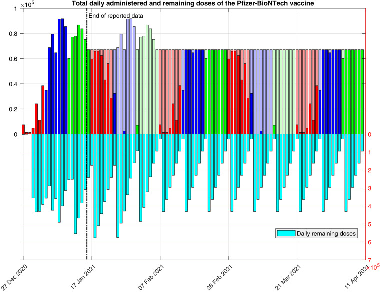
  where $\delta (·)$ is the Delta Dirac function, and (3) may be rewritten in this case as

  $$v_1\left(t\right)=0.524u_1(t-12)+(0.905-0.524)u_1(t-21)+(0.948-0.905)u_1(t-28).$$
  The Comirnaty vaccine was the first vaccine used in this country, with a first batch of 9,750 doses received on 26 December 2020 (see [38]). The vaccination campaign continued the following days with a rate of around 470,000 doses per week (see [39]). The data of the vaccines already administered (at the time of writing) that we use here for our simulations were taken on 17 January 2021 from the Italian official repository [9]. For the sake of simplicity, we do not consider here the possibility of using an additional dose from the vials that were supposed to contain five doses of the Pfizer-BioNtech vaccine. Taking into account this information and assuming that the second dose of the Comirnat vaccine will be administered 21 days after the first one, we use the function $u_1$ defined as follows:

  $$u_1\left(t\right)=\{\begin{array}{cc}\text{Official}\text{reported}\text{values},\hfill & \text{if}t<\text{16}\text{January}\text{2021}\hfill \\ 470,000/7,\hfill & \text{if}\text{16}\text{January}\text{2021}\le t<\text{17}\text{January}\text{2021},\hfill \\ \max (470,000/7-u_1(t-21),0),\hfill & \text{if}t\ge \text{17}\text{January}\text{2021}.\hfill \end{array}$$ (12)

  In Fig. 3 , we show the total daily amount of remaining and (first and second) administered doses, resulting from the use of this function. We note that, with this choice, from the seventh week, every day there will be a constant number of 470,000/7 vaccines administered per day (first plus second doses) and function $u_1$ is periodic, with period of 6 weeks, from the fourth week. Of course, other choices of function $u_1$ (for instance if it is assumed that fewer doses are administered on weekends, etc.) can be also used.
• •
  For the Moderna vaccine, we consider

  $$e_2\left(s\right)=\{\begin{array}{cc}0,\hfill & \text{if}0\le s<7\text{days},\hfill \\ 0.545,\hfill & \text{if}7\text{days}\le s<14\text{days},\hfill \\ 0.943,\hfill & \text{if}14\text{days}\le s<28\text{days},\hfill \\ 1,\hfill & \text{if}28\text{days}\le s<42\text{days},\hfill \\ 0.941,\hfill & \text{if}42\text{days}\le s,\hfill \end{array}$$ (13)

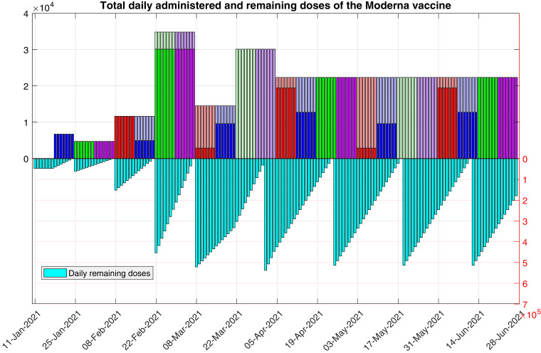
  which corresponds to values for the Moderna vaccine efficacy deduced from [1]. Again, these values must be taken with caution, since this study was not designed to assess the efficacy function along different time intervals and few data are included.
  Then, the $e_2$ derivative in the distributional sense is

  $${\dot{e}}_2\left(s\right)=0.545\delta (s-7)+(0.943-0.545)\delta (s-14)+(1-0.943)\delta (s-28)-(1-0.941)\delta (s-42),$$

  and (3) may be rewritten in this case as

  $$v_2\left(t\right)=0.545u_2(t-7)+(0.943-0.545)u_2(t-14)+(1-0.943)u_2(t-28)-(1-0.941)u_2(t-42).$$
  Regarding the Moderna vaccine, according to different media, such as [19], [54], the first 47,000 doses arrived in Italy between 11 and 12 January 2021, and their administration was programmed to start one week later, on 18 January 2021. Then, the government plans to increase the amount of dispatched doses every two weeks, reaching a total of 764,000 doses on 22 February 2021. Furthermore, according to [24], 536,000 more doses would arrive during March, adding up a total of 1.3 million doses of the Moderna vaccine. Taking into account this information and assuming that the second dose of the Moderna vaccine will be administered 28 days after the first one, we use the function $u_2$ defined as follows:

  $$u_2\left(t\right)=\{\begin{array}{cc}47,000/7,\hfill & \text{if}\text{18}\text{January}\text{2021}\le t<\text{25}\text{January}\text{2021},\hfill \\ 66,000/14,\hfill & \text{if}\text{25}\text{January}\text{2021}\le t<\text{8}\text{February}\text{2021},\hfill \\ 163,000/14,\hfill & \text{if}\text{8}\text{February}\text{2021}\le t<\text{15}\text{February}\text{2021},\hfill \\ 163,000/14-u_2(t-28),\hfill & \text{if}\text{15}\text{February}\text{2021}\le t<\text{22}\text{February}\text{2021},\hfill \\ 488,000/14-u_2(t-28),\hfill & \text{if}\text{22}\text{February}\text{2021}\le t<\text{8}\text{March}\text{2021},\hfill \\ 536,000/12-u_2(t-14)-u_2(t-28),\hfill & \text{if}\text{8}\text{March}\text{2021}\le t<\text{22}\text{March}\text{2021},\hfill \\ 0,\hfill & \text{if}\text{22}\text{March}\text{2021}\le t<\text{5}\text{April}\text{2021},\hfill \\ 536,000/24-u_2(t-28),\hfill & \text{if}\text{5}\text{April}\text{2021}\le t.\hfill \end{array}$$ (14)

  In the previous function we assume that, ideally, on the first four weeks all the available doses are administered, and in the following ones, priority is given to second shots. We note that this implies to keep some vaccines in deposit in the week from 8 to 21 March 2021, for future second doses in the week from 22 March 2021 to 4 April 2021.

  In Fig. 4 , we show the total daily amount of remaining and (first and second) administered doses, resulting from the use of this function. We note that, with this choice, from the twelfth week, every day there will be a constant number of 536,000/24 vaccines administered per day (first plus second doses), and function $u_2$ is periodic, with period of 8 weeks, from the eighth week. Again, other choices of function $u_2$ are also possible.

Fig. 3.

Total daily amount of remaining and administered doses of the Comirnaty vaccine, as determined by function $u_1$. The darker colors correspond to first doses (i.e., the values of $u_1$), and the lighter colors correspond to second doses. The last plateau corresponds to $470,000/7$ doses.

Fig. 4.

Total daily amount of remaining and administered doses of the Moderna vaccine, as determined by function $u_2$. The darker colors correspond to first doses (i.e., the values of $u_2$), and the lighter colors correspond to second doses. The last plateau corresponds to $536,000/24$ doses.

3.2. Results for the case of Italy

For the results presented in the section, we used the simplified model, parameters and data described in Section 3.1. Following the conclusions of the 18 December report of the UK’s New and Emerging Respiratory Virus Threats Advisory Group (mentioned above) regarding the transmissibility of VOC-202012/01, we considered in the model an increase of 39% and 93% of the variant’s disease contact rates (the $\beta$s), with respect to the reference’s ones, since the R${}_{\mathrm{e}}$ value (i.e., the effective reproduction number) is proportional to these parameters. We point out that the other possible increases mentioned above are between those two values. We only report here the results corresponding to the increase of 93%, since the simulations done with an increase of 39% are quite similar to those obtained without considering a second variant, for the time intervals studied here.

We have simulated two different scenarios involving the new variant and vaccines: a) the control measures active in Italy as of 17 January 2021 (at the time of writing) are maintained over time (see Section 3.2.1), b) the control measures active in Italy as of 17 January are relaxed on 1 March 2021 (see Section 3.2.2).

In Section 3.2.3, we analyze and discuss the obtained results.

3.2.1. The control measures active in Italy as of 17 January 2021 are maintained over time.

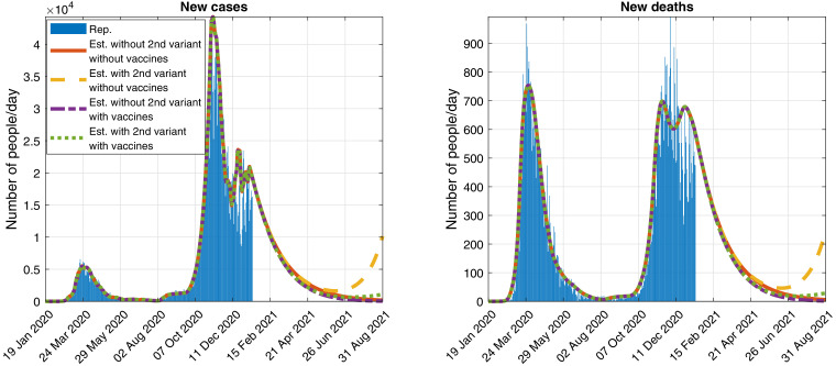
In Fig. 5 , we show a possible evolution of the number of daily detected cases and deaths, with and without vaccination campaigns and new variant, when keeping the control measures used at the time of writing.

Fig. 5.

Official reported (Rep.) data and simulation (Est.) of the evolution of the daily detected (Left) cases and (Right) deaths, assuming that the control measures as of 17 January 2021 are maintained and considering the reference virus and a second variant of SARS-CoV-2 that spreads a 93% faster.

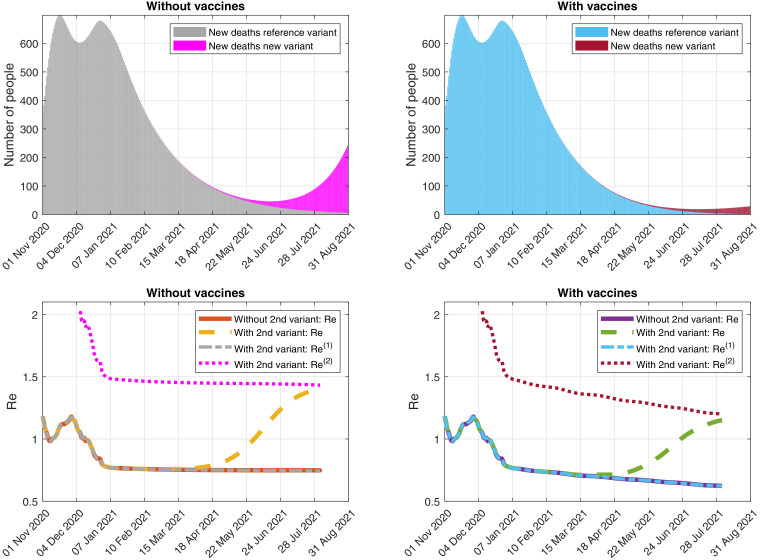
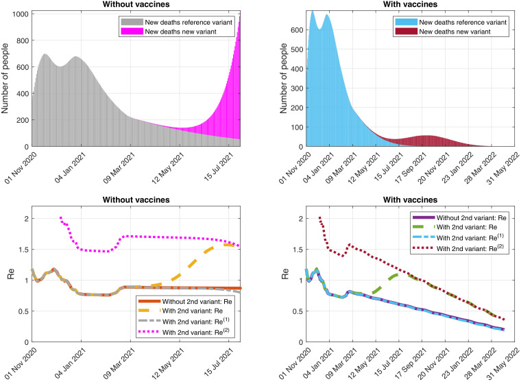
In Fig. 6 -(Top), we can see the simulation of the evolution of the daily detected deaths caused by each variant, with and without vaccination campaigns. In Fig. 6-(Bottom), we illustrate the possible evolution of the effective reproduction numbers with and without vaccination campaigns and new variant.

Fig. 6.

Simulation of the evolution of (Top) the daily detected deaths caused by each variant and (Bottom) the effective reproduction numbers, assuming that the control measures as of 17 January 2021 are maintained and considering the reference virus and a second variant of SARS-CoV-2 that spreads a 93% faster. (Right) With and (Left) without vaccines.

3.2.2. The control measures active in Italy as of 17 January 2021 are relaxed on 1 March 2021.

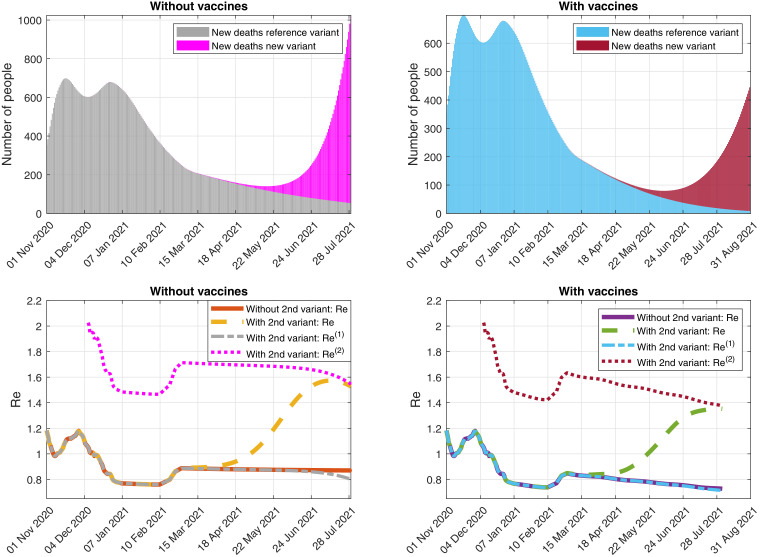
In Figs. 7 and 8, we show some results of the simulations, if we assume that the control measures are relaxed on 1 March 2021, with $m_{14}=0.20$. It is a value similar to the one we estimated in [52] for the period between 13 November and 23 December 2020 (before Christmas).

Fig. 7.

Official reported data and simulation of the evolution of the daily detected (Left) cases and (Right) deaths, assuming that the control measures are relaxed on 1 March 2021 (with $m_{14}=0.20$) and considering a second variant of SARS-CoV-2 that spreads a 93% faster.

Fig. 8.

Simulation of the evolution of (Top) the daily detected deaths caused by each variant and (Bottom) the effective reproduction numbers, assuming that the control measures are relaxed on 1 March 2021 (with $m_{14}=0.20$) and considering a second variant of SARS-CoV-2 that spreads a 93% faster. (Right) With and (Left) without vaccines.

Finally, in Figs. 9 and 10, we show some results of the simulations, if we also assume that the rate of vaccination is twice the one defined by $u_1$ and $u_2$ (see 12 and 14), from 18 January 2021.

Fig. 9.

Official reported data and simulation of the evolution of the daily detected (Left) cases and (Right) deaths, assuming that the control measures are relaxed on 1 March 2021 (with $m_{14}=0.20$) and the rate of vaccination is twice the one defined by $u_1$ and $u_2$ (see 12 and 14), from 18 January 2021, and considering a second variant of SARS-CoV-2 that spreads a 93% faster.

Fig. 10.

Simulation of the evolution of (Top) the daily detected deaths caused by each variant and (Bottom) the effective reproduction numbers, assuming that the control measures are relaxed on 1 March 2021 (with $m_{14}=0.20$) and the rate of vaccination is twice the one defined by $u_1$ and $u_2$ (see 12 and 14), from 18 January 2021, and considering a second variant of SARS-CoV-2 that spreads a 93% faster. (Right) With and (Left) without vaccines.

3.2.3. Discussion

From the figures above, we observe that, for the scenarios without the introduction of the new variant, the pandemic is under control if we keep the control measures as of 17 January 2021 and also if the control measures are slightly relaxed on 1 March 2021. In those cases, the effective reproduction numbers are below 1 and the daily numbers of new cases and deaths are constantly decreasing since January 2021.

On the opposite, when introducing the second variant of the virus, the behaviour of the pandemic depends on the use or not of vaccines. Indeed, without the administration of vaccines, the number of cases and deaths would start increasing in June and the situation would become out of control. Actually, in that context, the problem would have started before that, with the introduction of the second variant, which had an associated effective reproduction number (${\mathrm{R}}_{\mathrm{e}}^{\left(2\right)}$) greater than 1. Therefore, even if in January the global effective reproduction number (${\mathrm{R}}_{\mathrm{e}}$) is less than 1 and the number of total cases and deaths is decreasing, the number of cases and deaths associated to the second variant would increase leading the pandemic to a next wave. In other words, in contrast with common thoughts, ${\mathrm{R}}_{\mathrm{e}}<1$ is not enough for having the spread of the disease under control, if a more contagious new variant is active.

The administration of the vaccine should help to avoid this dramatic situation. In that case, although ${\mathrm{R}}_{\mathrm{e}}^{\left(2\right)}>1$, its values are lower than in the previous scenario (i.e., without vaccine) and it exhibits a continuous decreasing trend. Thus, the numbers of daily new cases and deaths are considerably reduced in comparison with the previous case. However, although not represented here, eventually there could be a smaller new wave that would finish once ${\mathrm{R}}_{\mathrm{e}}^{\left(2\right)}<1$.

Furthermore, maintaining the control measures to their current level seems to be necessary to keep the situation under control, if we keep the expected (at the time of writing) rate of vaccination. Actually, as can be seen in Figs. 7 and 8, relaxing those control measures in the near future could produce a huge increase in the pandemic magnitude, with or without vaccines. In order to be able to relax these control measures (which might have a terrible economic impact if they are maintained for a long time), it would be necessary to increase significantly the rate of vaccination. For instance, we show in Figs. 9 and 10, the simulations obtained when we relax the control measures (as before) but the rate of vaccination is doubled from 18 January 2021. It is clear that, in this scenario, the pandemic would be under control.

From all those results, we conclude that, although the situation in Italy seems to be actually under control, variant VOC 202012/01 (whose associated effective reproduction number could be greater than 1) might produce situations with an uncontrolled new wave even with the current rate of vaccination and control measures. Keeping the control measures and increasing the rate of vaccination seem necessary.

4. Conclusion

We have developed a mathematical model that is able to simulate the impact of SARS-CoV-2 variants and vaccines on the spread of COVID-19. It is based on the models proposed in [29], [52], which were able to simulate other main mechanisms influencing the disease spread. For the sake of simplicity, we have not included in the model stratification by age, stochasticity and other features that are relevant in this context. The reason is that the goal here is to get a first idea (as soon as possible, because of the emergency of the situation) of possible changes in the behavior of the spread of the pandemic due to new variants of the virus and vaccination campaigns. Furthermore, a more complex model would need the availability of more complete data.

The model is ready (and freely available) to be used with real data in any territory where sufficient information about the disease is gathered by the authorities.

We have applied the model to the particular case of Italy, which has allowed to draw some conclusions. The results show that the current rates of vaccination in that country might not be enough, for example if the control measures are relaxed, to avoid a next wave of the disease. Actually, a potentially more contagious new variant (like the so-called British Variant: VOC 202012/01) may lead the disease to a new wave unless the vaccination rate is increased or very strict control measures are maintained for a long time.

We also obtain formulae for the effective reproduction number (${\mathrm{R}}_{\mathrm{e}}^{\left(i\right)}$) of each variant ($i$) and also for the effective reproduction number (${\mathrm{R}}_{\mathrm{e}}$) of the whole disease. Interestingly, we show that, in contrast with common thoughts, ${\mathrm{R}}_{\mathrm{e}}<1$ is not enough for having the spread of the disease under control, if a more contagious variant $i$, with ${\mathrm{R}}_{\mathrm{e}}^{\left(i\right)}>1$, is active.

Note: The results presented previously were obtained with official data reported up to 17 January 2021 and submitted to the journal on 22 January 2022. In this final version of the article (submitted to the journal on 26 May 2021), following a reviewer’s suggestion we have added in the Annex an update of the situation with official data reported up to 25 May 2021. This update confirms what was said in the conclusions:

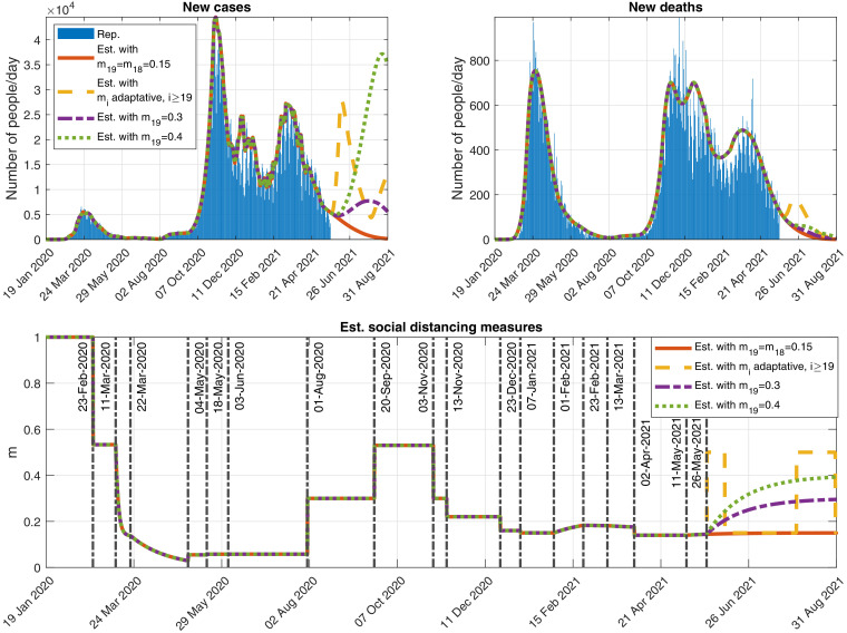
• •A new variant has lead the disease to a new wave (the third one) in Italy (see Fig. 14).
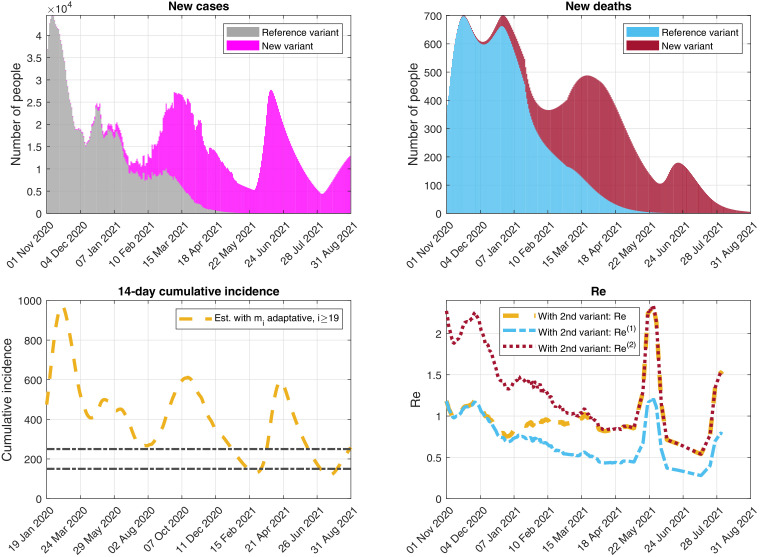
• •Although ${\mathrm{R}}_{\mathrm{e}}<1$ when submitting the first version of this article, the pandemic was not under control, with ${\mathrm{R}}_{\mathrm{e}}^{\left(2\right)}>1$ and eventually ${\mathrm{R}}_{\mathrm{e}}$ getting bigger than 1 (see Fig. 15).

Fig. 14.

Outputs obtained when simulating possible future scenarios described in the Annex. Top-left: New detected cases per day. Top-right: New detected deaths per day. Bottom: Function modeling the social distancing measures.

Fig. 15.

Outputs obtained when simulating the future scenario with adaptative control measures (yellow scenario) described in the Annex. Top-left: Daily detected cases caused by each variant. Top-right: Daily detected deaths caused by each variant. Bottom-left: 14-day cumulative incidence. Bottom-right: Effective reproduction numbers.

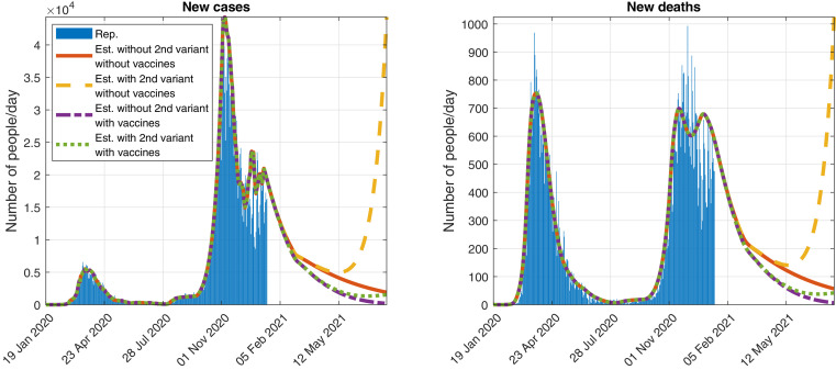
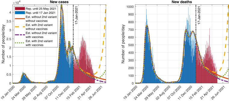
We point out that the simulations of the scenarios studied in Section 3.2 (which correspond to the initial submission of this article) fit quite well the official data reported by the Italian authorities for one month approximately concerning new cases and even for a longer period of time regarding new deaths (see Fig. 11 ). After that month, there are differences in the dates and magnitudes of the third wave, due to several reasons (see the Annex): poor data available in the literature (when the first version of this article was submitted) about people in Italy infected with the new variant, the Italian authorities relaxed the control measures earlier than the date considered in the scenarios, more information appeared later in the literature showing a higher new variant mortality rate for the new variant, the official data/estimations regarding the vaccination campaign have changed, difficulty of the SIR type models to estimate the evolution of an epidemic/pandemic for long periods of time (due to the sensitivity of its equations to some of their parameters), etc.

Fig. 11.

Official data reported up to 25 May 2021, compared to the simulations of the scenarios described in Section 3.2, which appeared in the initial version of this article (see Fig. 7), submitted to the journal on 22 January 2022 using official data reported up to 17 January 2021. Evolution of the daily detected (Left) cases and (Right) deaths, assuming several scenarios described in Section 3.2.

Code and data availability

The codes and data used in this paper are freely available at https://github.com/momat-ucm/T-SIR-T and at https://www.ucm.es/momat/software-momat. The core model was written in Java. The figures were generated with MATLAB.

CRediT author statement

All authors contributed equally to the work.

Declaration of Competing Interest

The authors declare that they have no known competing financial interests or personal relationships that could have appeared to influence the work reported in this paper.

Appendix

In the version of this article initially submitted on 22 January 2021 to Communications in Nonlinear Science and Numerical Simulation, the case of Italy studied in Section 3.2 was written using official data reported up to 17 January 2021 to validate the model and analyze several future scenarios. Here, in Fig. 11, we compare some of the future scenarios described in that initial version, in particular those included in Fig. 7, with the official data reported up to 25 May 2021. In the current version, written later as a revised version of the submitted paper, we have kept everything that was computed/estimated using those data (including the values of the parameters and the figures with the outcomes of the simulations). Furthermore, following a reviewer’s suggestion, in this Annex we show an update of the situation in Italy, using official data reported up to 25 May 2021. It is important to remark that, in all the simulations shown in this Annex, we keep the same parameter values as those given in the version of the paper initially submitted to the journal (with official data reported up to 17 January 2021, as mentioned above), with the following updates based on new data:

• 1.Update of$\tau$: In Section 3.1, we assumed that the first cases of the new variant in Italy arrived on their dates of confirmation, which were between 20 and 26 December 2020. However, according to recent publications (see [20] and [22]), the first reported 13 cases were imported from the UK to Italy around 7 December 2020, i.e., two weeks before our previously considered date. Therefore, in this Annex, we have advanced their introduction into system (9) through parameter ${\tau }_1^{\left(2\right)}$ fourteen days with respect to the scenarios studied in Section 3.2. Furthermore, there exist suspicions that this new variant arrived to Italy before those dates (see, e.g., [34] or [55]). Thus, we consider two additional first cases on 8 October 2020, which means ${\tau }_1^{\left(2\right)}($8 October 2020$)=2$. These values have been obtained by calibration, taking into account the percentages of the new variant officially reported by the Italian authorities in [28] and detailed below.
• 2.
  Update of the control measures: In the scenarios studied in Section 3.2, we considered (just as a hypothetical situation) a relaxation of the control measures on 1 March 2021. Nevertheless, the Italian authorities relaxed the measures on 1 February 2021 (see [41]) which generated, from a strictly quantitative point of view, differences between the scenarios and the observations. We have also changed the control measures on 23 December and 7 January after a calibration using more data than those available when submitting the first version of this paper. In Table 1, we include the parameters used to model the control measures from 23 December 2020. The parameters considered before this date are detailed in our previous work [52]. The dates of application of the different control measures in Table 1 have been consulted in the following references [21], [41] and [44], and the efficiency and intensity values have been calibrated using the official data available in [46].

  Table 1.

  Summary of the parameters used to model the control measures corresponding to the days after 23 December 2020. Time intervals with different measures are indexed with $i\in \{12,13,14,15,16,17,18,19\}$.

  Date of application	Efficiency	Intensity	Type
  (${\lambda }_{i-1}$)	(${\kappa }_i$)	($m_i$)
  23 December 2020	62.0015	0.16	Restriction
  7 January 2021	62.0015	0.15	Restriction
  1 February 2021	0.0362	0.21	Relaxation
  23 February 2021	0.0362	0.18	Restriction
  13 March 2021	0.0362	0.17	Restriction
  2 April 2021	62.0015	0.14	Restriction
  11 May 2021	0.0362	0.15	Relaxation
  26 May 2021	Different	Different	Different
  	scenarios	scenarios	scenarios

• 3.Update of$\omega$: New information (not available when we submitted the first version of this article) indicates (see [23]) a 58% higher mortality rate of the VOC 202012/01 variant. Therefore, we consider now two different functions ${\omega }^{\left(1\right)}$ and ${\omega }^{\left(2\right)}=(1+k_{\omega }){\omega }^{\left(1\right)}$, where $k_{\omega }=0.58$.

  Furthermore, one of the major benefits of the vaccination campaign is the reduction of the disease death rate (see, e.g., [50]). For the sake of simplicity, here, we assume that vaccinated people will not die due to COVID-19. Furthermore, regarding the current vaccination strategy in Italy, vulnerable people are vaccinated in priority (currently, one of the main criteria is the age of a person, despite the fact that other factors are also taken into account such as the professions at risk, see [37]). It has been observed that older people present higher death rates than younger ones (see, e.g., [32]). Thus, the vaccination campaign implies a decrease in the overall disease death rate.

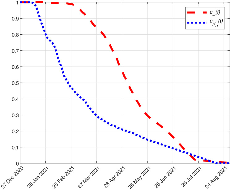
  To model this effect, we have considered a suitable decreasing function $c_{\omega }\left(t\right)\in [0,1]$ that multiplies the value of ${\omega }^{\left(1\right)}$ previous to the Italian vaccination campaign (i.e., ${\omega }^{\left(1\right)}=1.4555\%$, as stated in Section 3.1). More precisely, we use ${\omega }^{\left(1\right)}\left(t\right)=1.4555c_{\omega }\left(t\right)$, with

  $$c_{\omega }\left(t\right)=\frac{\tilde{\omega }\left(t\right)}{\tilde{\omega }\left(t_{\text{vac}}\right)},\text{if}t>t_{\text{vac}}\text{,}\text{and}\text{1}\text{elsewhere,}$$

  where $t_{\text{vac}}=$27 December 2020 is the initial time of the vaccination campaign and $\tilde{\omega }\left(t\right)$ is an estimation of the Case Fatality Ratio (CFR) at time $t$ taking into account the number and age of people that have been vaccinated. In particular, $\tilde{\omega }\left(t\right)$ is given by

  $$\tilde{\omega }\left(t\right)=\sum _{i=1}^{N_{\text{age}}}\frac{N_i(t-t_{\text{vd}})}{{\sum }_i^{N_{\text{age}}}{N}_i(t-t_{\text{vd}})}{\omega }_{\text{CFR},i},$$

  where $N_{\text{age}}\in \mathbb{N}$ is the number of groups used to classify the population by its age (here, intervals of 10 years, [37]) and ordered from younger (i.e., $i=1$) to older (i.e., $i=N_{\text{age}}$) people, $N_i\left(t\right)$ is the number of non-vaccinated people with an age included in group $i$ at time $t$, ${\omega }_{\text{CFR},i}$ is the CFR of people with an age in interval $i$ reported on 16 December 2020 in [25] (which is the latest report available before the beginning of the vaccination campaign) and $t_{\text{vd}}\in \mathbb{N}$ is the delay (in days) between the injection of the first dose of vaccine and the protection from death.

  To estimate $t_{\text{vd}}$, we have considered the official Italian situation reports (see [25]), and estimated that between 16 December 2021 and 14 April 2021, the CFR decreased by 28.63%. For the sake of simplicity, we assume that this decrease is mainly due to the effect of the vaccination campaign. Thus, in order to fit this value (i.e., $c_{\omega }($14 April 2021$)\approx 71.37\%$), we set $t_{\text{vd}}=12$ days and obtain that $c_{\omega }($14 April 2021$)=71.32\%$.

  Finally, in order to estimate the evolution of $N_i\left(t\right)$ up to the end of the considered simulation, if $t_{\text{data}}$ is the latest date of available data, for t > t _data we use the estimation given by

  $$N_i\left(t\right)=\text{max}(N_i\left(t_{\text{data}}\right)-(t-t_{\text{data}})\times \widetilde{N_i}+\sum _{j=i}^{N_{\text{age}}}\left(\text{min}(N_j\left(t_{\text{data}}\right)-(t-t_{\text{data}})\times \widetilde{N_j},0)\right),0),$$

  where $\widetilde{N_i}=\frac{1}{7}{\sum }_{j=t_{\text{data}}-6}^{t_{\text{data}}}{N}_t\left(j\right)-N_t(j-1)$ is the average daily number of people vaccinated in group $i$ considering the last 7 available data. In the previous formula, we assume that, for the sake of simplicity, the amount of daily vaccinated people in each group of age is similar to the latest observed data. When an age group is void, the remaining doses are distributed to people in the next younger age group.

  In Fig. 12 , we plot the estimated function $c_{\omega }\left(t\right)$ from 27 December 2020 to 31 August 2021.

• 4.
  Update of${\beta }_{H_R}$ and ${\beta }_{H_D}$: During this pandemic, healthcare workers were quite exposed to the virus. Additionally, their work was fundamental to control and fight the COVID-19. Thus, in many countries (including Italy, see [40]), they were considered as a priority group to be vaccinated. The immediate effect of vaccinating the healthcare workers is the decrease of the cases due to contact with infected people in hospital. To simulate this in our model, we multiply ${\beta }_{H_R}\left(t\right)$ and ${\beta }_{H_D}\left(t\right)$ by a coefficient $c_{{\beta }_H}\left(t\right)\in [0,1]$ given by

  $$c_{{\beta }_H}\left(t\right)=\frac{N_{\mathrm{H}}-N_{\mathrm{v},\mathrm{H}}(t-t_{\text{vd}})}{N_{\mathrm{H}}},\text{if}t>t_{\text{vac}}\text{,}\text{and}\text{1}\text{elsewhere,}$$

  where $N_{\mathrm{H}}=1,974,324$ is the number of healthcare workers in Italy (according to [40]) and $N_{\mathrm{v},\mathrm{H}}\left(t\right)$ is the number of vaccinated healthcare workers. We estimate this function as follows

  $$N_{\mathrm{v},\mathrm{H}}\left(t\right)=\{\begin{array}{cc}\text{Official}\text{data}\text{from}\text{[9]},\hfill & \text{if}t\le t_{\text{data},\mathrm{H}},\hfill \\ N_{\mathrm{v},\mathrm{H}}\left(t_{\text{data},\mathrm{H}}\right)+(t-t_{\text{data},\mathrm{H}})\times {\tilde{N}}_{\mathrm{v},\mathrm{H}},\hfill & \text{if}t>t_{\text{data},\mathrm{H}},\hfill \end{array}$$

  where $t_{\text{data},\mathrm{H}}$ is the latest date of available data and ${\tilde{N}}_{\mathrm{v},\mathrm{H}}=\frac{1}{7}{\sum }_{j=t_{\text{data},\mathrm{H}}-6}^{t_{\text{data},\mathrm{H}}}{N}_{\mathrm{v},\mathrm{H}}\left(j\right)-N_{\mathrm{v},\mathrm{H}}(j-1)$ is the average daily number of healthcare workers vaccinated considering the last 7 available data. In Fig. 12, we plot the estimated function $c_{{\beta }_H}\left(t\right)$ from 27 December 2020 to 31 August 2021.
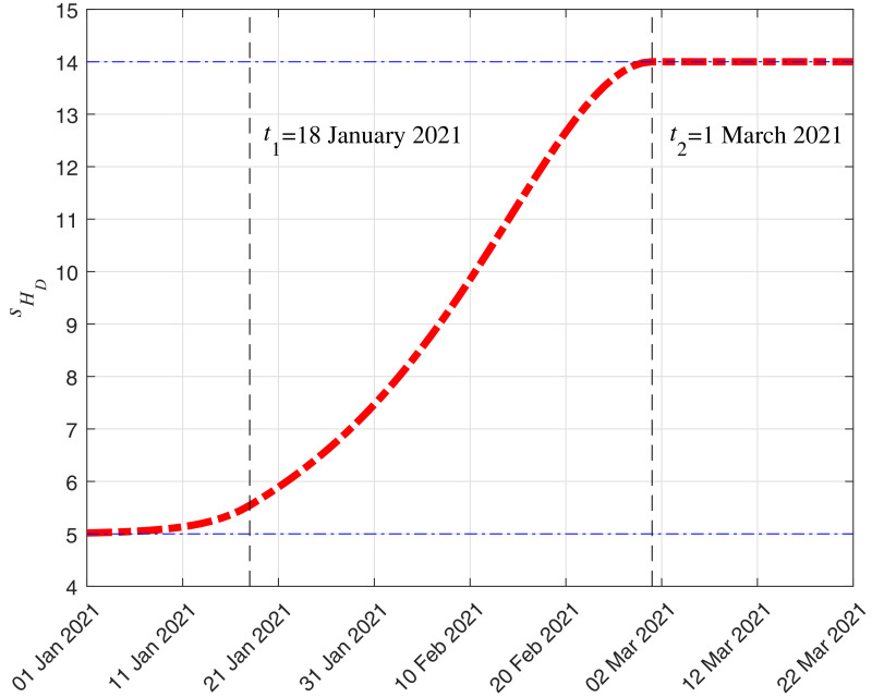
• 5.Update of${\gamma }_{H_D}$: According to the official Italian situation report published on 1 March 2021 (see [26]), the average time (considering the whole amount of reported cases) between hospitalization and death has increased with respect to the previous report published the 16 December 2020. Thus, to simulate this increase, we consider that ${\gamma }_{H_D}\left(t\right)=\frac{1}{5}$ (days${}^{-1}$) when $t$ is before $t_1=$18 January 2021 (we remind that we used official data reported up to 17 January 2021 for the initial submission of this paper), ${\gamma }_{H_D}\left(t\right)=\frac{1}{14}$ (days${}^{-1}$) when $t$ is after $t_2=$1 March 2021, and it increases linearly between those two dates. This particular function provides a good fitting between the reported and simulated deaths.
  Then, following the notation in Remark 3, the mean duration in compartment $H_D$ of an individual that enters that compartment at time $z$ is

  $$s_{H_D}\left(z\right)=5(1-e^{-\frac{T_1}{5}})+e^{\frac{-9/140}{42}{(z+T_1-t_1)}^2}{\int }_{T_1}^{T_2}{e}^{-(\frac{-9/140}{42}{(z+s-t_1)}^2+\frac{s}{5})}\mathrm{d}s+14e^{\frac{-9/140}{42}({(z+T_1-t_1)}^2-{(z+T_2-t_1)}^2)-\frac{T_2}{5}},$$

  where $T_1=\max (0,t_1-z)<T_2=\max (0,t_2-z)$. In Fig. 13 , we show the evolution of the mean duration $s_{H_D}\left(z\right)$ depending on $z$ from $t_0=$ 1 January 2021.

  We point out that this is taken into account in the computation of $t_{H_D}^{\left(i\right)}$, which is used to obtain $R_{\mathrm{e}}^{\left(i\right)}\left(t\right)$, as explained in Remark 3, and $\theta \left(t\right)$, as explained in Section 2.

• 6.Update of$p_{\mathrm{v}}^{\left(2\right)}$: Since we assume in this Annex that, as said above, ${\omega }^{\left(2\right)}=(1+k_{\omega }){\omega }^{\left(1\right)}\ne {\omega }^{\left(1\right)}$, when computing $\theta$ using (5) we need an estimation of $p_{\mathrm{v}}^{\left(2\right)}\left(t\right)$. According to [28], the cases due to the new variant represent 17.8% of the total detected cases in Italy on 5 February 2021, 54% on 18 February, 86.7% on 18 March and 91.6% on 15 April. Furthermore, we assume that there were no cases due to the new variant before 8 October 2020 and that the new variant will represent 99% of the new detected cases on 31 August 2021. Hence, we obtain $p_{\mathrm{v}}^{\left(2\right)}\left(t\right)$ by interpolating all those data using a piecewise cubic Hermite interpolating polynomial.
• 7.Update of the vaccination campaign data: We have updated the data used in the model to simulate the Italian vaccination campaign. Here, we use the new data and estimations reported by the authorities, which have changed with respect to the information available when sending the initial version of this article. More precisely:
  We use the official reported data of the administered doses of the four vaccines used in Italy (Comirnaty, Moderna, Vaxzevria and Janssen) until 24 May 2021. From 25 May 2021 to 31 August 2021, Italy will receive new amounts of doses of these vaccines6 . Besides, they aim to vaccinate 0.5M people per day (see [47]). Considering the data in [9] and [48] and the unused doses from previous months, we summarize the amount of available doses of each vaccine in Table 2 .

  Table 2.

  Estimation of the available doses in Italy from December 2020 to August 2021, according to [9] and [48].

  	From		From			From
  	27 December 2020		25 May 2021			1 July 2021
  	to 24 May 2021		to 30 June 2021			to 31 August 2021
  Vaccine	Available	Used	New available	Total${}_1$	Useda	New available	Total${}_2$
  Comirnaty	22.14M	21.72M	19.28M	19.7M	10.26M	21.02M	30.46M
  Moderna	3.37M	2.69M	2.09M	2.78M	1.44M	9.31M	10.64M
  Vaxzevria	7.38M	6.53M	5.33M	6.18M	3.22M	17.34M	20.3M
  Janssen	0.72M	0.44M	6.59M	6.87M	3.58M	10.63M	13.92M
  Total${}_{\text{Total}}$	33.61M	31.38M	33.29M	35.53M	18.5M	58.3M	75.32M

  ^a

  This column is based on the assumption that the Italian authorities will vaccinate 0.5M people per day and each vaccine contributes with a weight proportional to the amount of available doses, i.e., $500,000\times {\text{Total}}_l/{\text{Total}}_{\text{Total}}$, $l\in \{1,2\}$, per day.
  Furthermore, to estimate the number of people that get or lose immunity after getting the $j$-th vaccine, in this Annex we use the more precise formula (4) instead of (3), with $t_{R_{\mathrm{d}}}=135$ days (see [27]). Therefore, we define functions $u_i$, $i\in \{1,2,3,4\}$ as follows:

  • •
    Comirnaty vaccine: Since the second dose is administered 21 days after the first one, we define:

    $$u_1\left(t\right)=\{\begin{array}{cc}\text{Official}\text{data}\text{from}\text{[9]},\hfill & \text{if}t<25\text{May}\text{2021},\hfill \\ {\displaystyle \max (500,000\frac{19.7}{35.53}-u_1(t-21),0),}\hfill & \text{if}25\text{May}\text{2021}\le t\le 30\text{June}\text{2021},\hfill \\ {\displaystyle \max (500,000\frac{30.46}{75.32}-u_1(t-21),0),}\hfill & \text{if}\text{1}\text{July}\text{2021}\le t\le \text{31}\text{August}\text{2021},\hfill \end{array}$$

    where $e_1$ is given by (11) and (4) may be rewritten in this case as

    $$\begin{array}{ccc}\hfill v_1^{*}\left(t\right)& =& 0.524u_1(t-12)\frac{A_S(t-12)}{F(t-12)}+(0.905-0.524)u_1(t-21)\frac{A_S(t-21)}{F(t-21)}\hfill \\ & & +(0.948-0.905)u_1(t-28)\frac{A_S(t-28)}{F(t-28)}.\hfill \end{array}$$
  • •
    Moderna vaccine: Since the second dose is administered 28 days after the first one, we define:

    $$u_2\left(t\right)=\{\begin{array}{cc}\text{Official}\text{data}\text{from}\text{[9]},\hfill & \text{if}t<25\text{May}\text{2021},\hfill \\ {\displaystyle \max (500,000\frac{2.78}{35.53}-u_2(t-28),0),}\hfill & \text{if}25\text{May}\text{2021}\le t\le 30\text{June}\text{2021},\hfill \\ {\displaystyle \max (500,000\frac{10.64}{75.32}-u_2(t-28),0),}\hfill & \text{if}1\text{July}\text{2021}\le t\le 31\text{August}\text{2021},\hfill \end{array}$$

    where $e_2$ is given by (13) and (4) may be rewritten in this case as.

    $$\begin{array}{ccc}\hfill v_2^{*}\left(t\right)& =& 0.545u_2(t-7)\frac{A_S(t-7)}{F(t-7)}+(0.943-0.545)u_2(t-14)\frac{A_S(t-14)}{F(t-14)}\hfill \\ & & +(1-0.943)u_2(t-28)\frac{A_S(t-28)}{F(t-28)}-(1-0.941)u_2(t-42)\frac{A_S(t-42)}{F(t-42)}.\hfill \end{array}$$
  • •
    Vaxzevria vaccine: Since the second dose is administered 84 days after the first one (see [56]), we define:

    $$u_3\left(t\right)=\{\begin{array}{cc}\text{Official}\text{data}\text{from}\text{[9]},\hfill & \text{if}t<25\text{May}\text{2021},\hfill \\ {\displaystyle \max (500,000\frac{6.18}{35.53}-u_3(t-84),0),}\hfill & \text{if}25\text{May}\text{2021}\le t\le 30\text{June}\text{2021},\hfill \\ {\displaystyle \max (500,000\frac{20.3}{75.32}-u_3(t-84),0),}\hfill & \text{if}1\text{July}\text{2021}\le t\le 31\text{August}\text{2021}.\hfill \end{array}$$

    For this vaccine, we consider the following efficacy function:

    $$e_3\left(s\right)=\{\begin{array}{cc}0,\hfill & \text{if}0\le s<22\text{days},\hfill \\ 0.77,\hfill & \text{if}22\text{days}\le s<31\text{days},\hfill \\ 0.73,\hfill & \text{if}31\text{days}\le s<61\text{days},\hfill \\ 0.78,\hfill & \text{if}61\text{days}\le s<91\text{days},\hfill \\ 0.82,\hfill & \text{if}91\le s,\hfill \end{array}$$

    which corresponds to values for the Vaxzevria vaccine efficacy deduced from [56] (as warned previously in the case of the other vaccines, these values must be taken with caution). Then, the $e_3$ derivative in the distributional sense is

    $${\dot{e}}_3\left(s\right)=0.77\delta (s-22)-(0.77-0.73)\delta (s-31)+(0.78-0.73)\delta (s-61)+(0.82-0.78)\delta (s-91)$$

    and (4) may be rewritten in this case as

    $$\begin{array}{ccc}\hfill v_3^{*}\left(t\right)& =& 0.77u_3(t-22)\frac{A_S(t-22)}{F(t-22)}-(0.77-0.73)u_3(t-31)\frac{A_S(t-31)}{F(t-31)}\hfill \\ & & +(0.78-0.73)u_3(t-61)\frac{A_S(t-61)}{F(t-61)}+(0.82-0.78)u_3(t-91)\frac{A_S(t-91)}{F(t-91)}.\hfill \end{array}$$
  • •
    Janssen vaccine: Since only one dose is administered, we define:

    $$u_4\left(t\right)=\{\begin{array}{cc}\text{Official}\text{data}\text{from}\text{[9]},\hfill & \text{if}t<25\text{May}\text{2021},\hfill \\ {\displaystyle 500,000\frac{6.87}{35.53},}\hfill & \text{if}25\text{May}\text{2021}\le t\le 30\text{June}\text{2021},\hfill \\ {\displaystyle 500,000\frac{13.92}{75.32},}\hfill & \text{if}1\text{July}\text{2021}\le t\le 31\text{August}\text{2021}.\hfill \end{array}$$

    For this vaccine, according to [7], we consider the following efficacy:

    $$e_4\left(s\right)=\{\begin{array}{cc}0,\hfill & \text{if}0\le s<15\text{days},\hfill \\ 0.663,\hfill & \text{if}15\text{days}\le s.\hfill \end{array}$$

    Then, the derivative in the distributional sense of the efficacy function $e_4$ is

    $${\dot{e}}_4\left(s\right)=0.663\delta (s-15),$$

    and (4) may be rewritten in this case as

    $$v_4^{*}\left(t\right)=0.663u_4(t-15)\frac{A_S(t-15)}{F(t-15)}.$$

Fig. 12.

Evolution of $c_{\omega }\left(t\right)$ and $c_{{\beta }_H}\left(t\right)$ from 27 December 2020 to 31 August 2021.

Fig. 13.

Evolution in time of $s_{H_D}\left(z\right)$ (days), which is the mean duration in compartment $H_D$ of an individual that enters that compartment at time $z$, from 1 January 2021.

In Fig. 14, we show some results corresponding to four different scenarios up to 31 August 2021 (of course, many other possibilities could be simulated, including the possibility of new more dangerous variants):

• •Red scenario: The control measures of 11 May 2021 are maintained without changes.
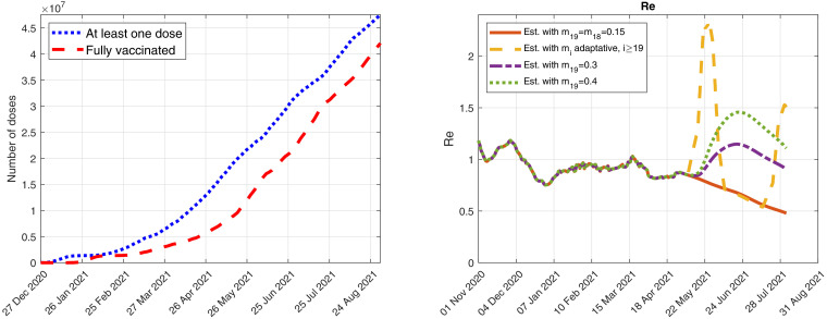
• •Yellow scenario: It simulates an adaptative implementation of the control measures based on the 14-day cumulative incidence, defined by $(c_{\mathrm{m}}\left(t\right)-c_{\mathrm{m}}(t-14))100000/N$, for $t>14$, where $c_{\mathrm{m}}\left(t\right)$ is the model cumulative number of COVID-19 detected cases at day $t$. If the cumulative incidence estimated by the model exceeds 250, then restrictive measures are applied with an intensity of $m=0.15$ and an efficiency of $\kappa =62.0015$. When the cumulative incidence goes below 150, then relaxation measures are implemented with an intensity of $m=0.5$ and the same efficiency of $\kappa =62.0015$. Those threshold values for the cumulative incidence are inspired by the Italian Government indicators described in the Italian official bulletins reported in [25].
• •Purple scenario: The control measures are relaxed from 26 May 2021 considering an intensity of $m=0.3$ and an efficiency of $\kappa =0.0362$.
• •Green scenario: The control measures implemented from 26 May 2021 assume a higher relaxation with an intensity of $m=0.4$ and an efficiency of $\kappa =0.0362$.

In Fig. 15, we include the daily detected cases and deaths caused by each variant for the adaptative scenario (yellow scenario). We also show the cumulative incidence and the effective reproduction numbers obtained by the model.

In Fig. 16 , we include the number of people who received, at least, one dose of any of the four COVID-19 vaccines and also the number of people who have been fully vaccinated against COVID-19, i.e., they have received either one dose of the Janssen vaccine or two doses of the Comirnaty, Moderna or Vaxzevria vaccines7 .

Fig. 16.

Outputs obtained when simulating possible future scenarios described in the Annex. Left: number of people who received, at least, one dose of any of the four COVID-19 vaccines and also number of people who have been fully vaccinated against COVID-19. Right: Evolution of the effective reproduction numbers for the four scenarios studied here.

References

- 1.Baden L.R. The New England journal of medicine. 2020. Efficacy and safety of the mRNA-1273 SARS-CoV-2 Vaccine. [DOI] [PMC free article] [PubMed] [Google Scholar]; https://www.nejm.org/doi/full/10.1056/NEJMoa2035389
- 2.Brauer F., Castillo-Chávez C. Texts in applied mathematics. Springer; 2001. Mathematical models in population biology and epidemiology. [Google Scholar]; https://www.springer.com/gp/book/9781441931825
- 3.Castillo-Laborde C., de Wolff T., Gajardo P., Lecaros R., Olivar G., Ramirez H.. Assessment of event-triggered policies of nonpharmaceutical interventions based on epidemiological indicators. 2020. https://arxiv.org/abs/2011.01036. [DOI] [PMC free article] [PubMed]
- 4.Centers for Disease Control and Prevention, 2020. https://www.cdc.gov/coronavirus/2019-ncov/more/science-and-research/scientific-brief-emerging-variants.html, 30 December.
- 5.Centers for Disease Control and Prevention. COVID-19 vaccines. 2020a. https://www.cdc.gov/coronavirus/2019-ncov/vaccines/index.html, 31 December. [PubMed]
- 6.Centers for Disease Control and Prevention. Implications of the emerging SARS-cov-2 variant VOC 202012/01. 2020b. https://www.cdc.gov/coronavirus/2019-ncov/more/scientific-brief-emerging-variant.html, 22 December. [PubMed]
- 7.Centers for Disease Control and Prevention. Johnson & johnson’s janssen COVID-19 vaccine overview and safety. 2021. https://www.cdc.gov/coronavirus/2019-ncov/vaccines/different-vaccines/janssen.html, 31 March.
- 8.Centers for Disease Control and Prevention. Pfizer-BioNTech COVID-19 Vaccine. 2020c. https://www.cdc.gov/vaccines/covid-19/info-by-product/pfizer/index.html, 30 December.
- 9.Commissario straordinario per l’emergenza Covid-19. Open data su consegna e somministrazione dei vaccini anti COVID-19 in italia. https://github.com/italia/covid19-opendata-vaccini.
- 10.European Centre for Disease Prevention and Control. COVID-19 vaccination and prioritisation strategies in the EU/EEA. 2020a. https://www.ecdc.europa.eu/sites/default/files/documents/COVID-19-vaccination-and-prioritisation-strategies.pdf, 22 December.
- 11.European Centre for Disease Prevention and Control. Key aspects regarding the introduction and prioritisation of COVID-19 vaccination in the EU/EEA and the UK. 2020b. https://www.ecdc.europa.eu/sites/default/files/documents/Key-aspects-regarding-introduction-and-prioritisation-of-COVID-19-vaccination.pdf, 26 October.
- 12.European Centre for Disease Prevention and Control. Risk related to spread of new SARS-CoV-2 variants of concern in the EU/EEA. 2020c. https://www.ecdc.europa.eu/sites/default/files/documents/COVID-19-risk-related-to-spread-of-new-SARS-CoV-2-variants-EU-EEA.pdf, 29 December.
- 13.European Medicines Agency. EMA recommends COVID-19 Vaccine Moderna for authorisation in the EU. 2021. https://www.ema.europa.eu/en/news/ema-recommends-covid-19-vaccine-moderna-authorisation-eu, 6 January.
- 14.Davies N.G., Barnard R.C., Jarvis C.I., Kucharski A.J. MedRxiv. 2020. Estimated transmissibility and severity of novel SARS-CoV-2 Variant of Concern 202012/01 in England. [DOI] [Google Scholar]; https://www.medrxiv.org/content/10.1101/2020.12.24.20248822v1.full
- 15.European Medicines Agency. COVID-19 vaccine moderna. 2020. https://www.ema.europa.eu/en/medicines/human/summaries-opinion/covid-19-vaccine-moderna, December.
- 16.Food and Drug Administration, Moderna COVID-19 vaccine. 2020a. https://www.fda.gov/emergency-preparedness-and-response/coronavirus-disease-2019-covid-19/moderna-covid-19-vaccine, December.
- 17.Food and Drug Administration, Pfizer-bioNTech COVID-19 vaccine. 2020b. https://www.fda.gov/emergency-preparedness-and-response/coronavirus-disease-2019-covid-19/pfizer-biontech-covid-19-vaccine, December.
- 18.Giordano G., Blanchini F., Bruno R., et al. Modelling the COVID-19 epidemic and implementation of population-wide interventions in Italy. Nature Med, 2020. 10.1038/s41591-020-0883-7. [DOI] [PMC free article] [PubMed]
- 19.Giornale di Brescia. Covid: vaccino moderna, entro febbraio 764mila dosi in italia, 9 january 2021. 2021. https://www.giornaledibrescia.it/italia-ed-estero/covid-vaccino-moderna-entro-febbraio-764mila-dosi-in-italia-1.3541432, 9 January.
- 20.GISAID. Tracking of variants. 2021. https://www.gisaid.org/hcov19-variants/.
- 21.Italiano G.. Coronavirus, le misure adottate dal Governo. 2021. https://www.governo.it/it/coronavirus-misure-del-governo, April.
- 22.Hodcroft E.B., CoVariants. SARS-cov-2 mutations and variants of interest. 2021. https://covariants.org/.
- 23.Horby P. NERVTAG paper. 2021. Update note on B.1.1.7 severity. [Google Scholar]; https://assets.publishing.service.gov.uk/government/uploads/system/uploads/attachment_data/file/961042/S1095_NERVTAG_update_note_on_B.1.1.7_severity_20210211.pdf, 11 February
- 24.ore I.s. Prime dosi gi la prossima settimana. 2021. Coronavirus, via libera dell’aifa al vaccino moderna. [Google Scholar]; https://www.ilsole24ore.com/art/coronavirus-via-libera-dell-aifa-vaccino-moderna-prime-dosi-gia-prossima-settimana-ADW8IBCB?refresh_ce=1, 7 January
- 25.Istituto Superiore di Sanitá . URL to Bulletin from 16 December. 2020. Epidemia COVID-19, aggiornamento nazionale. [Google Scholar]; https://www.epicentro.iss.it/coronavirus/bollettino/Bollettino-sorveglianza-integrata-COVID-19_16-dicembre-2020.pdf
- 26.Istituto Superiore di Sanitá . Report based on available data on March 1st. 2021. Characteristics of SARS-cov-2 patients dying in italy. [Google Scholar]; https://www.epicentro.iss.it/en/coronavirus/bollettino/Report-COVID-2019_1_march_2021.pdf
- 27.Istituto Superiore di Sanitá Indicazioni ad interim sulle misure di prevenzione e controllo delle infezioni da SARS-cov-2 in tema di varianti e vaccinazione anti COVID-19. Versione del 13 marzo. 2021 [Google Scholar]; https://www.iss.it/documents/20126/0/Rapporto+ISS+COVID-19+n.+4_2021d.pdf/5ece92de-7793-5f04-4edb-26762a55b47b?t=1615996998754
- 28.Istituto Superiore di Sanitá. Ufficio stampa. primo piano. URL to CS n. 11/2021 - covid-19, in italia il 17.8% delle infezioni dovute a “variante inglese”. ???? https://www.iss.it/primo-piano/-/asset_publisher/3f4alMwzN1Z7/content/id/5622430. URL to CS N. 14/2021 - In Italia il 54% delle infezioni dovute a “variante inglese”, il 4.3% a quella “brasiliana” e lo 0.4% a quella “sudafricana”: https://www.iss.it/primo-piano/-/asset_publisher/3f4alMwzN1Z7/content/id/5647546. URL to CS N. 20/2021 - Covid-19: in Italia la “variante inglese” all 86.7% Il 4.0% dei casi con quella “brasiliana”: https://www.iss.it/web/guest/primo-piano/-/asset_publisher/3f4alMwzN1Z7/content/id/5683229. URL to CS N. 24/2021 - Covid-19: in Italia la “variante inglese” all 91.6%. Il 4.5% dei casi con quella “brasiliana”: https://www.iss.it/primo-piano/-/asset_publisher/3f4alMwzN1Z7/content/id/5714341.
- 29.Ivorra B., Ferrández M.R., Vela-Pérez M., Ramos A.M. Mathematical modeling of the spread of the coronavirus disease 2019 (COVID-19) taking into account the undetected infections. the case of China. Commun Nonlinear Sci Numer Simul. 2020;88:105303. doi: 10.1016/j.cnsns.2020.105303. [DOI] [PMC free article] [PubMed] [Google Scholar]
- 30.Ivorra B., Ngom D., Ramos A.M. Stability and sensitivity analysis of be-codis, an epidemiological model to predict the spread of human diseases between countries. Validation with data from the 2014-16 West African Ebola Virus Disease epidemic Electronic Journal of Differential Equations. 2020;(62):1–29. [Google Scholar]; https://ejde.math.txstate.edu/Volumes/2020/62/ivorra.pdf
- 31.Ivorra B., Ramos A.M., Ngom D. Be-CoDiS: a mathematical model to predict the risk of human diseases spread between countries. Validation and application to the 2014 Ebola Virus Disease epidemic. Bull Math Biol. 2015;77(9):1668–1704. doi: 10.1007/s11538-015-0100-x. [DOI] [PubMed] [Google Scholar]
- 32.Kang S.J., Jung S.I. Age-related morbidity and mortality among patients with COVID-19. Infect Chemother. 2020;52(2):154–164. doi: 10.3947/ic.2020.52.2.154. [DOI] [PMC free article] [PubMed] [Google Scholar]
- 33.Kubik A.B. Parameter estimation for a mathematical model predicting the COVID-19 spread in the área metropolitana de barcelona. Ms Thesis. 2020 [Google Scholar]; https://upcommons.upc.edu/handle/2117/328166
- 34.Mahase E. What have we learnt about the new variant in the UK? BMJ. 2020;371(m4944) doi: 10.1136/bmj.m4944. [DOI] [PubMed] [Google Scholar]
- 35.Ministero della Salute. COVID-19: Il dipartimento scientifico militare del celio ha sequenziato i virus di un soggetto positivo con stessa variante riscontrata in gran bretagna. 2020b. http://www.salute.gov.it/portale/nuovocoronavirus/dettaglioComunicatiNuovoCoronavirus.jsp?lingua=italiano&id=5713, 20 December.
- 36.Ministero della Salute. COVID-19, speranza: “firmata ordinanza per blocco voli dalla gran bretagna”. 2020c. http://www.salute.gov.it/portale/nuovocoronavirus/dettaglioNotizieNuovoCoronavirus.jsp?lingua=italiano&menu=notizie&p=dalministero&id=5228, 21 December.
- 37.Ministero della Salute. Report vaccini anti COVID-19. 2021a. https://www.governo.it/it/cscovid19/report-vaccini/.
- 38.Ministero della Salute. Vaccine day il 27 dicembre in tutta italia e in europa. 2020d. http://www.salute.gov.it/portale/news/p3_2_1_1_1.jsp?lingua=italiano&menu=notizie&p=dalministero&id=5242#:~:text=Ministero%20della%20Salute&text=Il%2027%20dicembre%20in%20tutta%20Italia%2C%20cos%C3%AC%20come%20in%20tutta, all’ospedale%20Spallanzani%20di%20Roma, 26 December.
- 39.Ministero della Salute. Vaccine day, Speranza: ”á il giorno che aspettavamo da tempo. la strada á ancora lunga, ma finalmente abbiamo il vaccino”. 2020e. http://www.salute.gov.it/portale/nuovocoronavirus/dettaglioNotizieNuovoCoronavirus.jsp?lingua=italiano&menu=notizie&p=dalministero&id=5243, 27 December.
- 40.Ministero della Salute. Vaccinazione anti-SARS-cov-2/COVID-19 piano strategico. 2020f. https://www.vaccinarsinsardegna.org/assets/uploads/files/378/piano-strategico-vaccinazione-anti-covid19.pdf.
- 41.Ministero della Salute. Covid-19, speranza firma due ordinanze su misure di contenimento e gestione emergenza. 2021b. http://www.salute.gov.it/portale/nuovocoronavirus/dettaglioNotizieNuovoCoronavirus.jsp?lingua=italiano&menu=notizie&p=dalministero&id=5301, 1 February.
- 42.New and Emerging Respiratory Virus Threats Advisory Group meeting. NERVTAG meeting on SARS-cov-2 variant under investigation VUI-202012/01. 2020. https://khub.net/documents/135939561/338928724/SARS-CoV-2+variant+under+investigation%2C+meeting+minutes.pdf/962e866b-161f-2fd5-1030-32b6ab467896?t=1608470511452, 18 December.
- 43.Our World in Data. Coronavirus (COVID-19) Vaccinations. 2021a. https://ourworldindata.org/covid-vaccinations, January.
- 44.Our World in Data. COVID-19: stringency index. 2021b. https://ourworldindata.org/grapher/covid-stringency-index?tab=chart&country=~ITA, 23 April.
- 45.Pfizer News. Pfizer and bioNTech conclude phase 3 study of COVID-19 vaccine candidate, meeting all primary efficacy endpoints. 2020. https://www.pfizer.com/news/press-release/press-release-detail/pfizer-and-biontech-conclude-phase-3-study-covid-19-vaccine, 18 November.
- 46.Dipartimento della Protezione CivileDati COVID-19 Italiahttps://github.com/pcm-dpc/COVID-19.
- 47.Presidenza del Consiglio dei Ministri. Piano vaccinale antiCOVID, 2021http://www.governo.it/sites/governo.it/files/210313_Piano_Vaccinale_marzo_2021_1.pdf, 13 March.
- 48.Presidenza del Consiglio dei Ministri. Tabella vaccini antiCOVID. aggiornamento 23 aprile 2021. 2021. https://www.salute.gov.it/imgs/C_17_pagineAree_5452_13_file.pdf, 23 April.
- 49.Polack F.P. Safety and efficacy of the BNT162b2 mRNA covid-19 vaccine. N Engl J Med. 2020;383:2603–2615. doi: 10.1056/NEJMoa2034577. [DOI] [PMC free article] [PubMed] [Google Scholar]
- 50.Public Health England PHE monitoring of the effectiveness of COVID-19 vaccination. Impact COVID-19 vaccines Mortalit England. 2021 [Google Scholar]; https://www.gov.uk/government/publications/phe-monitoring-of-the-effectiveness-of-covid-19-vaccination
- 51.Ramos A.M. Editorial Complutense. 2012. Introducción al análisis matemático del método de elementos finitos. [Google Scholar]; ISBN (paper book): 9788499381282. ISBN (e-book): 9788499381299
- 52.Ramos A.M., Ferrández M.R., Vela-Pérez M., Kubik A.B., Ivorra B. A simple but complex enough -SIR type model to be used with COVID-19 real data. Application to the case of italy. Physica D: Nonlinear Phenomena. 2020;421:132839. doi: 10.1016/j.physd.2020.132839. [DOI] [PMC free article] [PubMed] [Google Scholar]; http://www.doi.org/10.1016/j.physd.2020.132839
- 53.Reyna-Lara A., Soriano-Paños D., Gómez S., Granell C., Matamalas J.T., Steinegger B., Arenas A., Gómez-Gardeñes J. Virus spread versus contact tracing: two competing contagion processes. Phys Rev Res. 2021;3(1):013163. doi: 10.1103/PhysRevResearch.3.013163. [DOI] [Google Scholar]
- 54.TG24 S.. Vaccino anti covid: da moderna 47mila dosi da lunedá ecco quante ne arriveranno in totale. 2021. https://tg24.sky.it/salute-e-benessere/2021/01/10/vaccino-anti-covid-dosi#00, 10 January.
- 55.Virological.org. Preliminary genomic characterisation of an emergent SARS-cov-2 lineage in the UK defined by a novel set of spike mutations. 2020. https://virological.org/t/preliminary-genomic-characterisation-of-an-emergent-sars-cov-2-lineage-in-the-uk-defined-by-a-novel-set-of-spike-mutations/563, 19 December.
- 56.Voysey M. Single-dose administration and the influence of the timing of the booster dose on immunogenicity and efficacy of chadox1 ncov-19 (AZD1222) vaccine: a pooled analysis of four randomised trials. THE LANCET. 2021;397:881–891. doi: 10.1016/S0140-6736(21)00432-3. [DOI] [PMC free article] [PubMed] [Google Scholar]
- 57.Wise J. Covid-19: new coronavirus variant is identified in UK. BMJ. 2020;371(m4857) doi: 10.1136/bmj.m4857. [DOI] [PubMed] [Google Scholar]; https://doi.org/10.1136/bmj.m4857
- 58.World Health Organization. Draft landscape of COVID-19 candidate vaccines. 2020b. https://www.who.int/publications/m/item/draft-landscape-of-COVID-19-candidate-vaccines, 29 December.
- 59.World Health Organization. SARS-cov-2 variant united kingdom of great britain and northern ireland disease outbreak news. 2020c. https://www.who.int/csr/don/21-december-2020-sars-cov2-variant-united-kingdom/en/, 21 December.
- 60.World Health Organization. Weekly epidemiological update - 19 January 2021. 2021. https://www.who.int/publications/m/item/weekly-epidemiological-update---19-january-2021, 19 January.
Associated Data
This section collects any data citations, data availability statements, or supplementary materials included in this article.
Data Availability Statement