Isogeometric finite element-based simulation of the aortic heart valve: Integration of neural network structural material model and structural tensor fiber architecture representations

Abstract

The functional complexity of native and replacement aortic heart valves are well known, incorporating such physical phenomenons as time-varying non-linear anisotropic soft tissue mechanical behavior, geometric non-linearity, complex multi-surface time varying contact, and fluid-structure interactions to name a few. It is thus clear that computational simulations are critical in understanding AV function and for the rational basis for design of their replacements. However, such approaches continued to be limited by ad-hoc approaches for incorporating tissue fibrous structure, high-fidelity material models, and valve geometry. To this end, we developed an integrated tri-leaflet valve pipeline built upon an isogeometric analysis (IGA) framework. A high-order structural tensor (HOST) based method was developed for efficient storage and mapping the two-dimensional fiber structural data onto the valvular 3D geometry. We then developed a neural network (NN) material model that learned the responses of a detailed meso-structural model for exogenously cross-linked planar soft tissues. The NN material model not only reproduced the full anisotropic mechanical responses but also demonstrated a considerable efficiency improvement, as it was trained over a range of realizable fibrous structures. Results of parametric simulations were then performed, as well as population based bicuspid aortic heart valve fiber structure, that demonstrated the efficiency and robustness of the present approach. In summary, the present approach that integrates HOST and NN material model provides an efficient computational analysis framework with increased physical and functional realism for the simulation of native and replacement tri-leaflet heart valves.

1. INTRODUCTION

1.1. The native and replacement aortic heart valve

Functionally, the aortic heart valve (AV) is a tri-leaflet structure that ensures unidirectional blood flow between the left ventricle and aorta. Along with the pulmonary heart valve, it is often termed a ‘semi-lunar’ valve due to the characteristic shape of the leaflets. The AV is primarily a passive soft tissue structure in that it responds to local hemodynamic forces and changes in aortic root diameter over the cardiac cycle. However, this apparently simple purpose does not adequately describe the complexity of its physiological function. The AV’s underlying mechanical function is multi-modal, multi-scale, and repeated every second of life to a total of approximately three billion times in the course of a typical lifetime. In spite of this staggering level of durability, almost 300,000 heart valve surgeries are performed annually world-wide [1]. Of these, a majority of the replacements are for the treatment of calcific aortic valve disease, which is an active multi-factorial degenerative process [2,3,4]. In addition to the general population, approximately 2% of the US population have the bicuspid aortic valve (BAV) congenital anomaly. In this pathology, a pair of AV leaflets are fused to varying degrees, while the remaining leaflet can be distorted. In reality, the BAV pathology is a continuous range of malformations that range from a single leaflet to four (quadcusp). Irrespective of the exact anatomy, just the presence of BAV is an important risk factor for aortic stenosis.

Regardless of the underlying causes, the primary treatment for AV disease remains replacement with an artificial valve, with current clinical approaches using a bioprosthetic heart valve (BHV) [5,6]. BHV are a tri-leaflet design with leaflets fabricated from xenograft pericardial biomaterials. Use of BHV continues to increase worldwide [7,8, 9], largely due to the development of percutaneous BHV designs that are emerging as an alternative to standard surgical designs [6,10]. In general, it is expected that this new technology will rapidly develop, especially in the elderly population, which has a higher operative risk. However, BHV durability continues to remain limited to the range of 10–15 years; often achieved only in patient ages 57 years or older.

1.2. Tri-leaflet valve simulation-based studies

Overall, rigorous simulation with the objective of complementing exploratory experimentation and technological invention will be crucial to the development of BHV designs. This is a daunting challenge; both the native and replacement aortic heart valve are functionally complex, incorporating such physical phenomenons as non-linear anisotropic soft tissue mechanical behavior, geometric non-linearity, complex contact, and fluid-structure interactions. It is thus no surprise that that computational simulations are critical in understanding their function and for the rational basis for the development of improved replacement valves. Indeed, computational simulations, either alone or in conjunction with clinical studies, have been used to define how evolving biomechanical properties drive native heart valve disease as well as replacement valve function and performance [11]. Many groups have approached heart valve simulations, with a focus such important aspects as high-fidelity time-evolving material modeling, patient specific geometries, and fluid-structure interactions [11,12,13,14,15].

Yet, despite these substantial advancements in simulation technology and its implementation, critical issues remain in the simulation of native and replacement heart valves. This is due to the fact that, ironically, while heart valves are essentially fluidic components, the mechanisms of their pathologies and degeneration lie mainly in the behaviors of the constituent cells and tissues. Thus, while organ level simulations can assist in understanding how the valve dynamically responds over the cardiac cycle, leaflet tissue remodeling, degeneration, and ultimately failure are a direct result of our poor understanding of the underlying processes. In the long term, these processes need to be understood, quantified, modeled mathematically, and ultimately incorporated into organ and system level simulations [16,17]. Moreover, means to systematically integrate organ-level geometric features with finer structures (e.g local fiber architecture) are still typically performed in an ad-hoc manner with varying degrees of fidelity.

1.3. Key simulation advancements needed for more realistic and robust AV simulations

1.3.1. AV leaflet fiber architecture representations

Both native and bioprosthetic AV leaflets are composed of layered soft tissues mainly composed of collagen fibers. The fibrous architecture thus dictates the direction and degree of mechanical anisotropy, as well as the overall elastic responses [18,19]. This is especially the case in diseased states. As an example, we have quantified the structure of human normal and bicuspid AV leaflets in the early disease stage [20]. The regularity in the observed of the fibrous structure in the measured population was a surprising finding. It suggested that consistent population based tissue structural metrics for the human BAV population exist and could potentially be used for patient specific simulations. However, such information is generally experimentally obtained as a two dimensional (2D) field of excised valve tissues using point-wise probability orientation distribution functions (ODFs). To be useful in a simulation context, such information must be mapped from the 2D in-vitro measurement state to the in-vivo 3D leaflet geometry. The ODF mapping methods should be efficient and completely generalized; allowing for rotations, translations, and affine deformation-based transformations. Moreover, newer measurement methods such as polarized spatial frequency domain imaging, have pixel-level resolution and can generate gigabytes of structural information for a single leaflet alone [21,22]. There is thus a need to develop efficient storage and rapid mapping techniques to transfer of high resolution in-vitro derived collagen fiber ODFs to the 3D leaflet surface geometry.

1.3.2. Use of machine learning in high-fidelity material modeling in finite element analyses

An often overlooked, critical limitation we address herein for AV simulations is their substantial computational cost. This is particularly important in practical applications where patient specific pipelines that involve complex multiple surgical outcome scenarios need to be explored in clinically relevant time-frames. The same is true in earlier design stages to explore various, including patient specific, valve designs rapidly. This situation becomes particularly acute when the modeled material responses go beyond basic elastic responses to simulate more complex time-dependent phenomena, such as tissue remodeling or leaflet biomaterial fatigue. As an example, we have recently developed a detailed, microstructurally based mechanism underlying the BHV fatigue process [23]. To model the permanent set effect, we assume that the exogenously crosslinked matrix undergoes changes in its reference configurations over time. The changes in the collagen fiber architecture due to dimensional changes allowed us to predict subsequent changes in mechanical response. However, the mathematical formulation contains double and quadruple integrals, making it computationally intractable as-is. We developed an effective constitutive model which can fully reproduce the response of a wide range of planar soft tissues [24]. While this approach preformed well in a variety of heart valve simulations, its response time was still too long to be usable in rapid calculations. This is in part due to the fact that the effective model parameters needed to be refit for each change in the microstructural model at each successive time point. Thus, while effective constitutive modeling approaches and related model reduction methods can significantly improve the computational efficiency and numerical robustness of multi-scale and meso-scale models, these approaches remain too computationally expensive for extensive parametric studies or high speed clinical usage.

One approach to address these issues is the use of machine learning model representations of the material models themselves. The most popular approach has been the use of neural networks (NN). This approach has a long and rich history, including such application areas as elastomeric foams [25], fiber reinforced polymeric composites [26], and fatigue modeling. In most of these approaches, the analytical model is replaced with an NN representation [27,28], and an autoprogressive method is then used for training NNs to learn complex stress-strain behaviour of materials using load-deflection response measured in experimental structural tests [29]. NNs represent an exciting branch of computational science as they have shown an ability to reproduce the behaviors of many complex systems efficiently, often with substantial performance enhancements over other established methods. Yet, while able to reproduce experimental findings, current NN approaches are dependent on an extensive and appropriate experimental database, which is not always available or even practically obtainable. The underlying physical mechanisms are also lost, as well as mathematical issues such as convexity are not necessarily guaranteed. Clearly, while NNs offer great potential for advanced material modeling, they need to be incorporated into simulation pipelines in way that preserves and extends our physical understanding of the underlying mechanisms, along with the appropriate mathematical constraints.

1.3.3. Attribute-rich NURBS based methods for geometric description and finite element analyses.

Interest in parametric studies of native and replacement heart valve leaflet geometry dates back to at least Thubrikar [30] and later Reul [31]. More contemporary approaches based on non-uniform rational B-splines (NURBS) [32] offers greater flexibility to perform both parametric and patient-specific parametric studies. Further, the use of NURBS has allowed for direct integration into finite element (FE) solvers using isogeometric analysis (IGA) [33,34,35,36]. The use of IGA is of particular importance as shell elements are typically used to represent the leaflets, and IGA provides a very smooth representation ideal for leaflet accurate contact simulations. NURBS-based approaches also have a largely untapped capability to store and spatially map scalar, vector, and tensor fields as attributes directly onto the AV geometry. For example, material model parameters (which can vary point wise) and the fibrous architectures from individual [37] or more recently population based data [20] are just a few of the examples. The recent availability of population based data is of particular interest for mapping, as one can typically obtain high resolution patient specific geometry but not other detailed attributes. Thus, the ability to spatially map population-derived attributes to patient specific geometries remains a largely unmet need.

1.4. Study organization

As a step towards addressing the above issues, we have developed an integrated tri-leaflet valve simulation pipeline built upon an IGA framework, which allowed for a unified description of geometry that readily integrated application-specific attributes. In brief, a high-order structural tensor (HOST) based method was developed for efficient storage and mapping the fiber structure onto the valvular geometry. We then developed a neural network material model that learned the responses of a detailed meso-structural model for exogenously cross-linked heart valve leaflet tissues, which is more complex than the responses of native tissues that also relies on the fiber dispersion (splay) and can be learned using the same approach. We opted for use of this tissue model as opposed to our native tissue, with no loss of generality, as we were also interested replacement heart valve applications which utilize cross-linked pericardial tissues. We then demonstrated the efficacy of this using detailed parametric studies, along with invivo derived bicuspid aortic heart valve fiber structure. We organized the manuscript as follows. Given the necessary length of the developmental aspects of this work, we present methods and intermediate results for each major step first, followed by a formal Results section of the key parametric studies of the fully development model. A detailed discussion is then presented, along with necessary appendices.

2. METHODS

2.1. Study overview

In the present study we have developed a comprehensive pipeline that addresses the above issues (fig. 1) that includes the following major components:

Fig. 1:

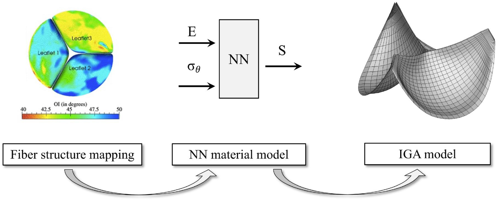
A schematic of the computational pipeline for integrated IGA-based model utilizing the NN material model and tensor-mapped fiber structure

1. Development of a HOST method to represent fiber ODFs. This approach allows for efficient storage and representation, as well as tensor coordinate transformation methods to facilitate mapping to the NURBS based geometric representations of heart valve leaflet geometry.

2. Development of a finite element implementation of an NN representation of structural constitutive model for native and cross-linked tissues[23]. This approach allows for direct simulation of the full range of fiber architecture that can predict the resultant tissue stress-strain responses, without the need for evaluation of multiple integrals or parameter refitting for different structures at run-time.

3. Integration of the HOST mapping and NN-based material model into an integrated AV IGA-based model, all built in the the Unified Form Language of the FEniCS open source package [38].

4. Demonstration of the efficacy of the approach in parametric studies, as well as using human derived, population-based normal and BAV leaflet data [20].

Details are presented in the following sections.

2.2. The structural constitutive model for native and xenograft heart valve tissues

Material modeling of soft tissues has a long rich history, and includes a wide variety of biomedical applications [39]. As in many applications, heart valve tissues phenomenological approaches can mathematically relate stress and strain states with good accuracy [40]. Yet, there is a more critical aspect of tissue modeling which involves the underlying mechanisms of growth, remodeling, and degeneration in both native and bioprosthetic heart valve tissues. For example, there is evidence that vavlular tissues undergo plastic deformation. An important finding is that the underlying collagen fiber architecture has a limiting effect on the maximum changes in geometry that the permanent set effect can induce. Thus, our group’s approach has been to take a structural approach to elucidate and simulate the underlying mechanisms [18].

We start by reviewing the formulation of a recently developed structural constitutive model for native and xenograft heart valve tissues, as described in detail in [41,23,24], which forms the rationale for the development of the methods developed herein. In brief, the constitutive model assumes that the total tissue strain energy Ψ is the summed contributions from the collagen fibers Ψ_col, fiber-fiber interactions Ψ_int, and the non-fibrous matrix Ψ_mat. Assuming incompressiblity due to the high water content, this yields

$$\Psi ={\varphi }_{\text{mat}}{\Psi }_{\text{mat}}+{\varphi }_{\text{col}}{\Psi }_{\text{col}}+{\varphi }_{\text{col}}{\Psi }_{\text{int}}-p(J-1),$$ (1)

where ϕ_mat is the mass fraction of matrix, ϕ_col is the mass fraction of the collagen fibers, the scalar p is the indeterminate Lagrange multiplier, and J = det(F), where F is the deformation gradient tensor. Note that for non-crosslinked (native) tissues no fiber-fiber interactions are assumed to occur, so that Ψ_int = 0. The specific form of Ψ_i for each model component i (i = mat, col, int) are given as follows. For the matrix contribution Ψ_mat a modified Yeoh model is used

$${\Psi }_{mat}=\frac{{\eta }_{\text{mat}}}{2}\left(\frac{1}{a}{\left(I_1-3\right)}^a+\frac{r}{b}{\left(I_1-3\right)}^b\right), \text{with} 1<a<b,ab<2,r\ge 0.$$ (2)

Here, η_mat is the modulus parameter, I₁ is the first invariant of the right Cauchy-Green deformation tensor C = F^TF, a, b are the shape parameters, and r is the weight between the two terms. For the collagen fibers Ψ_col is an ensemble average over the fiber orientation distribution function Γ, and the recruitment distribution function, Γ_s, i.e.,

$${\Psi }_{\text{col}}={\eta }_{\text{col}}{\int }_{\theta }\Gamma (\theta ){\int }_1^{{\lambda }_{\theta }}{\Gamma }_s\left({\lambda }_s\right){\left(\frac{{\lambda }_{\theta }}{{\lambda }_s}-1\right)}^2\text{d}{\lambda }_s\text{d}\theta .$$ (3)

where, η_C is the modulus of the collagen fibers, ${\lambda }_{\theta }=\sqrt{\theta \cdot C\cdot \theta }$ is the stretch in θ direction, λ_s is the slack stretch, and λ_θ/λ_s is the true stretch after collagen fibers are straightened. In a similar fashion, the interaction term, Ψ_int, is an ensemble level term integrated over all possible pairs ensembles

$${\Psi }_{\text{int }}=\frac{{\eta }_{\text{int }}}{2}{\int }_{\alpha }{\int }_{\beta }\Gamma (\alpha )\Gamma (\beta ){\int }_1^{{\lambda }_{\alpha }}{\int }_1^{{\lambda }_{\beta }}{\Gamma }_s\left(x_{\alpha }\right){\Gamma }_s\left(x_{\beta }\right){\left(\frac{{\lambda }_{\alpha }{\lambda }_{\beta }}{x_{\alpha }{x}_{\beta }}-1\right)}^2\text{d}{x}_{\alpha }\text{d}{x}_{\beta }\text{d}\alpha \text{d}\beta .$$ (4)

We assumed that the tissue incompressibility is determined solely by the matrix phase. To determine the expression for the second Piola-Kirchhoff stress tensor S, we utilized $S=2\frac{\partial \Psi (C)}{\partial C}-p{C}^{-1}$. The resulting complete expression for $2\frac{\partial \Psi (C)}{\partial C}$ is given by

$$2\frac{\partial \Psi (C)}{\partial C}={\varphi }_{\text{mat}}{\eta }_{\text{mat}}\left({\left(I_1-3\right)}^{a-1}+r{\left(I_1-3\right)}^{b-1}\right)\left(I-C_{33}{C}^{-1}\right)+{\varphi }_{\text{col}}{\eta }_c{\int }_{\theta }\Gamma (\theta )\left({\int }_1^{{\lambda }_{\theta }}\frac{{\Gamma }_s(x)}{x}\left(\frac{1}{x}-\frac{1}{{\lambda }_{\theta }}\right)\text{d}x\right)\left(n_{\theta }\otimes n_{\theta }\right)\text{d}\theta +{\varphi }_{\text{col}}{\eta }_{\text{int}}{\int }_{\alpha }{\int }_{\beta }\Gamma (\alpha )\Gamma (\beta )\left(\sum _{i\in \{\alpha ,\beta \}}\frac{n_i\otimes n_i}{{\lambda }_i}{\int }_1^{{\lambda }_{\alpha }}{\int }_1^{{\lambda }_{\beta }}\frac{2{\lambda }_{\beta }{\Gamma }_s\left(x_{\alpha }\right){\Gamma }_s\left(x_{\beta }\right)}{x_{\alpha }{x}_{\beta }}{\left(\frac{{\lambda }_{\alpha }{\lambda }_{\beta }}{x_{\alpha }{x}_{\beta }}-1\right)}^2\text{d}{x}_{\alpha }\text{d}{x}_{\beta }+\sum _{i,j\in \{\alpha ,\beta \},i\ne j}\frac{n_i\otimes n_i}{{\lambda }_i}{\int }_1^{{\lambda }_j}{\Gamma }_s\left(x_j\right){\left(\frac{{\lambda }_j}{x_j}-1\right)}^2\text{d}{x}_j\right)\text{d}\alpha \text{d}\beta ,$$ (5)

while the Lagrange multiplier p for the incompressibility constraint can be determined by the plane stress condition. It should be noted that the coupling term in eqn. 5 is a relatively new addition to this class of models and has been shown to be required by chemically cross-linked tissues such as the pericardial xenograft tissues used in BHV, as well as more structurally complex tissues such as myocardium [42]. More importantly, while both accurate and predictive, eqn. 5 as presented remains impractical for high speed computational simulations.

2.3. HOST: High Order Structural Tensors to represent in planar fiber orientation distributions

Introduction.

As underscored in the preceding section, fibrous structures play an important role in the function and mechanical behavior of soft biological tissues [39]. Moreover, imaging technologies have now progressed to the point where very high density information (e.g. at the pixel level) can be acquired in near real-time on soft tissue fibrous structure [22,21,43]. This represents an unprecedented opportunity to further develop computational modeling approaches for soft tissue structures that incorporate such high-fidelity structural information in the underlying constitutive models. This is especially the case where disease or damage has occurred, where the local structural can be quite complex (e.g. [44,20]).

However, such information is typically acquired as 2D maps of excised, flattened tissues, and thus cannot be directly used in 3D geometries. Mathematically, the planar fiber orientation distribution function is represented as Γ(X, n), which describes the probability of the relative number of fibers at a position X having an orientation described by the unit vector n, with $X,n\in {ℝ}^2\left({\Vert n\Vert }_2=1\right)$. In general, Γ(X, n) will need to be translated and rotated from the 2D measurement to the 3D surface. In addition to these rigid body transformations, mapping will also need to include incorporation in-surface stretch and compression to account for the in-vivo pre-strains known to exist in native valve tissues [45,46], which are released when the tissue is excised prior to 2D mapping measurements. Moreover, we seek to develop a method for efficient storage, as newer imaging methods for structural analysis can produce gigabytes of data for a single leaflet [22].

To summarize, we seek to develop an efficient means to represent and transform high-fidelity structural information for FE model development, which includes the following major goals:

1. A means for efficient storage and representation.

2. A means to facilitate translation, rotation, and in-surface deformations associated from the 2D data to the 3D leaflet surfaces. This should include both geometries used for data acquisition (e.g. the unloaded state) and remapped (e.g. when the data was acquired in a loaded configuration but needs to be mapped back to the reference state, as in [47]). Note that the affine transformation has been shown to be valid in native heart valve tissues [48]).

3. Integrate as an attribute attached to NURBS-based geometric representations.

We present our methodology in the following.

Basic characteristics of Γ.

We start by establishing the basic characteristics of Γ. It should be noted that the following can also be utilized for single and multiple layered tissue models, such as the that developed for the mitral valve [19]. Due to the inherent symmetries in any fiber ODF, Γ will be a symmetric function of n so that

$$\Gamma (n)=\Gamma (-n).$$ (6)

Taking advantage of this relation, we further define n = n(θ) with θ ∈ Ω = [−π/2, π/2]. The normalization requirement of an ODF thus requires

$${\int }_{\Omega }\Gamma [n(\theta )]\text{d}\theta =1.$$ (7)

From Γ, several key fiber orientation characteristics can be derived. The preferred fiber direction, θ_p, is determined using

$${\theta }_p={\int }_{\Omega }\Gamma [n(\theta )]\theta \text{d}\theta .$$ (8)

High order structural tensor representations

Structural tensors have a long history in the analysis of texture in materials, with general frameworks formulated for a wide range materials for 3D distributions based on spherical harmonics [49] and planar distributions using Fourier series [49,50]. In the present work, we specialize these approaches for planar soft tissue representations, with an emphasis on efficient representation and tensor coordinate transformation to facilitate the mapping process. Lower rank (n=4) structural tensors have been used for several micro-mechanical applications (e.g. [50]). While a 4th rank approach will work for mildly aligned fibrous tissues, they perform poorly for much more aligned fibrous architectures. To develop the method for higher rank representations of Γ, we start with the following truncated Fourier series representation

$$\Gamma [n(\theta )]=\frac{1}{2\pi }\left[1+\sum _{j=1}^7{a}_{2j}cos(2j\theta )+b_{2j}sin(2j\theta )\right],$$ (9)

where a_i and b_i are constants determined using standard methods. We note that an upper harmonic limit of j = 7 was found to be more than sufficient to capture highly aligned soft tissue fiber orientation distribution behaviors (Figure 2).

Fig. 2:

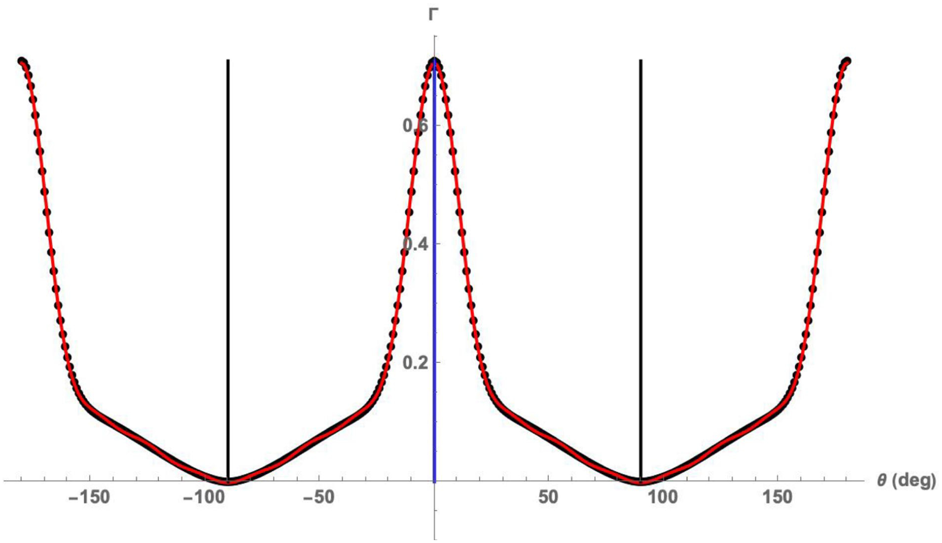
Example of the 14th rank structural tensor fit to Γ from the anterior leaflet of the mitral valve, showing an excellent fit. Also shown are the axes of symmetry as determined by eigenvectors of second rank structural tensor $D_{i_1,i_2}$. The blue and black lines represent angular locations of the first and second eigenvectors, respectively, of the second rank deviator tensor $D_{i_1,i_2}$. These eigenvectors define the local preferred e_PD and cross-preferred e_XD fiber (unit vector) directions, respectively.

Next, we introduce an m^th rank deviator tensor $D_{i_1,i_2,\dots ,i_m}$, which is a fabric tensor of the third kind [49]. $D_{i_1,i_2,\dots ,i_m}$ has a number of favorable mathematical properties, such as

$$\begin{gathered} D_{i,j}=D_{j,i} \\ {D}_{i,j,k,l}=D_{j,i,k,l}=D_{k,i,j,l}=D_{l,i,j,k}=D_{k,l,i,j},\dots \\ {D}_{i,i}=1 \\ {D}_{i,j}=D_{i,j,k,k}, \end{gathered}$$ (10)

with the summation convention enabled. It can be shown for any order m that certain components of $D_{i_1,i_2,\dots ,i_m}$ are directly related to Fourier coefficients a_i and b_i in eqn. 9 using

$$D_{i_1,i_2,\dots ,i_m}=\{\begin{array}{l}{(-1)}^{k/2}{a}_{m}k:\text{ even }\hfill \\ {(-1)}^{(k-1)/2}{b}_{m}k:\text{ odd }\hfill \end{array}$$ (11)

where k is the number of value “2” indices. All other remaining coefficients can be determined by symmetry using eqn. 10. For example, the 4th rank $D_{i_1,i_2,i_3,i_4}$ has only five independent components determined directly from the Fourier coefficients. (Table 1). Similar expressions can be obtained for $D_{i_1,i_2,\dots ,i_m}$ for any rank m. Once the components of $D_{i_1,i_2,\dots ,i_m}$ are established, Γ can then be easily recovered, with D₀=1 to satisfy the normalization requirement in eqn. 7, using

$$\Gamma (n)=\frac{1}{2\pi }\left(1+D_{i_1,i_2}{n}_{i_1}{n}_{i_2}+D_{i_1,i_2,i_3,i_4}{n}_{i_1}{n}_{i_2}{n}_{i_3}{n}_{i_4}+\cdots +D_{i_1,i_2\dots i_m}{n}_{i_1}{n}_{i_2}\dots n_{i_m}\right).$$ (12)

where Einstein summation convention is used for contractions over indices i₁, …, i_m and $n_{i_1},\dots ,n_{i_m}$ are the corresponding components of n. When applied to the highly aligned mitral valve leaflet tissue, this approach worked very well (Figure 2). Once Γ is so obtained, it is commonly required to determine the axes of symmetry of Γ as required by the symmetry property (eqn. 6). This is easily done using the eigenvalues of the second rank deviator tensor $D_{i_1,i_2}$, which acts essentially as a low-pass filter. The resulting eigenvectors of $D_{i_1,i_2}$, which indicates the axes of symmetry for Γ, can be physically interpreted as the preferred e_PD and cross-preferred e_XD fiber (unit vector) directions (Fig. 2). When eqn. 12 is truncated to 14th rank structural tensor, only 14 Fourier series coefficients need to be stored for mapping Γ(n) in comparison to the 360 values in the experimental data obtained at each measurement point.

Table 1:

An example showing the five independent component values for a 4^th rank fabric tensor $D_{i_1,i_2,i_3,i_4}$ in terms of the associated Fourier series coefficients.

$D_{i_1,i_2,i_3,i_4}$	k	independent component
D1111	0	a4
D1112	1	b4
D1122	2	−a4
D1222	3	−b4
D2222	4	a4

HOST-based generalized coordinate transformations of Γ.

One major benefit of the HOST approach is that it facilitates generalized coordinate system mapping of Γ. To do this, we represent a coordinate mapping from each point in the reference configuration X₀ to the new mapped configuration X by the deformation gradient tensor F(X₀), where dX = F(X₀) · dX₀ locally under the assumption of affine transformation. This adopted form is a fully generalized mapping approach for planar fibrous structures. To develop the method, Γ is transformed using the following two steps. First, we separate the deformation and rigid body rotation components using the polar decomposition F = R·U, where R are the orthogonal rotation and U the stretch tensors, respectively. We first account for the effects the local stretch U, under the assumption of affine transformation, on Γ in the deformed (but not rotated) state using [51]

$${\Gamma }^{\prime }(n)=\Gamma (n)\frac{n\cdot Cn}{J_{2D}}$$ (13)

where J_2D = det(U) and C = U². Once Γ′ has been determined, the associated transformed Fourier series constants and deviator tensors $D_{i_1,i_2,\dots ,i_m}$ are then determined (see §2.3). Next, to account for the rigid body rotation R, the all deviator tensors are transformed using standard tensor coordinate transformation rules. For example, the 4^th rank fabric tensor expressed in the mapped coordinate system $D_{i_1,i_2,i_3,i_4}^{\prime }$ can be determined using

$$D_{i_1,i_2,i_3,i_4}^{\prime }=R_{i_1,j_1}{R}_{i_2,j_2}{R}_{i_3,j_3}{R}_{i_4,j_4}{D}_{j_1,j_2,j_3,j_4}$$ (14)

and the HOST form in eqn. 12, which is a function of these Fourier coefficients, is used to rotate/distort the Γ(n) when performing the mapping operations to obtain Γ′(n). This is required to map the 2D experimentally acquired Γ(n) data to Γ′(n) on 3D surfaces, such as the 3D heart valve leaflet. Further, distortion is important when trying to account for the effects of tissue contraction after removal from the in-vivo environment. This approach thus produces high-fidelity representations of generalized forms of Γ(n) with only 14 parameters at each data point, as well as facilitating straightforward generalized geometric mapping using only conventional tensor coordinate transformations, which are both easy to use and computationally efficient.

2.4. A machine learning model of native and cross-linked heart valve tissue mechanical behaviors

Background.

To numerically implement the structural model (eqn. 5) using Gaussian quadrature, the quadruple integral of the interaction term alone requires up to 10⁴ quadrature points. This gives rise to the need of a dramatically more computationally efficient approach that can replicate the response of high fidelity structural models. We have explored the use of simplified analytical model forms to avoid the computational demands of the necessary integrations [24]. However, such approaches can reproduce only one state at a time, so that their parameters have to be re-determined for each state change (e.g. change in initial or current fiber orientation). While the high fidelity and physically accurate aspects of the structural approaches remain attractive to make the necessary mechanistic connections, new approaches must thus be developed to address these computational demands.

Our goal herein is thus to develop machine-learning based computational representation of heart valve tissue mechanical behaviors. Our goal was thus not to develop alternative NN based material models but rather efficient computational representations using NN methods. In doing so we avoid constructing NN models directly from raw experimental data. This approach, while popular, often requires a large quantities of data that is typically not available. “Data” is also not necessarily a homogeneous body of information; it is typically dependent on many specific conditions and methods unique to a particular study. Collected data thus may or may not be appropriate for the modeling tasks at hand. There are also mathematical restrictions on the strain energy equivalent of the NN model, such as ellipticity and convexity, that need to be enforced. Moreover, the mechanistic, highly predictive, mature nature of available structural models are an attractive alternative source of material behaviors to be represented.

We thus focus our approach instead on a NN representations of our high fidelity physics-based material model (eqn. 5) for the purpose of computational speed and to facilitate rapid parametric studies. This approach allowed accurate computational representation of the material models that also closely obey various necessary mathematical properties, such as convexity and symmetry (since they are trained on physics models that have these properties). Once the NN model is thus trained, it can replace the original physics-based model in the finite element model under consideration to dramatically speed up subsequent simulations. We detail our approach in the following.

Formulation of a NN model for Ψ_fsm.

For each material point, the mapped Γ was incorporated as follows. e_PD was taken as the local x₁ in the undeformed configuration, e_XD as x₂ to form a Cartesian coordinate system. While the complete Γ is available at each material point using the methods laid out in §2.3, we seek to demonstrate the efficacy of this approach in the present work. Thus, to simplify NN architecture and training, we assumed that the mapped Γ can be represented as a truncated normal distribution ${\mathcal{N}}_{\mathcal{T}}(\theta \mid \mu ,\sigma )$, wherein μ = θ_p so that e_PD = n_p and is aligned to the local x₁ direction, and σ is the standard deviation of Γ. Thus, the local x₁ direction now represents the local dominant (i.e. stiffer) material axial direction. This reduces the Γ mapping to a single local scalar variable σ, which is dispersion of the fiber splay about the local x₁ direction. This allowed use to utilize only a single scalar variable to describe the local Γ.

In the present work, we use the components of the Green-Lagrange strain tensor E referred to the material axes [23]. These are defined using

$$E_{PD}=e_{PD}\cdot E\cdot e_{PD},E_{XD}=e_{XD}\cdot E\cdot e_{XD},E_{\varphi }=e_{PD}\cdot E\cdot e_{XD}.$$ (15)

Since the preferred direction e_PD is aligned with the local coordinate x₁, the NN model only needs to have E_PD, E_XD, E_ϕ, and σ as the inputs, and outputs second Piola-Kirchhoff stress tensor predicted components with respect to the same bases, i.e.,

$$S_{PD}=e_{PD}\cdot S\cdot e_{PD},S_{XD}=e_{XD}\cdot S\cdot e_{XD},S_{\varphi }=e_{PD}\cdot S\cdot e_{XD}.$$ (16)

Thus, the complete forward model of the NN model is denoted as

$$\left(S_{PD},S_{XD},S_{\varphi }\right)=f_{\text{NN}}\left(E_{PD},E_{XD},E_{\varphi },\sigma \right).$$ (17)

which serves as a simulacrum to the structural model (eqn. 5) over the physiological range of σ while other structural parameters are fixed. In both NN model training and parametric studies, by simply varying the local σ, the NN model can predict the range of responses from high anisotropy to nearly isotropy.

To take the advantage of the expressive power of a fully connected NNs were used to approximate the response of the full structural model. Given the fact that the full structural model is differentiable and unbounded, the softplus function $h:ℝ\mapsto ℝ,h(x)=\text{log}\left(1+e^x\right)$ is chosen as the activation function in the NN. The softplus function is a smoothed version of the rectified linear unit (ReLU). In the overall design of the NN, the neurons on the l-th layer $x_l\in {ℝ}^{d_l}\left(l=1,\dots ,n_l\right)$, can be obtained by a composition of an affine transformation A of the neurons on the previous layer, $x_{l-1}\in {ℝ}^{d_{l-1}}$ and the nonlinear activation function h, using

$$x_l=h\circ A\left(x_{l-1}\right)=h\left(W_l\cdot x_{l-1}+b_l\right)$$ (18)

The affine transformation $A:{ℝ}^{d_{l-1}}\mapsto {ℝ}^{d_l}$ is defined by its weights $W_l\in {ℝ}^{d_l\times d_{l-1}}$ and bias $b_l\in {ℝ}^{d_l}$, and the activation function h is applied in an element-wise fashion. The dimension of the output layer $d_{n_l}=3$. The loss function defined later for training the NN is an aggregated quantity which means the NN is driven to minimize the error on average not any particular local misfits. Numerically, the trained NN without such enforcement will output a small but nonzero S_ϕ when E_ϕ = 0, therefore, the third output of the output layer is post-multiplied by the shear strain E_ϕ to enforce the constraint that S_ϕ = 0 when E_ϕ = 0. Steps involved in the computation of (17) is described in Algorithm 1.

Algorithm 1.

The forward model of the NN model with n_l − 1 hidden layers

1: Initialize x0 ← (EPD, EXD, Eϕ, σ)

2: for l = 1 : nl do

3:   xl = h (Wi · xl−1 + bi)

4: (SPD, SXD, Sϕ) ← $\left(x_{n_l,1},x_{n_l,2},x_{n_l,3}\times E_{\varphi }\right)$

5: return (SPD; SXD; Sϕ)

Training NN models for Ψ_fsm and the final NN model form.

The training data were generated by the full structural model eqn. 5 using η_mat = 100 kPa, η_col = 302039.9656 kPa, η_int = 2785.73 kPa, a = 1, b = 1, r = 0. The recruitment distribution Γ_s(λ_s) was kept constant, and was considered independent of θ, in keeping with our other work [41]. To model Γ_s(λ_s), we utilized the following Beta Distribution [41]. First, we map λ_s to the [0, 1] domain

$$y=\frac{{\lambda }_s-{\lambda }_{\text{lb}}}{{\lambda }_{\text{ub}}-{\lambda }_{\text{lb}}},$$

where λ_lb and λ_ub represent the lower and upper bounds, respectively, with values λ_lb = 1.0 and λ_ub = 1.2130. Next, Γ_s(y) is determined using

$${\Gamma }_s(y)=\frac{y^{\alpha -1}{(1-y)}^{\beta -1}}{B(\alpha ,\beta )\left({\lambda }_{\text{ub}}-{\lambda }_{lb}\right)}$$

where α = 8.0525, β = 1.1378, and B(α, β) is a normalization constant that depends on α and β. The training dataset D_tr defined as

$${\mathcal{D}}_{tr}={\left\{\left(E_{PD}^{(i)},E_{XD}^{(i)},E_{\varphi }^{(i)},{\sigma }^{(i)},S_{PD}^{(j)},S_{XD}^{(j)},S_{\varphi }^{(j)}\right)\right\}}_{i=1}^{n_{tr}},$$ (19)

are evenly spaced data points in prescribed bounded ranges, such that $\left(E_{PD}^{(i)},E_{XD}^{(i)},E_{\varphi }^{(i)},{\sigma }^{(i)}\right)\in \left[E_{PD}^{lb},E_{PD}^{ub}\right]\otimes \left[E_{XD}^{lb},E_{XD}^{ub}\right]\otimes \left[E_{\varphi }^{lb},E_{\varphi }^{ub}\right]\otimes \left[{\sigma }^{lb},{\sigma }^{ub}\right]$ for all i = 1, …, n_tr, where n_tr is the number of training points. The range of the training dataset covers the physiologic range in which the deformation of heart valve tissues most likely to occur. We generated n_tr = 11⁴ training data points with the full structural model, using extant parameters for crosslinked bovine pericardium (See §2.2) that were evenly spaced within the bounds $E_{PD}^{lb}=E_{XD}^{lb}=0$, $E_{PD}^{ub}=0.17$, $E_{XD}^{ub}=0.23$, $E_{\varphi }^{ub}=-0.15$, $E_{\varphi }^{ub}=0.15$, σ^lb = 10° and σ^ub = 50° (Fig. 5). Note that the data points with stress components with higher than 1500 kPa are removed since they were considered beyond the physiological range. While we can retain the data points outside the physiological range for training the NN, it will undermine the fitting quality of the NN within the physiological range due to the fact that larger stress values have larger contribution to the relative mean squared error, and can thus skew the trained model.

Fig. 5:

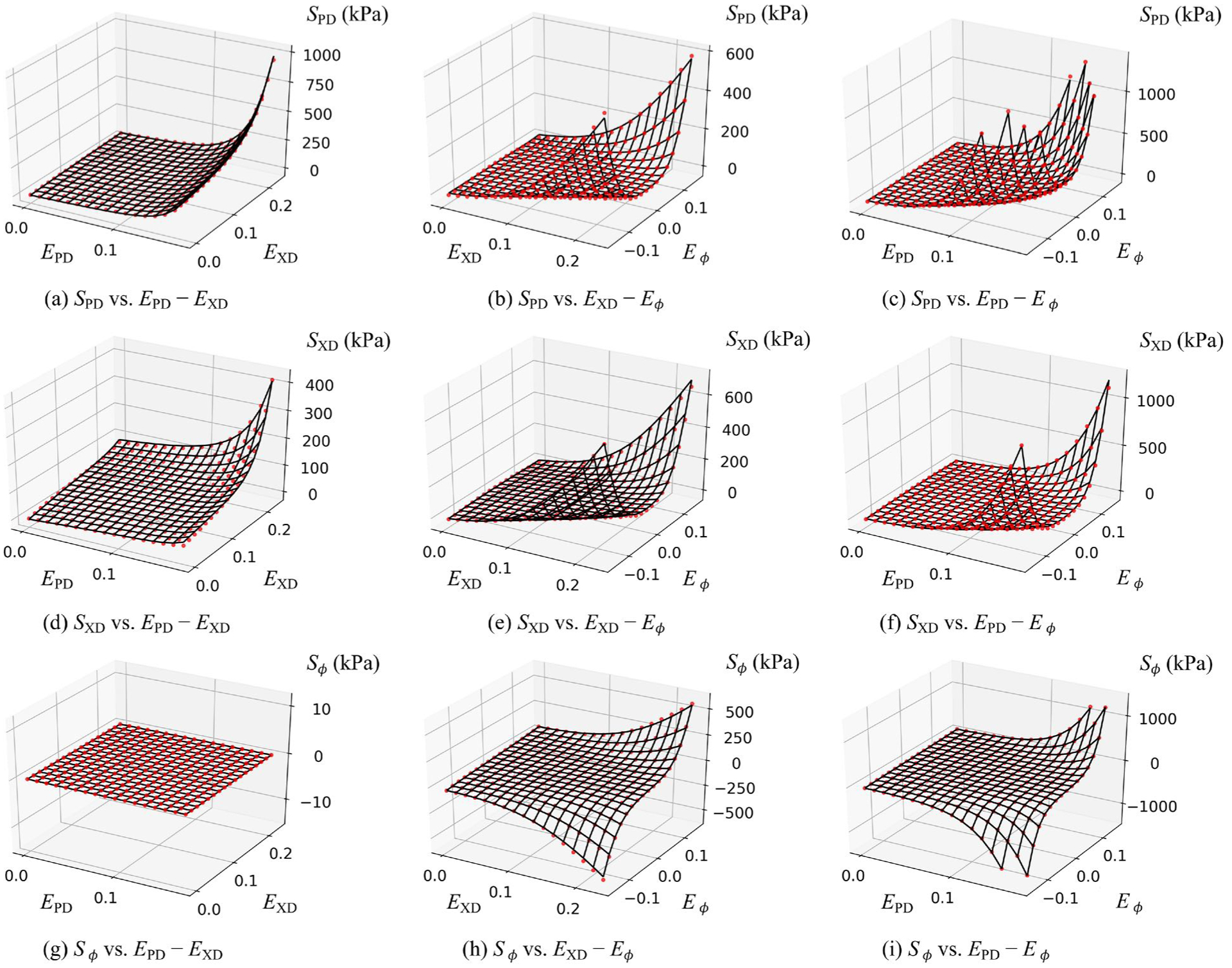
Graphical depiction of the strain ranges used to train the NN model. Also shown are the validation results for the final NN model for σ = 25.48°.

Training for the NN commenced using randomly uniform distributions to initialize NN parameters. The relative mean squared error (MSE) between the predicted stresses of the NN model and those generated by the full structural model, which is defined using

$$e=\frac{{\sum }_{j=1}^n{\Vert f_{\text{NN}}\left(E_{PD}^{(j)},E_{XD}^{(j)},E_{\varphi }^{(j)},{\sigma }^{(j)}\right)-\left(S_{PD}^{(j)},S_{XD}^{(j)},S_{\varphi }^{(j)}\right)\Vert }_2^2}{{\sum }_{j=1}^n{\Vert \left(S_{PD}^{(j)},S_{XD}^{(j)},S_{\varphi }^{(j)}\right)\Vert }_2^2}.$$ (20)

was chosen as the loss function for training the NN model. The training was accomplished strictly offline, thus all training data are generated before parameter optimization. For a faster and stable convergence, the parameters are updated by the limited memory BFGS algorithm. Backpropagation was used to compute the gradient of the loss function with respect to the NN parameters (W_l, b_l for l = 1, …, n_l). The validation data are generated in the same fashion as sampling the training data but do not contain any training data. The relative MSE in eqn. 20 is also used to quantify the fitting quality on validation dataset.

Development of the final form of the NN model.

The observed predictive power of the NN was directly related to the specified complexity of the NN. We thus first trained a number of NNs with different number of hidden layers and neurons on the same training data (Fig. 3). The 1-layer NNs were not able to describe the behavior of the full structural model with given error threshold, while 2-layer or 3-layer NNs had sufficient complexity to replicate the full structural model. In our particular application, there is a trade-off between complexity and efficiency for 2/3-layer NNs. Based on these results, we choose a 2-layer NN model with 10 neurons in each layer, as it was computationally less-expensive than a 3-layer one and yet has similar performance.

Fig. 3:

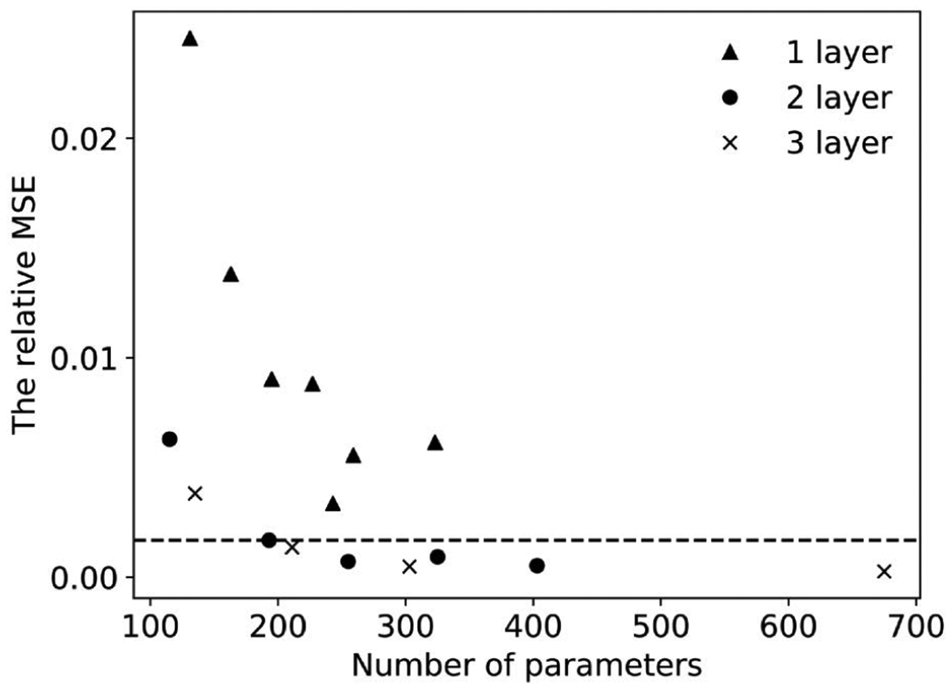
The training error of NNs with different numbers of layers and neurons.

Good convergence characteristics were found for the optimizer for training the NN with 2 × 10 neurons (Fig. 4a). Validation error tests of this model against the full structural model were conducted. We obtained the validation error e_val, given by eqn. 20, on validation data sets with different numbers of samples. Evidently, the relative validation error is around 6e−3 (Fig. 4b). To visualize the validation results, a random σ is selected and then we plot the 3 stress components on 3 strain planes (Fig. 5), which shows that the NN model fitted the full structural model quite well.

Fig. 4:

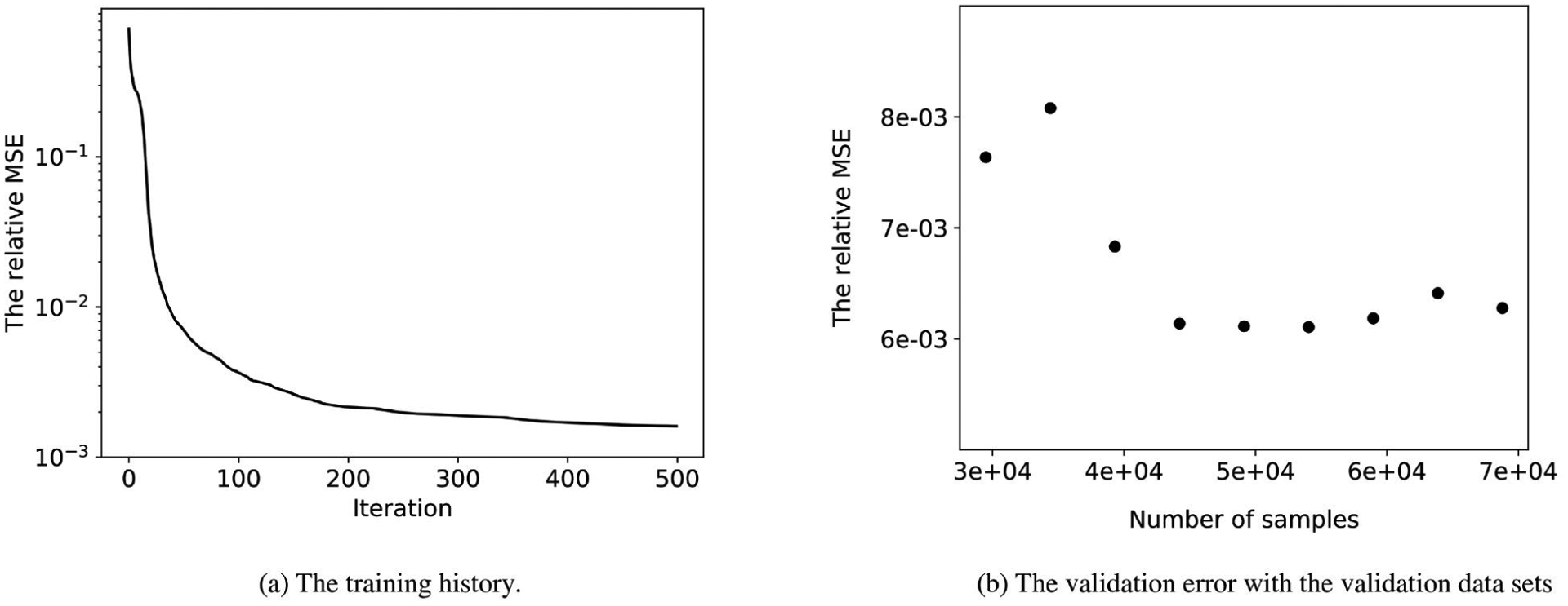
The training history and validation errors of the final NN model with 2 × 10 neurons.

Convexity and related considerations.

A concern when simulating an elastic constitutive model is the convexity of the strain energy function, as well as the positive definiteness and symmetry of the associated elasticity tensor $ℂ=\partial S/\partial E$. In general, while NN’s have the property of being universal approximations of continuous functions, underlying symmetries are not guaranteed to be reproduced exactly. This can be enforced on the DNN by first transforming the inputs to a set of symmetric functions, as for reproducing the symmetry of a strain energy function based on the symmetry group of the material [52].

In the present application, we note that the structural model is intrinsically convex, and the symmetry of the $ℂ$ is merely a consequence of the double derivative of the continuously differentiable strain energy function [53]. Equivalent convexity constraints can be enforced into parameter estimation of alternative conventional models (e.g. [24]) when the mathematical form of the model is simple. Since the present NN model is nonlinear in the parameters, the number of convexity constraints would be as large as the training dataset, and is thus impractical. Thus, in the present NN model the convexity constraint is not explicitly enforced.

To verify that this approach did not appreciably affect simulation accuracy, we calculated the eigenvalues of $ℂ$ in the training dataset. This test demonstrated that 97.7% of the data points have the positive definite stiffness matrix. In the validation dataset, the eigenvalues of $ℂ$ were all real numbers. The $ℂ$ that have negative eigenvalues were located on the boundary of the fitting range, where there are less data points that can regulate the response of the NN model. In all cases the convexity is retained in the interior of the fitting range or physiological range. Additionally, at most only one out of three eigenvalues of each elasticity tensor was negative, and it is significantly smaller than the positive ones. The $ℂ$ of the present NN model is generally not perfectly symmetric [28]. Since the NN is fitted to the stress response, $ℂ$ is expected to have lower order of accuracy than the stress. The resulting effective “numerical” symmetry of $ℂ$ can be measured by the ratio of the squared norm of the symmetric part to the squared norm of the matrices using eqn. 21 using all data points in the test dataset ${\mathcal{D}}_{\mathit{\text{test}}}$. In the present study, we found that the resulting ratio was 97.89%, which meant the symmetric part of $ℂ$ was very dominant. Finally, we note that the NN model (Fig. 6) the third output was post-multiplied with the shear strain E_ϕ, which gives the shear stress S_ϕ, resulting in that zero shear strain gives zero shear stress.

Fig. 6:

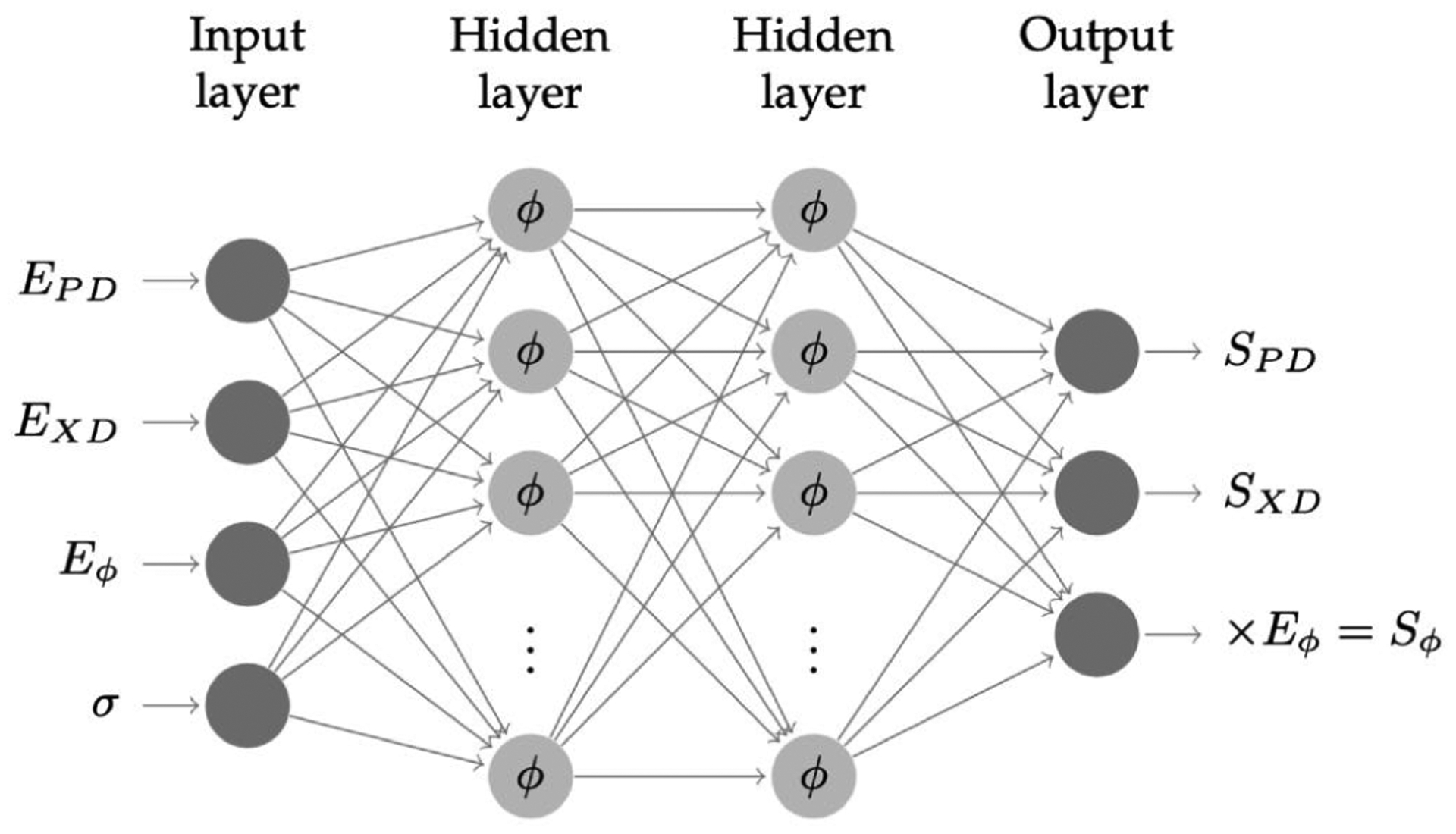
A schematic of the final fully connected NN model for planar mechanical behavior of native and replacement heart valve leaflet soft tissues. The input nodes consist of the strain tensor components and the Γ standard deviation. The output is the three stress tensor components. Note that the shear stress term is post-multiplied with the shear strain, resulting in that zero shear strain gives zero shear stress as fitting constraint (see text for details).

$$r=\frac{{\sum }_{i\in {\mathcal{D}}_{\mathit{\text{test}}}}{\Vert \mathit{\text{symm}}\left(ℂ\left(E^{(i)}\right)\right)\Vert }^2}{{\sum }_{i\in {\mathcal{D}}_{\mathit{\text{test}}}}{\Vert ℂ\left(E^{(i)}\right)\Vert }^2},$$ (21)

2.5. NURBS-based tri-leaflet geometric representation

The methods for the formulation of the NURBS based representation of a tri-leaflet heart valve used in this study has been previously presented [54]. Briefly, starting from the NURBS surface representation of the geometry used in [55], valve leaflets were parametrically designed by picking nine “key points” located on the ends of commissure lines and the bottom of the sinuses. This method was used to parametrically change the free edge and belly curve, and therefore change the valve design to match the shape of the valve taken from [55]. This procedure was implemented in an interactive geometry modeling and parametric design platform based on Rhinoceros 3D and Grasshopper. A NURBS mesh with 20×26 control points is generated for each heart valve leaflet. The NURBS mesh has open uniform knots so that the Dirichlet boundary conditions can be directly imposed by setting the values of corresponding control points. The NURBS mesh is degree 2 in order to give C₁ continuous basis functions for Kirchhoff–Love shell analysis.

We first describe the mid-surface of each leaflet in the reference (undeformed) configuration $X\left({\xi }^1,{\xi }^2\right):{ℝ}^2\mapsto {ℝ}^3$ and current (deformed) configuration $x\left({\xi }^1,{\xi }^2\right):{ℝ}^2\mapsto {ℝ}^3$ are parameterized by ξ¹ and ξ². The covariant basis vectors, and the unit surface normal vector are

$$a_{\alpha }=x_{,\alpha }=\frac{\partial x\left({\xi }^1,{\xi }^2\right)}{\partial {\xi }^{\alpha }},a_3=\frac{a_1\wedge a_2}{{\Vert a_1\wedge a_2\Vert }_2},$$ (22)

$$A_{\alpha }=X_{,\alpha }=\frac{\partial X\left({\xi }^1,{\xi }^2\right)}{\partial {\xi }^{\alpha }},A_3=\frac{A_1\wedge A_2}{{\Vert A_1\wedge A_2\Vert }_2},$$ (23)

where α = 1, 2. To map the 2D fiber coordinate system information defined on 2D excised leaflet $X_0\in {ℝ}^2$ (Fig. 7b) onto the 3D leaflet $X\in {ℝ}^3$ (Fig. 7c), the point correspondence $X\left(X_0\right):{ℝ}^2\mapsto {ℝ}^3$ between them is first established by fitting the NURBS patch to the 2D leaflet triangular mesh (Fig. 7a) where the raw fiber data is stored [20]. The B-Spline mesh (Fig. 7c) has two degenerate points at the left the right corners. For simulation purposes, the NURBS mesh (Fig. 7c) is cropped at the corner of the commissures and annulus to improve the mesh quality with structured quadrilateral elements (Fig. 7d). The leaflet geometry is minimally modified after cropping the corner, and the element quality and the convergence of the simulation are improved. This small change will have limited effect on the simulation results since the geometry is changed minimally. The corresponding pushforward F = ∂X/∂X₀ can be obtained. Given F, the deformed ODFs (eqn. 13) and transformed structural tensor can be obtained. Thus, the preferred direction on the 3D leaflet can be transformed by $e_{PD}=R{e}_{PD}^{2D}$. For simulation purposes, we only need to store its components on the covariant basis of the reference configuration, e_PD = λ₁A₁ + λ₂A₂, ∥e_PD∥₂ = 1 (Fig. 8). The cross direction e_XD (∥e_XD∥₂ = 1) in the tangent space is assumed to be orthogonal to e_PD. Using F = RU, we can via eqn. 14 and recover its corresponding point-wise Γ on the 3D leaflet surface. Note that, in general, R is not enough to transform Γ since the mapping also involves in-surface stretches. As an example, we demonstrate this method using the mapped σ for the normal and bicuspid valves taken from [20] (Fig. 9).

Fig. 7:

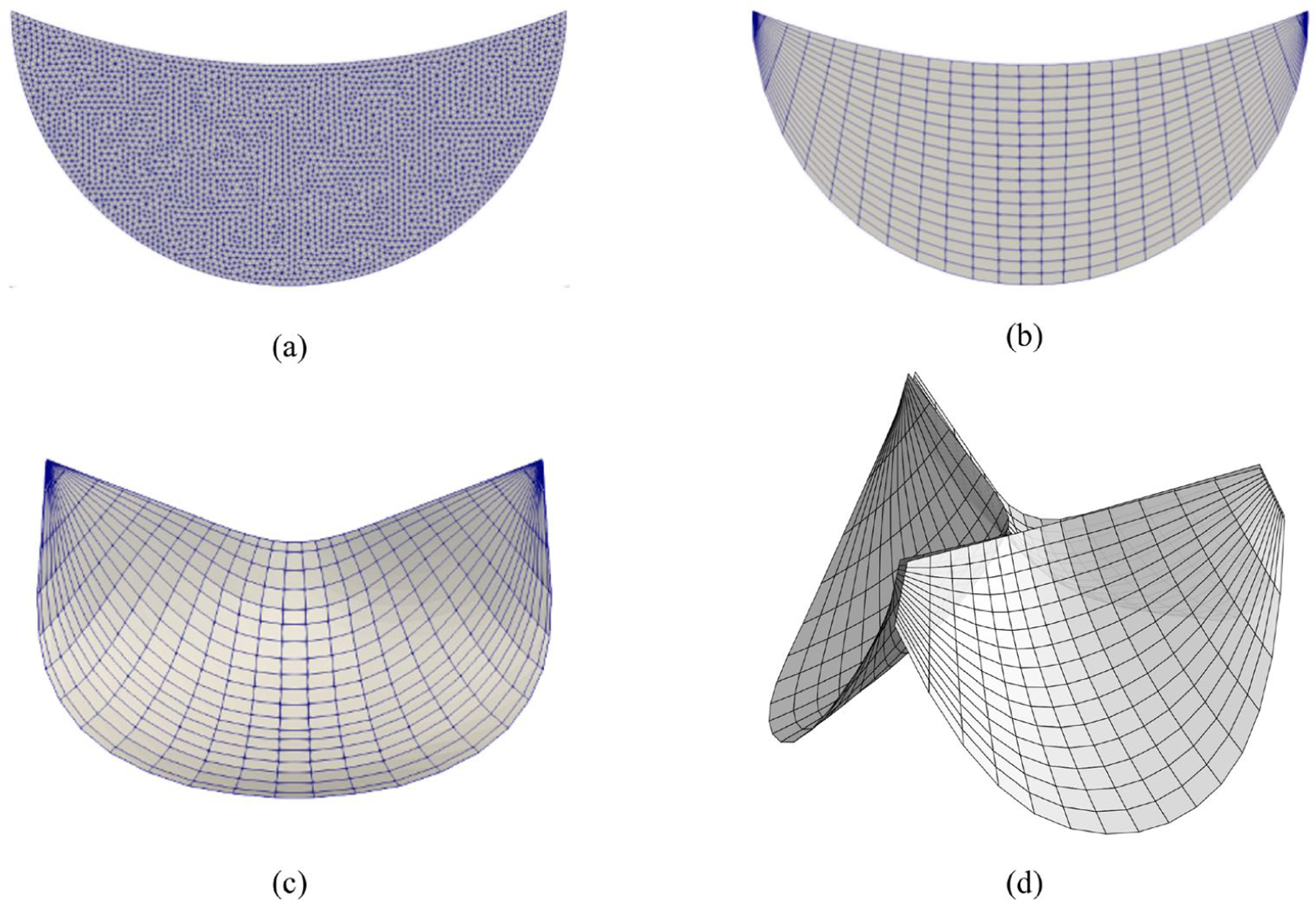
The 2D triangular mesh (a) is first fit by a 2D NURBS mesh (b) to interpolate fiber ODFs on the NURBS mesh. Then the fiber ODFs at a point X₀ on the 2D NURBS mesh can be mapped to the corresponding point X on the 3D leaflet geometry (c). The NURBS mesh (d) for simulations consists of three identical 3D leaflet geometries with cropped corner to improve the mesh quality.

Fig. 8:

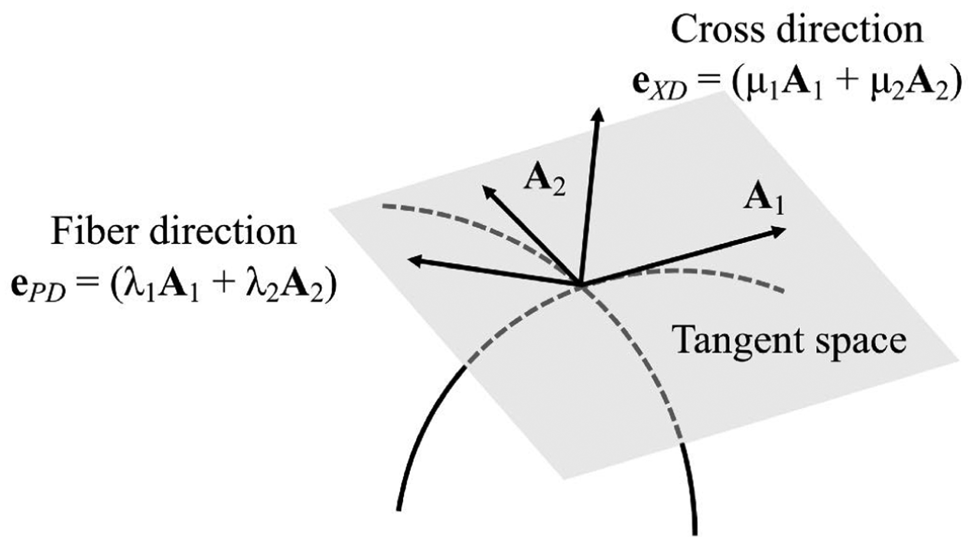
The preferred direction and cross direction defined on the tangent space.

Fig. 9:

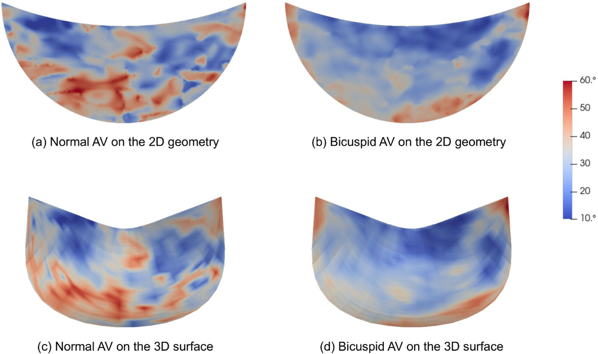
The σ distribution of normal AV (a) and bicuspid AV (b) on the 2D geometries are mapped to (c) and (d) on the 3D NURBS leaflet surfaces, respectively.

2.6. FEniCS isogeometric formulation and implementation

The heart valve finite element implementation was based on related previous studies [54,56]. Briefly, we model heart valve leaflets as thin shells based on the K-L theory. With IGA basis functions, e.g., B-spline, NURBS, the C¹ continuity requirement for the K-L element is easily satisfied. The simulations were implemented with tIGAr [57], which is a Python library for isogeometric analysis (IGA) using FEniCS [38], an open-source finite element (FE) open source software.

FEniCS implementation.

The current and reference configuration x(ξ¹, ξ²) and X(ξ¹, ξ²) of the mid-surface of a leaflet are discretized by IGA basis functions defined on the mesh described in §2.5. The IGA basis functions can be represented by FE basis functions using a global variant of Bézier extraction [57]. This makes it possible to use FEniCS to implement IGA. To illustrate how this is implemented in tIGAr, we consider the homogeneous IGA scalar basis function $N_A^{\text{IGA},\text{hom}}\left({\xi }^1,{\xi }^2\right)$ which can be obtained by a linear transformation M_BA of FE basis functions $N_A^{\text{FE}}\left({\xi }^1,{\xi }^2\right)$ such as Lagrange basis functions,

$$N_A^{\text{IGA},\text{hom}}\left({\xi }^1,{\xi }^2\right)=\sum _B{M}_{BA}{N}_B^{\text{FE}}\left({\xi }^1,{\xi }^2\right).$$ (24)

The rational IGA basis functions can be obtained with

$$N_A^{\text{IGA}}\left({\xi }^1,{\xi }^2\right)=\frac{w_A^{\text{IGA}}{N}_A^{\text{IGA},\text{hom}}\left({\xi }^1,{\xi }^2\right)}{{\sum }_B{w}_B^{\text{IGA}}{N}_B^{\text{IGA},\text{hom}}\left({\xi }^1,{\xi }^2\right)}.$$ (25)

Thus, the current configuration defined by an IGA function $x={\sum }_A{p}_A^{\text{IGA}}{N}_A^{\text{IGA}}$ can be expressed in homogeneous representation, as can the reference configuration $X={\sum }_A{q}_A^{\text{IGA}}{N}_A^{\text{IGA}}$. The covariant basis a_α and A_α can be obtained by eqn. 22 and eqn. 23, respectively.

By the assumption of negligible trough-thickness shear deformations in K-L shells, the covariant basis vectors in the current and reference configuration of the 3D medium of the shell are g_α = a_α + ξ³a_3,α and G_α = A_α + ξ³A_3,α. By the second fundamental form of the surface, we have b_αβ = g₃ · g_α,β and B_αβ = G₃ · G_α,β where

$$g_3=\frac{g_1\wedge g_2}{{\Vert g_1\wedge g_2\Vert }_2},G_3=\frac{G_1\wedge G_2}{{\Vert G_1\wedge G_2\Vert }_2}.$$ (26)

Then, the metric tensors are g = a − 2ξ³b and G = A − 2ξ³B, and the strain is defined as $E_{\alpha \beta }=\frac{1}{2}\left(g_{\alpha \beta }-G_{\alpha \beta }\right)$ in the local in-plane curvilinear system. Given the fiber structure mapping, we can transform E_αβ into E_ij on a local Cartesian system consistent with the material axis e_PD and an orthogonal in-plane direction e_XD. The in plane stresses can be obtained by the NN model with σ, i.e., S = f_NN(E, σ)−pC⁻¹. In the variational problem, the internal virtual work is defined as

$$\delta W_{\text{int}}={\int }_{{\Omega }_0}{\int }_{-h_{th}/2}^{+h_{th}/2}\delta E_{ij}{S}_{ij}\text{d}{\xi }^3\text{d}X.$$ (27)

The Lagrange multiplier p for the incompressible constraint of the matrix material is determined by p = 2C₃₃∂Ψ_mat/∂C₃₃.

2.7. Verification of the full model

We first verified the implementation of the NN material model in planar biaxial test simulations under multiple loading protocols against the mathematical expression of the NN model. The NN model is implemented in FEniCS using UFL (§5.1). A unit square domain is discretized by a 10 × 10 bi-linear quadrilateral mesh. The preferred and cross directions are aligned with the edges of the square. The Dirichlet boundary conditions were uniformly imposed on each edge of the square. The prescribed displacement is imposed according to three different protocols: E_PD : E_XD = 1 : 1, 0.17 : 0.23, and 1 : 3. Since the strains are uniform on the domain, the stress of the IGA simulation is uniform as well. We then verified the stress-strain relationship in FE with that obtained from the NN model in Fig. 10.

Fig. 10:

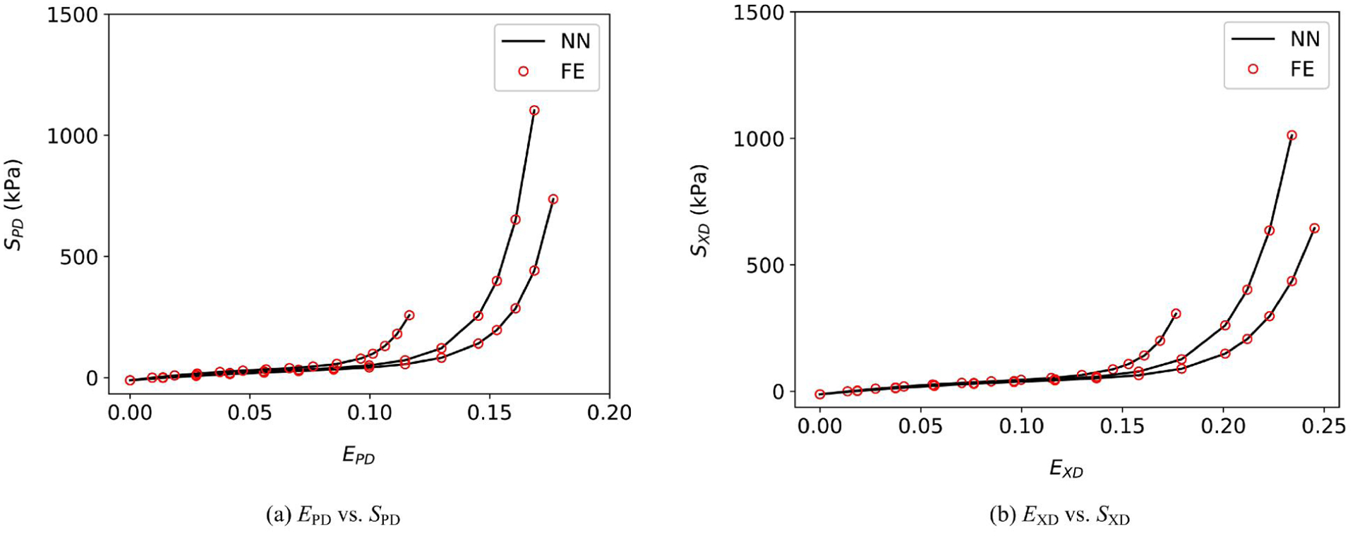
Verification of the FE implementation with the NN model for three planar biaxial test protocols: E_PD : E_XD = 1 : 1, 0.17 : 0.23, 1 : 3.

The full structural model is very accurate and quite predictive in terms of the observed mechanical behavior. However, the model involves double and quadruple integrals, which is intractable for simulation. The effective model, as developed by us [24] can fully reproduce the responses of the full structural model when fit to it, and is also quite efficient for simulations. For validation purpose, the effective model first fit to the full structural model, then used in place of the full structural model in the actual simulations to compare the simulation results with the NN material model. The porcine aortic valve properties, which is softer than bovine pericardium, is used in the simulations. The relative error of the trained NN model against the effective model is 5.1 × 10⁻⁵. Two material models gives visually indistinguishable Maximum in-plane Green-Lagrange strain (MIPE) distributions (Fig. 11) with the same geometry and boundary conditions. For one iteration of the FE simulation, the elapsed time for assembly and solution is 3.1200 s for the NN model and 1.8745 s for the effective model. While the effective model is a phenomenological model that can reproduce the responses of the full structural model with fixed combination of parameters. With a moderate increase of the computational expense, a trained NN material model can represent the responses from highly anisotropic behaviors to nearly isotropic behaviors by varying the standard deviation of the fiber orientation, σ. While a single effective model can only represent the responses for a fixed σ. When σ is changed, the effective model needs to be refitted. This gives additional expense if the effective model is used for simulations with spatially varying fiber structure.

Fig. 11:

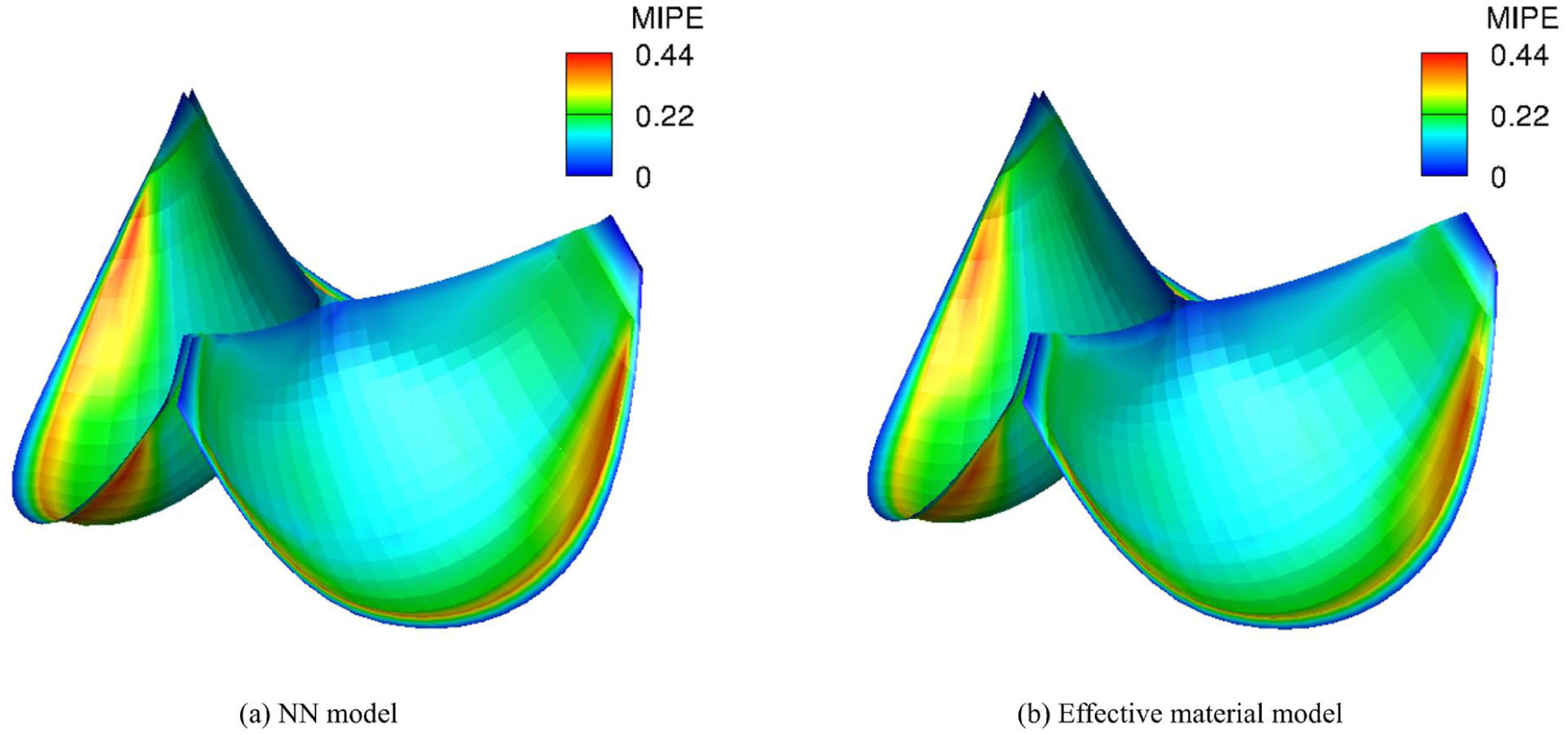
Verification of the simulation of tri-leaflet valves with the native porcine aortic valves properties using the NN model against an effective material model.

2.8. Numerical simulations conducted

The impact of the fiber structures to the strain distribution are further studied in a sequence of parametric simulations. Given different values of σ or different fiber directions (horizontal fiber and circumferentially aligned fibers (Fig. 12)), the strain distributions in the deformed state are obtained to demonstrate the impact of the fiber structures to the responses. Given the architectural trends in the normal and bicuspid aortic valves [20], we also exam the impacts of such population-based fiber structure to provide insights into mechanical factors affecting valvular function. A summary of fiber structures considered in the simulations is listed in Table 2. In all tri-leaflet simulations, the leaflet density and thickness are set to 1.0 g/cm³ and 0.0386 cm, respectively. The leaflet materials are crosslinked linked bovine pericardium. The tri-leaflet valves are loaded with an uniform pressure field of 80 mmHg to model the physiologic quasi-static transvalvular pressure at the closing stage. The penetration through the symmetric planes between the valve leaflets is penalized by a quadratic function of the penetration to simulate the contact between leaflets. The quasi-static solutions are approximated by dynamics simulations with mass damping to achieve steady states.

Fig. 12:

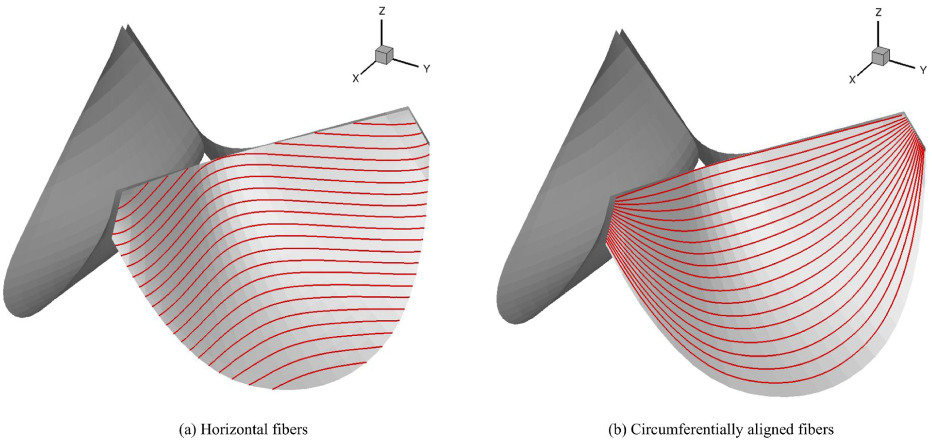
Two tri-leaflet heart valve models with different fiber directions (red lines).

Table 2:

Fiber structures for the numerical simulations conducted in the parametric studies.

θ	σ(ξ1, ξ2)
circumferential	32.66° everywhere
horizontal	32.66° everywhere
circumferential	mapped σ using BAV data
circumferential	mapped σ using TAV data
circumferential	10° everywhere
circumferential	20° everywhere
circumferential	30° everywhere
circumferential	50° everywhere

3. RESULTS

Effects of overall fiber directions.

The strain distributions with circumferentially and horizontally aligned fibers are shown in Fig. 13. The MIPE with horizontal fibers (Fig. 13a) is higher than the one with circumferentially aligned fibers (Fig. 13b). The maximum MIPE is slightly higher than 0.2. The fiber orientation on the heart valve significantly affects the strain fields. The overall MIPE distributions for both fiber directions have similar pattern. As shown in Fig. 13b and 13d, the MIPE for the circumferentially aligned fibers is close to the E_PD for most part except the region near the annulus. While the E_PD and E_XD for the horizontal fibers is very different especially on the belly and annulus. The effect of the fiber orientation to the strain is due to the high anisotropy of the material. The more anisotropic the material is, the more the effect of the fiber orientation.

Fig. 13:

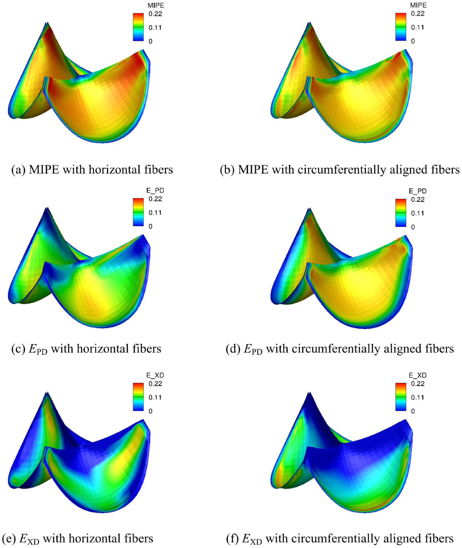
Strain distributions (MIPE, E_PD on the fiber direction, E_XD on the crossed in-plane direction) of the intact tri-leaflet valves with different fiber directions.

Effects of overall σs.

To demonstrate the effects of the dispersion of fiber splay σ we vary σ uniformly in the quasi-static simulations. The fibers are all circumferentially aligned. As σ increasing, the magnitude of E_PD is slowly increasing (Fig. 14) since less fibers are aligned circumferentially. This induces increasiong fibers dispersion so that more fibers are close to the cross directions. Thus, the magnitudes of E_XD on the belly region are significantly reducing (Fig. 15) as σ decreasing. Overall, the MIPE (Fig. 16) is gradually smoothed and achieves minimum average for σ = 30° among the four different σs due to the contribution of both E_PD and E_XD. This highlights the importance of the fiber structure mapping, showing how structural information impacts the overall deformation.

Fig. 14:

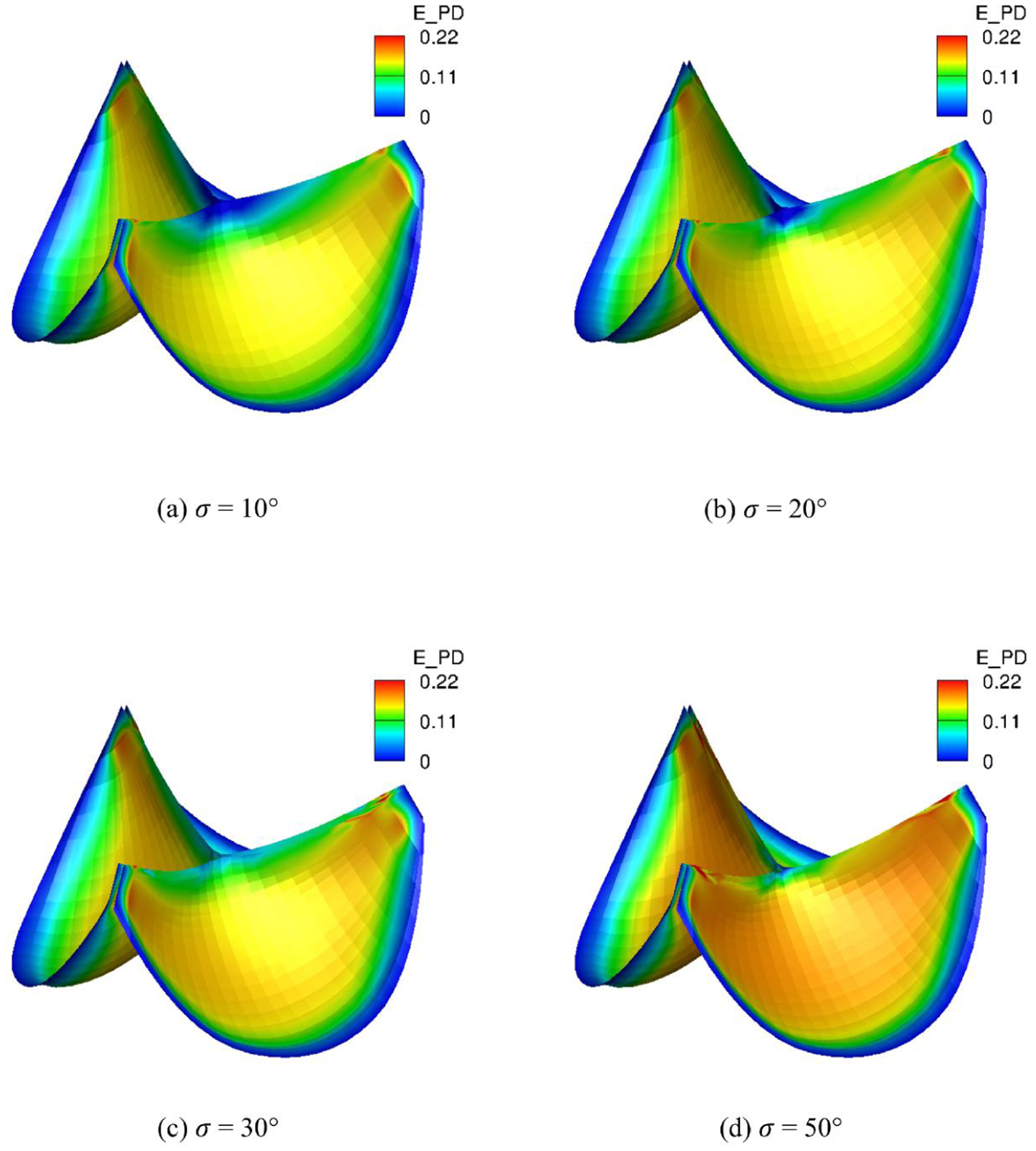
E_PD distribution of the intact tri-leaflet valves with σ = 10°, 20°, 30°, 50°.

Fig. 15:

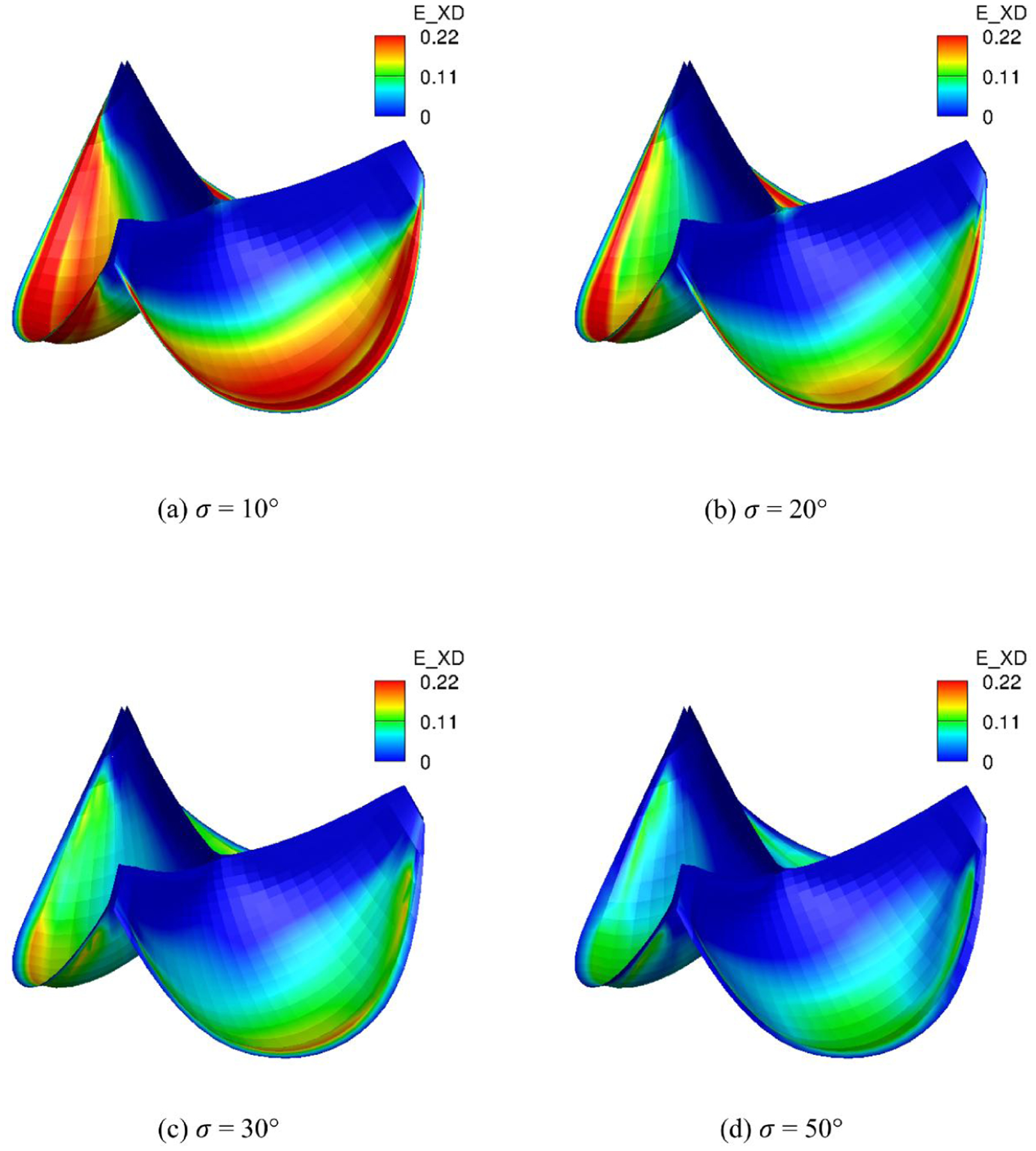
E_XD distribution of the intact tri-leaflet valves with σ = 10°, 20°, 30°, 50°.

Fig. 16:

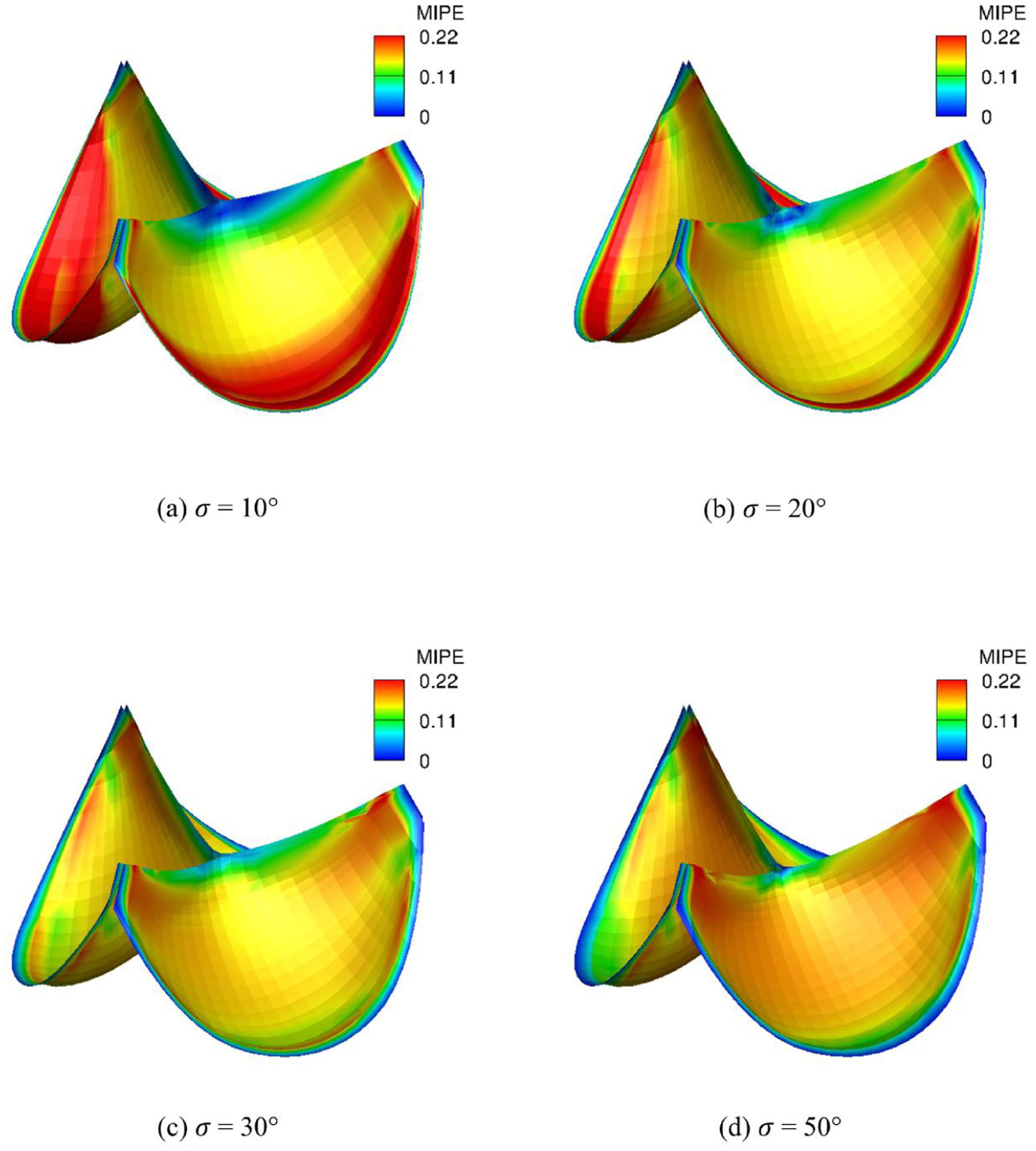
MIPE adistribution of the intact tri-leaflet valves with σ = 10°, 20°, 30°, 50°

Native AV and BAV fiber structures.

The NN model is integrated with the σ(ξ¹, ξ²) distribution for both BAV and TAV (Fig. 9) mapped on to each 3D valve leaflet. The NN model can predict the stresses at each material point with given local strains and σ(ξ¹, ξ²), and fiber directions using S(ξ¹, ξ²) = f_NN(E(ξ¹, ξ²), σ(ξ¹, ξ²)) − pC(ξ¹, ξ²)⁻¹. The strain distributions with σ mapping (Fig. 17) demonstrate significant differences from those with homogeneous distribution of σ especially for the strains in the preferred and cross directions (Fig. 14 and 15). Due to the heterogeneouty of the mapped fiber structures, fine-grained details emerge, which emphasizes the importance of the ability of NN models to predict the responses for a range of fiber structures. All three BAV strain fields (MIPE, E_PD, and E_XD) are overall higher and more heterogeneous than the TAV ones. The corresponding stress concentration may more likely leads to low heart valve durability.

Fig. 17:

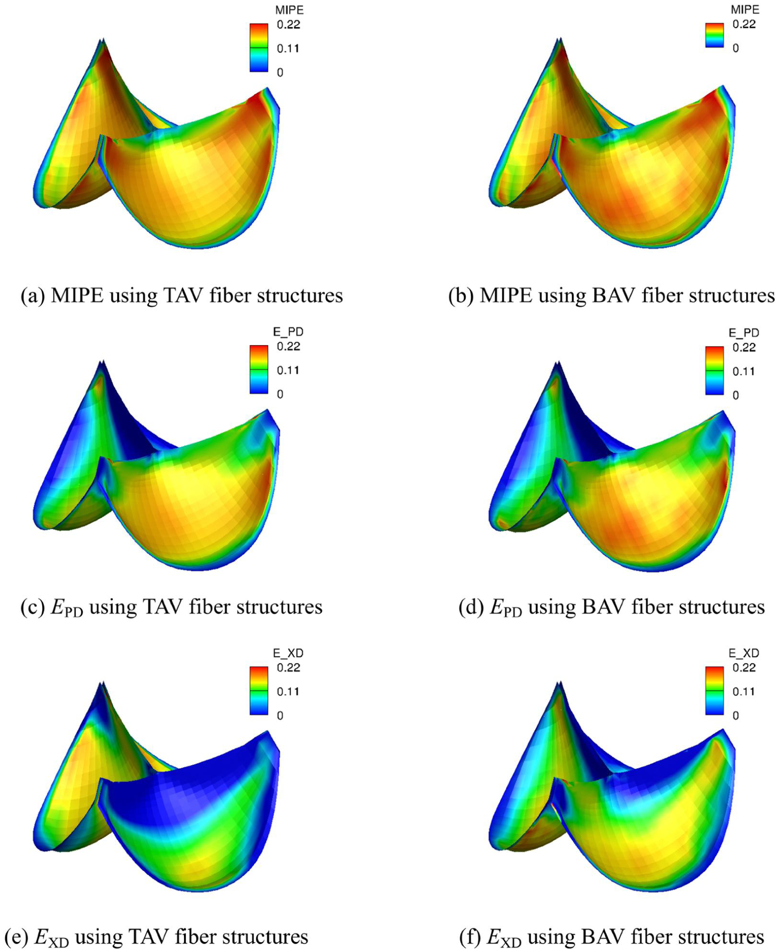
Strain distributions of the intact tri-leaflet valves using native bovine pericardium properties with σ mapping from BAV and TAV.

4. DISCUSSION

Overview.

In the present study, we developed an integrated tri-leaflet valve simulation pipeline built upon an IGA framework. A high-order structural tensor (HOST) based method was developed for efficient storage and mapping the fiber structure onto the valvular geometry. We then developed an artificial neural network (NN) material model that learned the responses of a detailed meso-structural model for both native and exogenously cross-linked heart valve leaflet tissues.

HOST representations of collagen fiber architectures.

Since the fiber orientation PDFs dictates the high anisotropy of the soft tissue mechanical responses, the AV simulations cannot give faithful clinical evaluation without mapped fiber structures. We have shown that with only 14 independent parameters the HOST representation can recover the ODFs of valvular tissues with negligible errors. The capability of the HOST method to facilitate the fiber structure mapping is further explored. A two-step procedure is established given the polar decomposition of the deformation tensor that represents the push forward from the excised flattened valvular tissue to the 3D in-vivo geometry. First, the stretched ODFs are obtained by the affine transformation of ODFs and the stretch tensor. Second, the HOST representations of stretched ODFs on the 3D surface are easily obtained by the standard tensor coordinate transformation using the rotation matrix. Finally, the deformed ODFs are recovered from the HOST representation. Thus, the HOST method is an efficient and robust representation of the ODFs that bridge that gap between the 2D fiber information obtained from the excised tissues and the 3D simulation models.

NN representations of material models.

The soft tissue material model needs to be not only informed by the fiber structure to give predictive capabilities but also efficient enough for trileaflet heart valve simulations performed in clinically relevant time-frames. The high-fidelity structural models and its extension for modeling long-term fatigue process [23] are based on the microstructural mechanism, however, it is in nature an ensemble model that involves double and quadruple integrals for native and crosslinked soft tissues. Even though the use of phenomenological models, such as the effective model we developed [24] can improve the computational efficiency significantly, it is not straight forward to extend such models to incorporate the structural parameters.

The NN material models were introduced to represent the stress-strain responses by training directly on the experimental data [29,27,25], which limits their predictability to prescribed protocols and specimens. While the present NN material models are trained on the responses generated by high-fidelity structural material models, which makes it predictable for the full range of physiological strains and structural parameters such as σ. Training on the responses generated by well-defined material models is also implicitly regulating the behavior of the NNs. As we examined in §2.4, even though symmetry and convexity constraints are not imposed in the training process, the violation of those constraints are not considerable.

Given the expressive power of the NNs, the use of NN material models presents a direct way to include the structural parameters that dictate the soft tissue responses. In this work, we trained a NN material model for crosslinked valvular material with a range of σ which dictates the anisotropy of the mechanical responses. The lower σ is, the more anisotropic the responses are. The trained NN material model is able to replicate the responses of the structural model for a range of σ, which demonstrates its expressive power for such applications. It not only fits the responses within the training range of strains with satisfactory relative errors but also captures trends of the responses two times more than the upper limit of the training stresses. This may be attributed to the unboundedness of softplus functions used as activation functions in the NN. The ability of capturing the response trends beyond the fitting range is useful for AV simulations when the resultant maximum strain is not known a prior. The use of the continuously differentiable softplus function also enables the NN material models to have continuous tangential stiffness matrices. This property is very important for the stability and convergence of AV simulations.

IGA implementation.

The NURBS geometry model for the fiber information storage and IGA simulations provides a modeling and analysis pipeline. The NURBS geometry can further streamline the iterating process of design and analysis. In this work, we explore the possibilities using NURBS to build an attributed-rich AV simulation model. It is enhanced with the population-based fiber structures for normal and bicuspid leaflets. The tIGAr library along with the FEniCS framework provides a unified framework for the IGA simulation with the NN material model. The analytical functions of the NN models represent are written in almost mathematical expressions in the Unified Form Language. The automatic differentiation of the FEniCS framework eliminates the need to manually derive the elasticity tensor and its implementation. With minimal modification of the present implementation, the NN material model is extensible to incorporate other structural parameters. The IGA formulation of K-L shell analysis provides C¹ solutions and smooth contact results. Although the AV models are equipped with NN material models, we show that it does not affect the computational speed significantly in comparison with the effective model. The simulation results with different σ distributions and fiber directions demonstrate the need to equip the AV simulation with realistic fiber information. The simulation results with the population-based fiber structures for normal and bicuspid leaflets show that the bicuspid leaflet have a more heterogeneous strain distribution and higher strains on the belly, which may ultimately reduce the durability of the leaflet in the long term.

Limitations.

For practical considerations, while the full Γ form was available, we only considered a simplified normal distribution, setup with the local coordinate system so that only one structural parameter σ was required. This allowed us to only require one structural parameter in the NN material model. It was clearly sufficient for demonstration of how a NN model trained complex structural model can produce highly flexible and accurate in-silico simulation results. That said, when greater fidelity of the Γ is required, the present NN model can be extended to include increasing numbers of the Fourier series components (up to 14). Most likely, for practical applications simplified forms (e.g. Gaussian Mixture models) can be developed to capture the level of mapped structural detail as needed. In any case, having a high fidelity local mapped structure will remain useful. The current UFL implementation of the NN models relied on the automatic differentiation to calculate the tangential stiffness matrix, which can be replaced by direct computation to reduce the computational overhead. This will also be needed for efficient implementation of IGA in FEniCS, wherein the UFL compilation adds to total compute time. Finally, we note too that there are alternative approaches for ODF mapping. For example, diffusion tensor imaging characterizes the diffusivity profile of tissue invivo by a single oriented 3D Gaussian probability distribution function. Methods to map ODFs include spherical harmonics and constructing a Riemannian space of the generalized ODFs, similar to that of traditional ODFs [58]. The present method retains advantages of both efficient storage and ease of mapping using tensor methods. That said, continued development of novel tissue imaging technologies will likely necessitate development of new mapping methods.

Future directions.

Regardless of the details of the design or delivery method all BHV exhibit limitations in durability, which continues to be in the range of 10–15 years. Moreover, these levels are often achieved only in patient ages 57 years or older [7]. BHV leaflet tissue failure results from leaflet structural deterioration mediated by fatigue and/or tissue mineralization [59,60]. These and other findings clearly demonstrate the need for an understanding the mechanisms of valve design/function and tissue degeneration to improve long-term durability.

To address these issues, the methods presented herein can assist in developing the next generation of replacement heart valves. Specifically while retaining the benefits of a high fidelity of the structural model, the present NN material models drastically reduced the computational cost. In comparison to the phenomenological models, regardless of specific form, the NN material model does not increase the computational cost for AV simulations. NN material models, as universal approximators, can be extended to represent more complex soft tissue mechanical behaviors, such as plasticity, fatigue, and related time-dependent behaviors [23]. Finally, with the advance of the in-vivo imaging techniques, the present AV model can be easily adapted to patient specific geometry and fiber structures when such data is available. In such circumstances, the predictability of the AV simulation will be significantly improved from a patient specific point of view.

5. APPENDICES

5.1. Implementation of the NN material model in FEniCS

The NN model can be easily embedded in the simulation with the help of the fiber structure mapping. The forward pass of NN model which gives the stress has an analytic and differentiable expression, f_NN(E, σ). The weight matrix W_l and bias vector b_l (l = 0, …, n_l) for the n_l-layer NN can be defined as constant matrix and vector. The element-wise softplus function can be defined as element-wise operator in the unified form language (UFL), which is part of the FEniCS project. A Python code snippet using UFL is shown in Listing 1. The FEniCS-based library can facilitate the resulting nonlinear variational problem solving by using the automatic differentiation capability. Thus, the overall simulation with NN models and fiber structure mapping can be conducted in the FEniCS framework.

Listing 1:

The Python code snippet for the NN material model

def E2S(E_PD, E_XD, E_phi, sigma, W0, b0, W1, b1, W2, b2):

″″″Compute the stress components using the NN material model.

Wi and bi (i = 0,1,2) are the weights and biases of the NN model.″″″

# An element–wise softplus function

def softplus (x, beta = 1., threshold = 20.):

def _elem_softplus (x, beta=beta, threshold=threshold):

return 1./beta*ln(exp(beta*x) + 1)

y = elem_op (_elem_softplus, x)

return y

# The NN model prediction

inputs = as_vector ([E_PD, E_XD, E_phi, sigma])

y1 = softplus (dot(W0, inputs) + b0)

y2 = softplus (dot(W1, y1) + b1)

outputs = dot (W2, y2) + b2

# Impose zero shear stresses for zero shear strains

multiplier = as_vector ([1., 1., E[2]])

S = elem_mult (multiplier, outputs)

return S

References

- 1.Schoen FJ, Current Opinion in Biotechnology 22(5), 698 (2011). DOI 10.1016/J.Copbio.2011.01.004. URL ://WOS:000296114600014 [DOI] [PubMed] [Google Scholar]
- 2.Schoen FJ, Levy RJ, Ann Thorac Surg 79(3), 1072 (2005). URL http://www.ncbi.nlm.nih.gov/entrez/query.fcgi?cmd=Retrieve&db=PubMed&dopt=Citation&list_uids=15734452 [DOI] [PubMed] [Google Scholar]
- 3.Schoen FJ, Cardiovasc Pathol 14(4), 189 (2005). URL http://www.ncbi.nlm.nih.gov/entrez/query.fcgi?cmd=Retrieve&db=PubMed&dopt=Citation&list_uids=16009317 [DOI] [PubMed] [Google Scholar]
- 4.Schoen FJ, Circulation 118(18), 1864 (2008). DOI 10.1161/CIRCULATIONAHA.108.805911. URL http://www.ncbi.nlm.nih.gov/entrez/query.fcgi?cmd=Retrieve&db=PubMed&dopt=Citation&list_uids=18955677 [DOI] [PubMed] [Google Scholar]
- 5.Cowell SJ, Newby DE, Prescott RJ, Bloomfield P, Reid J, Northridge DB, Boon NA, N Engl J Med 352(23), 2389 (2005). DOI 10.1056/NEJMoa043876. URL http://www.nejm.org/doi/pdf/10.1056/NEJMoa043876 [DOI] [PubMed] [Google Scholar]
- 6.Rajamannan NM, Current Treatment Options in Cardiovascular Medicine 7(6), 437 (2005). DOI 10.1007/s11936-005-0028-9 [DOI] [PubMed] [Google Scholar]
- 7.Kurtz CE, Otto CM, Medicine (Baltimore) 89(6), 349 (2010). DOI 10.1097/MD.0b013e3181fe5648 [DOI] [PubMed] [Google Scholar]
- 8.Yu PJ, Skolnick A, Ferrari G, Heretis K, Mignatti P, Pintucci G, Rosenzweig B, Diaz-Cartelle J, Kronzon I, Perk G, Pass HI, Galloway AC, Grossi EA, Grau JB, The Journal of Thoracic and Cardiovascular Surgery 138(1), 196 (2009). DOI 10.1016/j.jtcvs.2008.10.045 [DOI] [PubMed] [Google Scholar]
- 9.Parolari A, Tremoli E, Cavallotti L, Trezzi M, Kassem S, Loardi C, Veglia F, Ferrari G, Pacini D, Alamanni F, Heart 97(7), 523 (2011). DOI 10.1136/hrt.2010.215046. URL http://heart.bmj.com/content/97/7/523.full.pdf [DOI] [PubMed] [Google Scholar]
- 10.Siu SC, Silversides CK, J Am Coll Cardiol 55(25), 2789 (2010). DOI 10.1016/j.jacc.2009.12.068. URL http://www.ncbi.nlm.nih.gov/pubmed/20579534 [DOI] [PubMed] [Google Scholar]
- 11.Soares JS, Feaver KR, Zhang W, Kamensky D, Aggarwal A, Sacks MS, Cardiovascular Engineering and Technology 7(4), 309 (2016). DOI 10.1007/s13239-016-0276-8. URL 10.1007/s13239-016-0276-8 [DOI] [PMC free article] [PubMed] [Google Scholar]
- 12.Wu MCH, Zakerzadeh R, Kamensky D, Kiendl J, Sacks MS, Hsu MC, Journal of biomechanics 74, 23 (2018). DOI 10.1016/j.jbiomech.2018.04.012 [DOI] [PMC free article] [PubMed] [Google Scholar]
- 13.Hsu MC, Kamensky D, Xu F, Kiendl J, Wang C, Wu MCH, Mineroff J, Reali A, Bazilevs Y, Sacks MS, Computational mechanics 55, 1211 (2015). DOI 10.1007/s00466-015-1166-x [DOI] [PMC free article] [PubMed] [Google Scholar]
- 14.Votta E, Le TB, Stevanella M, Fusini L, Caiani EG, Redaelli A, Sotiropoulos F, J Biomech 46(2), 217 (2013) [DOI] [PMC free article] [PubMed] [Google Scholar]
- 15.Sturla F, Votta E, Stevanella M, Conti CA, Redaelli A, Medical Engineering and Physics 35, 1721 (2013) [DOI] [PubMed] [Google Scholar]
- 16.Aggarwal A, Sacks M, Lecture notes in Computer Science 9126, 285 (2015) [Google Scholar]
- 17.Aggarwal A, Sacks MS, Biomechanics and modeling in mechanobiology pp. 1–24 (2015)24718853 [Google Scholar]
- 18.Billiar KL, Sacks MS, J Biomech Eng 122(4), 327 (2000). URL http://www.ncbi.nlm.nih.gov/pubmed/11036555 [DOI] [PubMed] [Google Scholar]
- 19.Zhang W, Ayoub S, Liao J, Sacks MS, Acta Biomater 32, 238 (2016). DOI 10.1016/j.actbio.2015.12.001. URL http://www.ncbi.nlm.nih.gov/pubmed/26712602 [DOI] [PMC free article] [PubMed] [Google Scholar]
- 20.Aggarwal A, Ferrari G, Joyce E, Daniels MJ, Sainger R, Gorman JH 3rd, Gorman R, Sacks MS, Ann Biomed Eng 42(5), 986 (2014). DOI 10.1007/s10439-014-0973-0. URL http://www.ncbi.nlm.nih.gov/pubmed/24488233 [DOI] [PMC free article] [PubMed] [Google Scholar]
- 21.Goth W, Lesicko J, Sacks MS, Tunnell JW, Annual review of biomedical engineering 18, 357 (2016). DOI 10.1146/annurev-bioeng-071114-040625 [DOI] [PMC free article] [PubMed] [Google Scholar]
- 22.Goth W, Potter S, Allen ACB, Zoldan J, Sacks MS, Tunnell JW, Annals of biomedical engineering 47, 1250 (2019). DOI 10.1007/s10439-019-02233-0 [DOI] [PMC free article] [PubMed] [Google Scholar]
- 23.Zhang W, Sacks MS, Journal of the mechanical behavior of biomedical materials 75, 336 (2017). DOI 10.1016/j.jmbbm.2017.07.013 [DOI] [PMC free article] [PubMed] [Google Scholar]
- 24.Zhang W, Zakerzadeh R, Zhang W, Sacks MS, Journal of the mechanical behavior of biomedical materials 89, 168 (2019). DOI 10.1016/j.jmbbm.2018.09.016 [DOI] [PubMed] [Google Scholar]
- 25.Liang G, Chandrashekhara K, Engineering Structures 30(7), 2002 (2008). DOI 10.1016/j.engstruct.2007.12.021 [DOI] [Google Scholar]
- 26.Haj-Ali R, Kim HK, Mechanics of Materials 39(12), 1035 (2007). DOI 10.1016/j.mechmat.2007.05.004 [DOI] [Google Scholar]
- 27.Ghaboussi J, Sidarta D, Computers and Geotechnics 22(1), 29 (1998). DOI 10.1016/s0266-352x(97)00034-7 [DOI] [Google Scholar]
- 28.Hashash YMA, Jung S, Ghaboussi J, International Journal for Numerical Methods in Engineering 59(7), 989 (2004). DOI 10.1002/nme.905 [DOI] [Google Scholar]
- 29.Ghaboussi J, Pecknold DA, Zhang M, Haj-Ali RM, International Journal for Numerical Methods in Engineering 42(1), 105 (1998). DOI 10.1002/(SICI)1097-0207(19980515)42:1h105::AID-NME356i3.0.CO;2-V. URL https://onlinelibrary.wiley.com/doi/abs/10.1002/%28SICI%291097-0207%2819980515%2942%3A1%3C105%3A%3AAID-NME356%3E3.0.CO%3B2-V [DOI] [Google Scholar]
- 30.Thubrikar M, Piepgrass WC, Shaner TW, Nolan SP, Surg Forum 30, 241 (1979). URL http://www.ncbi.nlm.nih.gov/entrez/query.fcgi?cmd=Retrieve&db=PubMed&dopt=Citation&list_uids=538608 [PubMed] [Google Scholar]
- 31.Chandran KB, Kim SH, Han G, J Biomech 24(6), 385 (1991). URL http://www.ncbi.nlm.nih.gov/entrez/query.fcgi?cmd=Retrieve&db=PubMed&dopt=Citation&list_uids=1856239 [DOI] [PubMed] [Google Scholar]
- 32.Piegl L, Tiller W, The NURBS Book, 2nd edn. (Springer, 1997) [Google Scholar]
- 33.Kamensky D, Hsu MC, Schillinger D, Evans JA, Aggarwal A, Bazilevs Y, Sacks MS, Hughes TJ, Comput Methods Appl Mech Eng 284, 1005 (2015). DOI 10.1016/j.cma.2014.10.040. URL http://www.ncbi.nlm.nih.gov/pubmed/25541566 [DOI] [PMC free article] [PubMed] [Google Scholar]
- 34.Hsu MC, Kamensky D, Xu F, Kiendl J, Wang C, Wu MCH, Mineroff J, Reali A, Bazilevs Y, Sacks MS, Computational Mechanics pp. 1–15 (2015). URL 10.1007/s00466-015-1166-x [DOI] [PMC free article] [PubMed] [Google Scholar]
- 35.Kamensky D, Hsu MC, Schillinger D, Evans JA, Aggarwal A, Bazilevs Y, Sacks MS, Hughes TJR, A variational immersed boundary framework for fluid–structure interaction: Isogeometric implementation and application to bioprosthetic heart valves. Tech. rep (2014) [DOI] [PMC free article] [PubMed] [Google Scholar]
- 36.Hsu MC, Kamensky D, Bazilevs Y, Sacks MS, Hughes TJR, Computational Mechanics 54, 1055 (2014) [DOI] [PMC free article] [PubMed] [Google Scholar]
- 37.Sacks MS, Smith DB, Hiester ED, Journal of Biomedical Materials Research 41(1), 131 (1998) [DOI] [PubMed] [Google Scholar]
- 38.Logg A, Mardal KA, Wells G, Automated Solution of Differential Equations by the Finite Element Method the FEniCS Book, 2012th edn. Lecture Notes in Computational Science and Engineering, (Springer Berlin Heidelberg, Berlin, Heidelberg, 2012). URL http://UTXA.eblib.com/patron/FullRecord.aspx?p=885214 [Google Scholar]
- 39.Kassab GS, Sacks MS (eds.), Structure-Based Mechanics of Tissues and Organs (Springer; US, 2016). DOI 10.1007/978-1-4899-7630-7 [DOI] [Google Scholar]
- 40.May-Newman K, Yin FC, J Biomech Eng 120(1), 38 (1998). URL http://www.ncbi.nlm.nih.gov/htbin-post/Entrez/query?db=m&form=6&dopt=r&uid=0009675679 [DOI] [PubMed] [Google Scholar]
- 41.Sacks MS, Zhang W, Wognum S, Interface Focus 6(1), 20150090 (2016). DOI 10.1098/rsfs.2015.0090. URL http://rsfs.royalsocietypublishing.org/royfocus/6/1/20150090.full.pdf [DOI] [PMC free article] [PubMed] [Google Scholar]
- 42.Avazmohammadi R, Hill M, Simon M, Zhang W, Sacks M, Biomechanics and modeling in mechanobiology 16(2), 561 (2017) [DOI] [PMC free article] [PubMed] [Google Scholar]
- 43.Yang B, Lesicko J, Sharma M, Hill M, Sacks MS, Tunnell JW, Biomed. Opt. Express 6(4), 1520 (2015). DOI 10.1364/BOE.6.001520. URL http://www.osapublishing.org/boe/abstract.cfm?URI=boe-6-4-1520 [DOI] [PMC free article] [PubMed] [Google Scholar]
- 44.Smith DB, Sacks MS, Pattany PM, Schroeder R, J Heart Valve Dis 8(1), 25 (1999) [PubMed] [Google Scholar]
- 45.Amini R, Eckert CE, Koomalsingh K, McGarvey J, Minakawa M, Gorman JH, Gorman RC, Sacks MS, Ann Biomed Eng 40(7), 1455 (2012). DOI 10.1007/s10439-012-0524-5. URL http://www.ncbi.nlm.nih.gov/pubmed/22327292 [DOI] [PMC free article] [PubMed] [Google Scholar]
- 46.Aggarwal A, Pouch AM, Lai E, Lesicko J, Yushkevich PA, Gorman Iii JH, Gorman RC, Sacks MS, Journal of biomechanics 49, 2481 (2016). DOI 10.1016/j.jbiomech.2016.04.038 [DOI] [PMC free article] [PubMed] [Google Scholar]
- 47.Lee CH, Rabbah JP, Yoganathan AP, Gorman RC, Gorman JH 3rd, Sacks MS, Biomech Model Mechanobiol 14(6), 1281 (2015). DOI 10.1007/s10237-015-0674-0. URL http://www.ncbi.nlm.nih.gov/pubmed/25947879 [DOI] [PMC free article] [PubMed] [Google Scholar]
- 48.Lee CH, Zhang W, Liao J, Carruthers CA, Sacks JI, Sacks MS, Biophys J 108(8), 2074 (2015). DOI 10.1016/j.bpj.2015.03.019. URL http://www.ncbi.nlm.nih.gov/pubmed/25902446 [DOI] [PMC free article] [PubMed] [Google Scholar]
- 49.Kanatani KI, International Journal of Engineering Science 22(2) (1984) [Google Scholar]
- 50.Advani S, Tucker C III, Journal of Rheology 31(8), 751 (1987) [Google Scholar]
- 51.Fan R, Sacks MS, Journal of Biomechanics 47, 2043 (2014) [DOI] [PMC free article] [PubMed] [Google Scholar]
- 52.Teichert G, Natarajan A, der Ven AV, Garikipati K, Computer Methods in Applied Mechanics and Engineering 353, 201 (2019). DOI 10.1016/j.cma.2019.05.019 [DOI] [Google Scholar]
- 53.Lanir Y, Journal of Applied Mechanics-Transactions of the Asme 61(3), 695 (1994). URL ://A1994PJ70400029 [Google Scholar]
- 54.Xu F, Morganti S, Zakerzadeh R, Kamensky D, Auricchio F, Reali A, Hughes TJR, Sacks MS, Hsu MC, International journal for numerical methods in biomedical engineering (2017). DOI 10.1002/cnm.2938 [DOI] [PMC free article] [PubMed] [Google Scholar]
- 55.Sun W, Abad A, Sacks M, Journal of Biomechanial Engineering 127(6), 905 (2005) [DOI] [PubMed] [Google Scholar]
- 56.Zakerzadeh R, Hsu MC, Sacks MS, Expert review of medical devices 14, 849 (2017). DOI 10.1080/17434440.2017.1389274 [DOI] [PMC free article] [PubMed] [Google Scholar]
- 57.Kamensky D, Bazilevs Y, Computer Methods in Applied Mechanics and Engineering 344, 477 (2019). DOI 10.1016/j.cma.2018.10.002 [DOI] [PMC free article] [PubMed] [Google Scholar]
- 58.Du J, Goh A, Qiu A, in Biennial International Conference on Information Processing in Medical Imaging (Springer, 2011), pp. 448–462 [DOI] [PubMed] [Google Scholar]
- 59.Atkins SK, Cao K, Rajamannan NM, Sucosky P, Biomech Model Mechanobiol 13(6), 1209 (2014). DOI 10.1007/s10237-014-0567-7. URL http://www.ncbi.nlm.nih.gov/pubmed/24599392 [DOI] [PubMed] [Google Scholar]
- 60.Atkins SK, Sucosky P, World J Cardiol 6(12), 1227 (2014). DOI 10.4330/wjc.v6.i12.1227.URL http://www.ncbi.nlm.nih.gov/pubmed/25548612 [DOI] [PMC free article] [PubMed] [Google Scholar]