Deep Metric Learning for Cervical Image Classification

Abstract

Cervical cancer is caused by the persistent infection of certain types of the Human Papillomavirus (HPV) and is a leading cause of female mortality particularly in low and middle-income countries (LMIC). Visual inspection of the cervix with acetic acid (VIA) is a commonly used technique in cervical screening. While this technique is inexpensive, clinical assessment is highly subjective, and relatively poor reproducibility has been reported. A deep learning-based algorithm for automatic visual evaluation (AVE) of aceto-whitened cervical images was shown to be effective in detecting confirmed precancer (i.e. direct precursor to invasive cervical cancer). The images were selected from a large longitudinal study conducted by the National Cancer Institute in the Guanacaste province of Costa Rica. The training of AVE used annotation for cervix boundary, and the data scarcity challenge was dealt with manually optimized data augmentation. In contrast, we present a novel approach for cervical precancer detection using a deep metric learning-based (DML) framework which does not incorporate any effort for cervix boundary marking. The DML is an advanced learning strategy that can deal with data scarcity and bias training due to class imbalance data in a better way. Three different widely-used state-of-the-art DML techniques are evaluated- (a) Contrastive loss minimization, (b) N-pair embedding loss minimization, and, (c) Batch-hard loss minimization. Three popular Deep Convolutional Neural Networks (ResNet-50, MobileNet, NasNet) are configured for training with DML to produce class-separated (i.e. linearly separable) image feature descriptors. Finally, a K-Nearest Neighbor (KNN) classifier is trained with the extracted deep features. Both the feature quality and classification performance are quantitatively evaluated on the same data set as used in AVE. It shows that, unlike AVE, without using any data augmentation, the best model produced from our research improves specificity in disease detection without compromising sensitivity. The present research thus paves the way for new research directions for the related field.

I. INTRODUCTION

Cervical cancer is a major cause of premature female morbidity with over half a million new cases and over three hundred thousand deaths reported in 2018.¹ Universally, this disease is caused by persistent infection with one or more from a dozen oncogenic types of the human papillomavirus (HPV). Early detection of HPV-induced precancer (the precursor to cancer) and providing appropriate treatment where necessary can reduce suffering and premature death. However, there is a significant scarcity of clinical and gynecological services and expertise as well as a lack of sufficient access to effective low-cost cervical screening programs in the low and middle-income countries (LMIC). This shortage correlates highly with regions where the highest death rates have been reported.

The VIA method (Visual Inspection with Acetic Acid) is a low-cost and readily available screening method. A weak (3%-5%) acetic acid solution is applied to the cervix region which is then visually assessed by an expert. Whitening of cervical tissue around the transformation zone [1] indicates focal HPV infections. Appropriate treatment of the cervix or referral for further evaluation is recommended by the clinician. Although VIA is cheap and easily accessible, low reliability, accuracy, and high inter-observer variability have been reported [2]. Clinical colposcopes help in improving VIA performance with better illumination and optical magnification of the cervix region. However, they are very expensive and not commonly available in all settings. Moreover, these assessments also suffer from high intra- and inter-observer variability [3]. These challenges present an opportunity for research in developing powerful image analytics algorithms in an automated low-cost assistive screening system that is accurate, reliable, and effective.

There are several challenges towards achieving this goal. First, there is a lack of an imaging standard. We find that images are often taken inconsistently, with varied illumination, poor focus, high specular reflection, and imperfect color tone [4], [5]. Designing hand-crafted statistical features for addressing these variables is limiting and error-prone. Modern deep learning-based classification algorithms can apply data-driven strategies to deal with it in a better way. However, there is a naturally occurring high class-imbalance in screening data due to low disease prevalence in the general population with many more controls (normal class) than cases (abnormal class) -typical ratios of 99:1 or higher in controls to cases are not uncommon. This makes the tasks more challenging. Recall that, while DCNN is an important addition for representation learning in computer vision [6], [7], these networks are trained in an end-to-end manner, and during training adjust weight matrices within the network layers. Images are processed through the layers and produce prediction maps for all possible classes. The training error is computed based on the ground-truth probability map for every class, with a differentiable error function, such as Cross-Entropy, Mean Square Error, etc. However, key drawbacks of training a DCNN with classification loss are that it is prone to bias toward the majority class, which tends to be comprised of images from normal women. Such an imbalance does not guarantee, without an appropriate training strategy, that the image embedding (i.e. feature map obtained from the last fully connected layer before the loss layer) are linearly separable. While, it may sometimes appear that we obtain good classification accuracy, due to the classifier’s biasedness toward majority classes, we are often unable to get good feature representation to support generalization to unseen data.

Previously, Faster-RCNN, a deep learning-based Automatic Visual Evaluation (AVE) [8] method was proposed for detecting precancer cases. AVE uses a region proposal algorithm (Faster-RCNN) to localize the cervix boundary prior to the classification module. In developing AVE, the data skew was retained to increase statistical power for epidemiologic analyses but reduced to a 3:1 ratio of controls to cases. Consequently, in selecting absolute precancer cases the number of samples was also limited. With fewer data available for training, synthetic data augmentation was used during network training to overcome its impact on learning and classification performance. As a result, the trained model was likely over-fit to the data and less likely to adapt to naturally occurring variations in cervical image appearance and disease prevalence. In order to advance the prior AVE effort and pursue the first step toward addressing data skew, we develop a new method that operates on the full cervix image. We propose to train the convolutional neural network with deep metric learning (DML) for producing class-separated feature representation of the cervical images. Finally, a K-Nearest neighbor classifier is built with the deep features.

The key contributions of this paper are as follows.

1. We present a pioneering approach using deep metric learning for cervical precancer detection aimed at naturally occurring disease prevalence.

2. We analyze the linear separability of learned image features both quantitatively and qualitatively.

3. A detailed analysis of experimental results is conducted which demonstrates that the method improves specificity in disease detection without compromising sensitivity and paves the way for new research directions.

The organization of the rest of the paper is as follows: Section II provides background on state-of-the-art approaches on cervical image analysis. A discussion about deep metric learning and the experimented approaches are available in Section III. The experimental setup and the analysis of experimental results are presented in Section IV and Section V. Finally, Section VI concludes the paper.

II. RELATED LITERATURE

The potential for automatic analysis of digital cervical images in revolutionizing screening for precancers has motivated the development of several automatic and semi-automatic image analysis algorithms. These include algorithms for anatomical landmark detection [9], cervix region detection [10], [11], cervix type detection [12], pre-cancerous lesion detection-segmentation [13–15] and disease diagnosis [16–18]. Since our main concern is detecting precancer (or worst disease condition) in cervical images, we restrict our literature review to the topically relevant algorithms.

Early cervical image classification research mainly focused on the development of robust features to represent cervical images and classifier development. Commonly, hand-crafted image features were used as cervical image descriptors, such as (a) filter bank-based texture features, (b) pyramid color histogram features (in L*a*b* color space), (c) pyramid histogram of oriented gradients (PHOG), and (d) pyramid histogram of local binary patterns (PLBP). These features were subsequently used for developing classification algorithms, such as χ² distance, support vector machine (SVM), random forest (RF), gradient boosting decision tree (GBDT), AdaBoost, logistic regression (LR), multi-layer perceptron (MLP), and k-Nearest Neighbors (kNN) [16], [17], [19–21]. Some approaches extracted features from the cervix region-of-interest (RoI) detected at an earlier stage of the algorithm [16], [17]. However, these hand-crafted color and texture features were rarely sufficiently robust in representing cervical images due to high variability in image quality and appearance. The variability is most confounding in color and object illumination which are critical for disease discrimination, but also includes focus [4], the region of interest coverage, the imaging device, time that the image was taken after application of acetic acid, and geographic region [22]. This has resulted in data-driven automatic supervised representation learning algorithms becoming an attractive choice for computer vision researchers [8], [23–29]. Training a DCNN model from scratch was proposed in [23]. Multimodal learning [24], where image data along with clinical records are processed together has also been attempted. Multi-scale CNN are proposed in [25], [26]. Multi-CNN decision feature integration is used in [27]. [28] proposed to use the Deep Belief network. Object detection networks are employed in [8], [29].

All these approaches focus on developing a discriminating model, or classifier, from the raw color intensity matrix of the input images. In contrast, our research focuses on cervical image representation with deep metric learning.

III. METHODS

The deep metric learning (DML) is a robust technique that can address two limitations of commonly used deep classification networks- (i) biasedness towards majority class [30–32] and (ii) over-fitted model development due to data scarcity [33], [34]. The training strategy of DML aims to produce the image embedding in such a way that they are closer if the images are sampled from the same class and distant otherwise and thus produces class-separated image representation. Also, unlike classification model training, the training loss is computed based on the embedding obtained from multiple images. In the literature, several DML approaches are proposed which are broadly designed based on the image sampling strategy, embedding distance computation, loss computation etc. [30–32].

In this paper, we develop a DML based framework (see Fig 1 (a)) for cervical image classification. In the proposed framework, firstly, the DML is performed with the training images and their labels. The learning objective of DML is to produce a deep model which can generate class-discriminating feature vectors from the training images. Note that the deep network does not contain any classification layer during DML (see Fig 1(b)). In the next stage, the trained DML model serves as a feature extractor and extracted feature vectors are then used to build a K-Nearest Neighbor (KNN) classifier. During the test phase, the embeddings of the test images are obtained from the trained DML network and then their class labels are predicted from the trained KNN. We opt for a KNN classifier since the size of the training data is small and the features are expected to be linearly separable.

FIGURE 1.

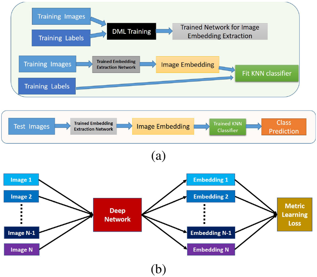
(a) Block diagram of the proposed system. Upper part denotes two-step training phase and lower part denotes test phase. (b) Block diagram of deep metric learning (DML). Images and their class labels are inputted and the mini-batch loss is computed based on the image embeddings.

In this paper, we vary learning objective functions (called loss functions) for deep model development with the DML. The loss functions associated with the chosen DML algorithms are described in the following paragraphs.

A. DEEP METRIC LEARNING WITH CONTRASTIVE LOSS

In this approach, a mini-batch is constructed with a randomly sampled pair of images. If the two images are sampled from the same class then the pair is called positive pair and if the images are sampled from different classes then the pair is called negative pair. The distance between a positive pair is called positive distance and the distance between a negative pair is called negative distance. The training loss is designed in a way such that the positive distance is minimized and the negative distance is maximized. Mathematically, the contrastive loss (L_contrastive) is defined as:

$$L_{contrastive}={\left[d_p-m_{pos}\right]}_{+}+{\left[m_{neg}-d_n\right]}_{+}$$ (1)

where m_pos denotes the upper limit of positive distance, m_neg denotes the lower limit of negative distance, d_p denotes positive distance, d_n denotes negative distance and ${\left[x\right]}_{+}=\max \left(0,\text{x}\right)$.

B. DEEP METRIC LEARNING WITH N-PAIR EMBEDDING LOSS

Suppose, X₁, Y₁, X₂, Y₂ …, X_N, Y_N are N-pair of images sampled from N different classes where X_i, Y_i are images from i^th class. The training loss between two i^th class images X_i and Y_i is given by

$$L_i=-\log \frac{\exp \left(f_{X_i}^T{f}_{Y_i}\right)}{{\sum }_{k=1,k\ne i}^N\exp \left(f_{X_i}^T{f}_{X_k}\right)+{\sum }_{k=1}^N\exp \left(f_{X_i}^T{f}_{Y_k}\right)}$$ (2)

where f_A is the feature vector of image A; and ^T representation transpose operation. The mini-batch loss is computed as the mean of all N classes, i.e., $L_{NPE}={\sum }_{i=1}^N{L}_i$. In the present work, N = 2 as we are dealing with binary classification problem.

C. DEEP METRIC LEARNING WITH BATCH HARD SAMPLING

In this approach, P classes² are randomly chosen and from every class, S images are randomly sampled. In a minibatch, the loss function considers the hard samples i.e. the maximum of intra-class (or positive) distances and minimum of inter-class (or negative) distances. The training loss is designed in a way such that it is decreasing the intra-class distance as well as increasing inter-class distance. Mathematically, the Batch-hard sampling loss (L_BH) is defined as:

$$L_{BH}={\sum _{i=1}^P\sum _{a=1}^S\left[m+\stackrel{\text{Intra-class distances}}{\overbrace{\underset{p=\mathrm{1..}S}{\min }D\left(f_a^i,f_p^i\right)}}-\stackrel{\text{Inter-class distances}}{\overbrace{\underset{\begin{array}{l}j=\mathrm{1..}P;n=\mathrm{1..}S\\ \text{ j}\ne \text{1}\end{array}}{\min }D\left(f_a^i,f_n^i\right)}}\right]}_{+}$$

where m is a predefined threshold, f denotes feature vector of an image, D(x, y) represents distance between x and y and ${\left[x\right]}_{+}=\max \left(0,\text{x}\right)$.

IV. EXPERIMENTAL SETUP

A. DATA SET DESCRIPTION

This paper uses Cervigram®³ image data set used in AVE research [8]. Every image in the data set was labeled either as a case (disease) or control (non-disease) based on the following diagnostic information: HPV status, naked-eye visual impression, colposcopic impression, cytological findings, histopathological analysis outcome. A sample image from both case and control class is shown in Fig 2.

FIGURE 2.

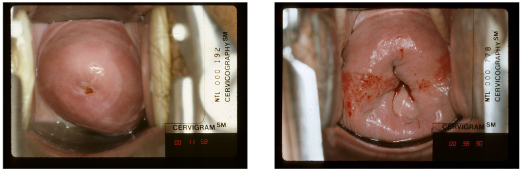
Samples of cervical images from the present data set. Left image from Control class. Right image from Case class.

In [8], the data set was partitioned into three nonoverlapping subsets: training, validation, and hold-out test sets, respectively. In our work, we make a random disjoint split of the training data into training and val1 data. The previous AVE validation data is termed val2. The val1 is used for parameter selection in the DML training. The val2 (i.e. validation data of [8]) is used for K value selection during classifier model building. The hold-out test data, which is the same as one used in AVE research, is used for comparing the classification performance with AVE. Details of data set splits are given in Table 1.

TABLE 1.

Age-stratified data set splits. The entries in the table denote the number of images.

Age-Group	Training		Val1		Val2		Hold-out Test
	Conrol	Case	Conrol	Case	Conrol	Case	Conrol	Case
<25	36	12	5	2	24	9	924	19
25-49	324	119	53	22	153	58	5010	45
>49	115	26	26	4	65	15	2232	20
Total	475	157	84	28	242	82	8174	85

B. DEEP NETWORKS AND TRAINING STRATEGIES

Three state-of-the-art pre-trained networks, namely, ResNet-50 [35], NasNetMobile [36] and Mobile-Net [37] are selected as backbone networks. First, the softmax classification layer is removed from each backbone network. Then an L2 normalization layer is used after the last feature layer of the networks. Finally, the networks are trained with the chosen DML algorithms (Section III). After training, the L2-normalized output vector obtained from the trained network is used as the image embedding. We vary the parameters associated with DML training best results are found when the DML are trained with learning rate = 0.002, weight decay = 1e – 6, and momentum = 0.9, epoch = 50. The DML algorithms built with constrictive loss and batch hard loss need to set loss function parameters. In this paper, we vary these parameters and receive best performance for following parameters (a) constrictive loss: m_pos = 0 and m_neg = 0.25, (b) batch hard loss: S = 8, m = 0.25.

C. BASELINE ALGORITHMS

The state-of-the-art pre-trained models developed using the ImageNet data are our initial choice as the baseline feature extractor networks. Note that the limitation of classification networks for imbalanced data set is our key concern. Our next baseline network is the fine-tuned binary classification network with our data. For this model development, we use binary cross-entropy loss minimization for training this classification network. The performance of the chosen DML algorithms is compared with these baselines.

D. PERFORMANCE EVALUATION

The proposed system has two steps: (1) Training deep model for linearly separable image embedding extraction, and (2) Classifier model development. We evaluate both steps separately. The evaluation scheme is described in the following subsections.

1). EMBEDDING QUALITY ASSESSMENT

We assess the quality of the feature embedding using t-SNE plots [38] visualization. The t-SNE converts the high dimensional data (here image embedding) into 2-D data vectors which help to visualize them in a 2D-plane. It is a very popular choice for data visualization in spite of its limitations. The t-SNE plot provides only a geometric interpretation of separation in the embedding at the cost of significant information loss in reducing high-dimensional data into a 2D vector. Moreover, small differences between feature vectors cannot be determined from the plot. To offset this limitation, we also propose using the following two quantitative measures for assessing embedding quality.

a: MEAN K-PRECISION

The K-precision of a test sample T is given by the ratio $\frac{k}{K}$, where k is the number of nearest neighbors of T of the same class selected among total K nearest neighbors from the training data. The mean K-precision is the mean of K-precision for all test images. The value of K-Precision lies in the range [0,1] and a higher value represents better performance.

b: CLASS-WISE MEAN N-PRECISION

Suppose, in the training data, there are N_control controls and N_case cases. The N-precision for a test data sample T_control belonging to the control class is given by the ratio $\frac{n_{control}}{N_{control}}$, where n_control is the number of nearest neighbors of T_control in the training set which belongs to control class. Similarly, N-precision for a test data sample T_case belonging to the case class is given by the ratio $\frac{n_{case}}{N_{case}}$, where n_case is the number of nearest neighbors of T_case in the training set which belongs to case class. The value of N-precision lies in range [0,1] and the higher value represent better performance. For a perfect model, all test data will have N-precision equals 1.

2). CLASSIFICATION PERFORMANCE EVALUATION

The classification performance is evaluated using class-wise accuracy. Class-wise accuracy is defined by the percentage of correct classifications achieved by the proposed model for each class. Note that the case accuracy refers to sensitivity/recall and the control accuracy refers to specificity. These two performance measures together can provide an idea about the biasedness of the model toward the majority class.

V. RESULTS AND DISCUSSION

The training loss and validation loss improvement for chosen DML algorithms are shown in Fig 3. According to Fig 3, the DML algorithm trained with Batch-hard loss has closer training and validation loss (val1) at the end of the training.

FIGURE 3.

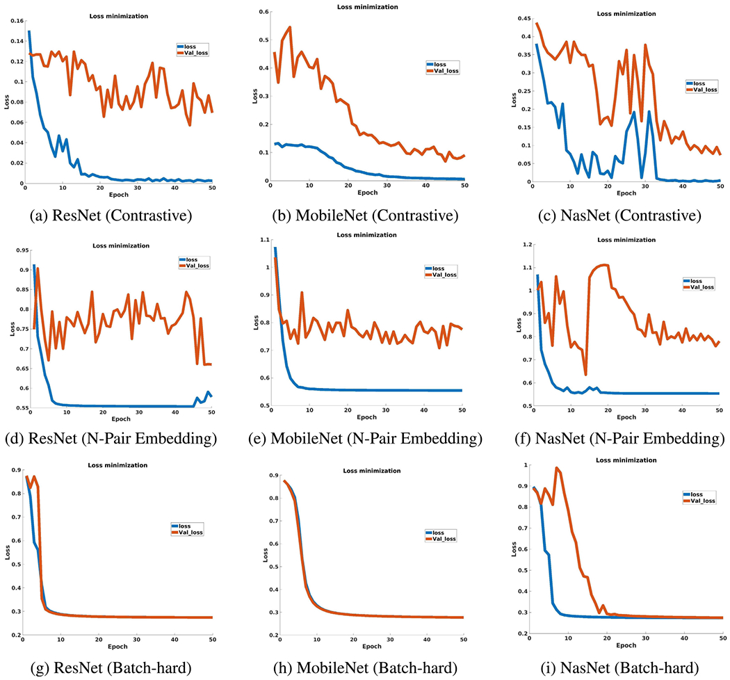
Loss improvement during DML training.

A detailed analysis of the experimental results is given in this section. We divide the discussion into four sections. The first section discusses the separability of the image embedding for the chosen algorithms. Next, we discuss the effectiveness of the K-Nearest Neighbour classifier. Then, the performance of the algorithm on the hold-out test data is presented. Finally, the performance of the best model is compared with the state-of-the-art AVE results [8].

A. EMBEDDING QUALITY ASSESSMENT

Fig 4 shows 2D t-SNE plots of the image embedding obtained from the considered competing approaches. In the first row, i.e., subfigures (a, b, c), show that the images are poorly separated when features from the ImageNet pre-trained networks are used. The second row, i.e., subfigures (d, e, f), shows that features from the fine-tuned models increase the separability. Finally, the last three rows, i.e., subfigures (g-o), demonstrate the power of DML which produces increasingly well-separated training image feature representations. We find that for many scenarios, due to the inability of producing fully generalized models with the chosen techniques, val2 images are not guaranteed to be closer to the appropriate class. However, based on our experiments, we can assert that the DML algorithm has the potential to deal with the current image classification task in a better way.

FIGURE 4.

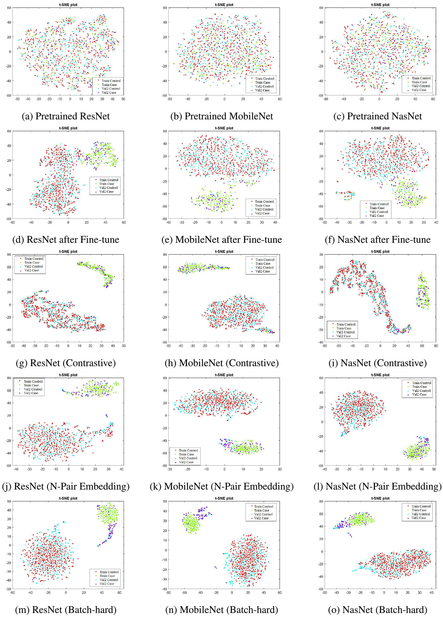
The t-SNE plots of feature embeddings.

The mean K-Precision for three different K values for all competing approaches for val2 data are given in Table 2. According to Table 2, the performance after fine-tuning with the training data is markedly improved over the pre-trained model. We also note that the performance of the deep networks built with contrastive loss based DML is comparable with the fine-tuned model. However, we see that the networks built with N-pair loss and Batch-hard sampling strategy outperform these competing methods.

TABLE 2.

Mean K-Precision in val2 data set. Network-wise best performing Mean K-Precision for different values of K are bold-faced.

Neighbour (K)	Network	Method
		Pre-trained	Fine-tuned	Contrastive	N-Pair Embedding	Batch-hard
1	ResNet-50	0.6512	0.9043	0.8920	0.9105	0.9198
	MobileNet	0.7099	0.9105	0.9074	0.9167	0.9105
	NasNet	0.6636	0.8704	0.9105	0.9228	0.9321
3	ResNet-50	0.6687	0.8992	0.8940	0.9115	0.9198
	MobileNet	0.6636	0.9043	0.8961	0.9167	0.9105
	NasNet	0.6605	0.8755	0.8961	0.9208	0.9321
5	ResNet-50	0.6784	0.8926	0.8932	0.9105	0.9198
	MobileNet	0.6611	0.9031	0.8951	0.9167	0.9105
	NasNet	0.6451	0.8716	0.8963	0.9204	0.9321

The mean N-Precision values of the case and control for all competing methods for val2 data are listed in Table 3. Here, we see that in terms of separability the embeddings obtained from the fine-tuned deep models are much better than the respective pre-trained models. The DML algorithms noticeably improve the mean N-Precision values for both cases and control over the fine-tuned models. Our experimental results also show that the networks trained with N-Pair embedding loss or Batch-hard loss minimization produce much better mean N-Precision values for cases than the networks trained with contrastive loss minimization. This demonstrates that the deep model developed with DML algorithm with Batch-hard or N-Pair Embedding loss minimization is valuable for producing separable image embedding for our classification task. We see this as a significant finding because real-world data are likely to be highly imbalanced with many more controls than cases. It is desirable to build classification models that adopt strategies built around this precondition thereby resulting in realistic and usable decisions.

TABLE 3.

Class-wise Mean N-Precision in val2 data set. The best performing feature representation method is chosen based on the average of Case and Control’s Mean N-precision. Network-wise best performing feature representation methods are bold-faced.

Network	Pre-trained		Fine-tuned		Contrastive		N-Pair Embedding		Batch-hard
	Control	Case	Control	Case	Control	Case	Control	Case	Control	Case
ResNet-50	0.7557	0.2458	0.8814	0.4273	0.9762	0.5593	0.9790	0.8119	0.9804	0.8361
MobileNet	0.7383	0.3305	0.8700	0.5027	0.9679	0.6385	0.9750	0.8725	0.9750	0.8482
NasNet	0.7381	0.3262	0.8766	0.5443	0.9714	0.6461	0.9709	0.8846	0.9696	0.9088

B. CLASSIFICATION PERFORMANCE

The class-wise K-Nearest Neighbor (KNN) classification accuracy for three different values of K in val2 data are shown in Table 4. Here, we see that the KNN classifiers trained with the pre-trained deep models are not suitable for our task. The performance of the DML algorithm trained with contrastive loss is comparable with fine-tuned models. For both approaches, keeping the network fixed results in good accuracy for controls but is found to be poor for cases. This is an indication of the classifier’s bias towards the majority class. Again, we see that for every network that was studied, the DML algorithm trained with N-pair embedding loss or Batch-hard loss is better at overcoming data imbalance and consequently the diminishing classifier bias. We surmise that the potential source of bias might be due to the model over-fitting to the training data. Finally, Table 4 shows that the NasNet model trained with Batch-hard loss minimization is our best deep model, and 1-NN (K = 1) can be considered as the best classifier because higher values of K increases the complexity and is unable to improve the classification performance.

TABLE 4.

KNN classification accuracy for val2 data set in percentage (%). The best performing classification model is chosen based on the average of Case and Control’s classification accuracy. The bold-faced numbers represent the network-wise best performing models for different values of K.

K	Network	Pre-trained		Fine-tuned		Contrastive		N-Pair Embedding		Batch-hard
		Control	Case	Control	Case	Control	Case	Control	Case	Control	Case
K=1	ResNet-50	78.93	24.39	95.45	75.61	96.28	68.29	94.63	76.83	94.63	84.15
	MobileNet	80.99	41.46	95.04	79.27	93.39	73.17	92.15	86.59	92.56	82.93
	NasNet	76.45	36.59	91.74	73.17	95.04	68.29	91.74	89.02	91.32	91.46
K=3	ResNet-50	88.43	18.29	96.28	73.17	96.69	68.29	95.87	80.49	94.63	84.15
	MobileNet	82.64	32.93	95.45	75.61	94.63	75.61	92.15	86.59	92.56	82.93
	NasNet	84.30	30.49	93.39	76.83	95.87	68.29	91.74	89.02	91.32	91.46
K=5	ResNet-50	95.04	10.98	95.04	71.95	96.69	68.29	94.21	80.49	94.63	84.15
	MobileNet	83.88	28.05	96.28	75.61	95.04	79.27	92.15	86.59	92.56	82.93
	NasNet	87.19	26.83	94.63	71.95	95.45	69.51	92.56	87.80	91.32	91.46

C. PERFORMANCE ON HOLD-OUT TEST SET

The mean K-Precision and class-wise mean N-Precision values for the hold-out test set are presented in Table 5 and Table 6, respectively. According to Table 5 all DML algorithms produce very good mean K-Precision for different values of K. As the hold-out test data is highly skewed (96:1) towards the control class and so mean K-Precision is not an effective measure as the good mean K-Precision may come from biased feature representation. Hence, we focus on Table 6 for performance comparison. According to Table 6, the mean N-Precision for control is good but the mean N-Precision for the case is not good for all networks. We see the balanced performance is obtained for the Batch-hard sampling approach and for NasNet it produces the best result.

TABLE 5.

Mean-K Precision on hold-out test set. Network-wise best results are bold-faced.

K	Network	Contrastive	N-Pair Embedding	Batch-hard
K=1	ResNet-50	0.9213	0.8964	0.8962
	MobileNet	0.8885	0.8918	0.8845
	NasNet	0.9139	0.8961	0.8514
K=3	ResNet-50	0.9274	0.8961	0.8962
	MobileNet	0.8877	0.8918	0.8845
	NasNet	0.9130	0.8959	0.8514
K=5	ResNet-50	0.9305	0.8959	0.8962
	MobileNet	0.8890	0.8918	0.8845
	NasNet	0.9118	0.8958	0.8514

TABLE 6.

N-Precision for hold-out test set. The best performing DML model is chosen based on the average of Case and Control’s mean N-precision. The network-wise best results are bold-faced.

Network	Contrastive		N-Pair Embedding		Batch-hard
	Control	Case	Control	Case	Control	Case
ResNet-50	0.9664	0.3951	0.9645	0.7014	0.9646	0.7365
MobileNet	0.9549	0.5061	0.9630	0.7365	0.9606	0.7598
NasNet	0.9575	0.5227	0.9643	0.7365	0.9495	0.8300

D. COMPARISON WITH THE STATE-OF-THE-ART

In [8], for the same data set, only the area under curve (AUC) values of the Receiver operating curve (ROC) were used to evaluate the classification model built with the Faster R-CNN algorithm. In this paper, for comparison purposes, we compute the age group-wise classification accuracies on the hold-out test set from the previous class prediction outcomes. Then the performance of the previous algorithm is compared with the best model produced from this research. According to the discussion presented in Section V-B, NasNet trained with Batch-hard loss minimization is our best feature extractor model and 1-NN is our best classifier. The age group-wise classification performance for our best model and the model built with the AVE algorithm is presented in Table 7. We see that the overall performance of our system outperforms the previously reported result. It is important to mention that we use the entire image and its class label. In contrast, the Faster R-CNN-based AVE algorithm uses additional annotation that localizes the cervix region of interest (ROI) during model training. We conclude that our method improves overall performance. We also compute the age-stratified Kappa statistics between our best model with previously reported Faster RCNN results, which are reported in Table 8.

TABLE 7.

Comparison with state-of-the-art on hold-out test data. This table shows overall and age-stratified (95% CI with exact binomial) comparison of best DML model with Faster RCNN [8]. Reported age stratified analysis excludes nine (9) women as their ages are missing.

Age Group	Method	Predicted Classes	Ground Truth
			Case	COL%	95% CI	Control	COL%	95% CI
All	Faster-RCNN	Case	71	83.5%	73.9% - 90.7%	1392	17.0%	16.2% - 17.9%
		Control	14	16.5%	9.3% - 26.1%	6782	83.0%	82.1% - 83.8%
	BH-NasNet-1-NN	Case	71	83.5%	73.9% - 90.7%	1213	14.8%	14.1% - 15.6%
		Control	14	16.5%	9.3% - 26.1%	6961	85.2%	84.4% - 85.9%
<25	Faster-RCNN	Case	15	78.9%	54.4% - 93.9%	212	22.9 %	20.3% - 25.8%
		Control	4	21.1%	6.1% - 45.6%	712	77.1%	74.2% - 79.7%
	BH-NasNet-1-NN	Case	14	73.7%	48.8% - 90.9%	220	23.8%	21.1% - 26.7%
		Control	5	26.3%	9.1% - 51.2%	704	76.2%	73.3% - 78.9%
25-49	Faster-RCNN	Case	43	95.6%	84.9% - 99.5%	800	16.0%	15.0% - 17.0%
		Control	2	4.4%	0.5% - 15.1%	4210	84.0%	83.0% - 85.0%
	BH-NasNet-1-NN	Case	41	91.1%	78.8% - 97.5%	692	13.8%	12.9% - 14.8%
		Control	4	8.9%	2.5% - 21.2%	4318	86.2%	85.2% - 87.1%
>50	Faster-RCNN	Case	12	60.0%	36.1% - 80.9%	380	17.0%	15.5% - 18.6%
		Control	8	40.0%	19.1% - 63.9%	1852	83.0%	81.4% - 84.5%
	BH-NasNet-1-NN	Case	15	75.0%	50.9% - 91.3%	301	13.5%	12.1% - 15.0%
		Control	5	25.0%	8.7% - 49.1%	1931	86.5%	85.0% - 87.9%

TABLE 8.

Confusion matrix of the best DML model (BH-NasNet-1-NN) and comparison with state-of-the-art performance on hold-out test data. This table shows overall and age stratified Kappa statistics between best DML model and Faster RCNN [8]. Reported age stratified analysis excludes nine (9) women as their ages are missing.

Age group	Faster RCNN	BH-NasNet-1-NN		Kappa
		Control	Case
All ages	Control	6613	183	0.76
	Case	362	1101
<25	Control	676	40	0.79
	Case	33	194
25-49	Control	4120	92	0.78
	Case	202	641
>50	Control	1809	51	0.70
	Case	127	265

VI. CONCLUSION

This paper takes a pioneering initiative to study the effectiveness of the deep metric learning algorithm for cervical image classification. Our experimental results show that the deep metric learning with Batch-hard loss minimization performs better than the previously proposed AVE method on the hold-out test set. Additionally, the present framework diminishes the image level ROI annotation labor. While our results are indeed better, we note that some misclassification still exists. The probable reason for this is the possible lack of proper generalizability during training. We believe that using more advanced metric learning techniques could overcome this deficit and is left for future work. The real-world application for the proposed system is to serve as an intelligent assistant for the clinician evaluating the woman. Also, the images used in the envisioned system could be acquired using a variety of devices, such as a smartphone, digital camera, or a colposcope enabled with digital image capture capability. These are likely to introduce additional image appearance variability, as noted earlier. Our future work shall also include steps to address this variability in addition to any data imbalance and regional variations in the appearance of the cervix.

Biographies

ANABIK PAL received the B.Sc. degree (Hons.) in computer science from the University of Calcutta, in 2008, the M.C.A. and M.E. degrees from Jadavpur University, in 2011 and 2013, respectively, and the Ph.D. degree in computer science from the Indian Statistical Institute, in 2019. He is currently a Postdoctoral Fellow with the Lister Hill National Center for Biomedical Communications (LHNCBC), U.S. National Library of Medicine (NLM), National Institutes of Health (NIH), Bethesda, MD, USA. His research interests include machine learning, data science, computer vision especially medical image analysis. He is a Life Member of the IUPRAI affiliated to IAPR.

ZHIYUN (JAYLENE) XUE received the B.S. and M.S. degrees from Tsinghua University, China, and the Ph.D. degree from Lehigh University, USA. Since 2006, she has been working with LHC on various medical imaging informatics projects. She is currently a Staff Scientist with the Lister Hill National Center for Biomedical Communications (LHC), National Library of Medicine (NLM). Her research interests include machine learning, computer vision, and medical image processing/analysis.

BRIAN BEFANO received the M.P.H. degree in epidemiology from the University of Massachusetts Amherst. He was previously with Information Management Services, Inc. He is currently pursuing the Ph.D. degree with the University of Washington. He has worked for over 15 years researching the natural history of HPV infections and their role in cervical carcinogenesis. He has been a technical consultant on multiple large-scale longitudinal cohort studies where he provided data management services and analytic support, with recent research focused on the application of artificial intelligence to cancer detection and screening.

ANA CECILIA RODRIGUEZ received the M.D. and Public Health degrees from the University of Costa Rica. She has dedicated the majority of her career to researching the natural history of cervical neoplasia and HPV infection and cervical cancer prevention strategies, including HPV vaccination, screening, and detection of cervical neoplasia. She has served as a Principal Investigator and a Co-Principal Investigator in Costa Rican studies funded by the National Cancer Institute, USA, including the Proyecto Epidemiologico Guanacaste (PEG) HPV Natural History Study, a 10,049 women longitudinal population-based cohort and the Costa Rican Vaccine Trial (CVT). She has dedicated her research to international efforts that will develop improved screening, triage and treatment methods more suitable for underserved and hard-to-reach populations.

L. RODNEY LONG received the B.A. and M.A. degrees in mathematics from The University of Texas, Austin, in 1971 and 1976, respectively, and the M.A. degree in applied mathematics from the University of Maryland, College Park, in 1987. He retired from the Communications Engineering Branch, National Library of Medicine, Bethesda, MD, USA, in 2020, where he has been as an Electronics Engineer, since 1990. He previously worked for 14 years in the industry as a Programmer and an Engineer. His research interests include content-based image retrieval, image processing, and image databases for biomedical applications.

MARK SCHIFFMAN received the M.D. degree from the University of Pennsylvania and the M.P.H. degree in epidemiology from the Johns Hopkins School of Hygiene and Public Health. He joined the National Cancer Institute, as a Staff Fellow, in 1983. He was appointed as the Chief of the Interdisciplinary Studies Section in the Environmental Epidemiology Branch (which later became the HPV Research Group in the Hormonal and Reproductive Epidemiology Branch), in 1996. He joined the Clinical Genetics Branch, in October 2009, to study intensively why HPV is such a powerful carcinogenic exposure, akin to an acquired genetic trait with high penetrance for a cancer phenotype. He has studied human papillomavirus (HPV) and cervical cancer for more than 35 years. He has conducted and collaborated on many large molecular epidemiologic observational studies and a few major trials through a natural progression of studies, he has pursued three main scientific themes, such as HPV Natural History and Cervical Carcinogenesis, Translational Studies of HPV Testing, Cytology, Colposcopy, and Vaccines, and Risk Prediction and Cervical Cancer Prevention. He received a Fulbright Scholarship, in 1977, to carry out epidemiologic studies in Senegal. He has received numerous awards for his work in molecular epidemiology, including the ACS Medal of Honor and the AACR Prevent Cancer Foundation Award.

SAMEER ANTANI (Senior Member, IEEE) received the Ph.D. degree in computer science and engineering from Pennsylvania State University. He is currently a Staff Scientist at the National Library of Medicine, part of the National Institutes of Health, leading research in machine learning and artificial intelligence (ML/AI) and biomedical image processing for automated clinical decisionmaking and analysis. He is a Senior Member of the International Society of Photonics and Optics (SPIE). He serves as the Vice-Chair for computational medicine on the IEEE Computer Society’s Technical Committee on Computational Life Sciences (TCCLS) and the Chair of IEEE Life Sciences Technical Community (LSTC). He is an Associate Editor for the MDPI journals Data and Diagnostics.

REFERENCES

- [1].Gaffikin L, Lauterbach M, and Blumenthal PD, “Performance of visual inspection with acetic acid for cervical cancer screening: A qualitative summary of evidence to date,” Obstetrical Gynecological Surv., vol. 58, no. 8, pp. 543–550, August. 2003. [DOI] [PubMed] [Google Scholar]
- [2].Jeronimo J, Massad LS, Castle PE, Wacholder S, and Schiffman M, “Interobserver agreement in the evaluation of digitized cervical images,” Obstetrics Gynecology, vol. 110, no. 4, pp. 833–840, October. 2007. [DOI] [PubMed] [Google Scholar]
- [3].Jeronimo J, Long LR, Neve L, Michael B, Antani S, and Schiffman M, “Digital tools for collecting data from cervigrams for research and training in colposcopy,” J. Lower Genital Tract Disease, vol. 10, no. 1, pp. 16–25, January. 2006. [DOI] [PubMed] [Google Scholar]
- [4].Guo P, Singh S, Xue Z, Long R, and Antani S, “Deep learning for assessing image focus for automated cervical cancer screening,” in Proc. IEEE EMBS Int. Conf. Biomed. Health Informat. (BHI), May 2019, pp. 1–4. [Google Scholar]
- [5].Guo P, Xue Z, Mtema Z, Yeates K, Ginsburg O, Demarco M, Long LR, Schiffman M, and Antani S, “Ensemble deep learning for cervix image selection toward improving reliability in automated cervical precancer screening,” Diagnostics, vol. 10, no. 7, p. 451, 2020. [DOI] [PMC free article] [PubMed] [Google Scholar]
- [6].LeCun Y, Boser B, Denker JS, Henderson D, Howard RE, Hubbard W, and Jackel LD, “Backpropagation applied to handwritten zip code recognition,” Neural Comput, vol. 1, no. 4, pp. 541–551, December. 1989. [Google Scholar]
- [7].Krizhevsky A, Sutskever I, and Hinton GE, “ImageNet classification with deep convolutional neural networks,” in Proc. Adv. Neural Inf. Process. Syst, Pereira F, Burges CJC, Bottou L, and Weinberger KQ, Eds. New York, NY, USA: Curran Associates, 2012, pp. 1097–1105. [Online]. Available: http://papers.nips.cc/paper/4824-imagenet-classification-with-deep-conv%olutional-neural-networks.pdf [Google Scholar]
- [8].Hu L, Bell D, Antani S, Xue Z, Yu K, Horning MP, Gachuhi N, Wilson B, Jaiswal MS, Befano B, Long LR, Herrero R, Einstein MH, Burk RD, Demarco M, Gage JC, Rodriguez AC, Wentzensen N, and Schiffman M, “An observational study of deep learning and automated evaluation of cervical images for cancer screening,” J. Nat. Cancer Inst, vol. 111, no. 9, pp. 923–932, September. 2019. [DOI] [PMC free article] [PubMed] [Google Scholar]
- [9].Greenspan H, Gordon S, Zimmerman G, Lotenberg S, Jeronimo J, Antani S, and Long R, “Automatic detection of anatomical landmarks in uterine cervix images,” IEEE Trans. Med. Imag, vol. 28, no. 3, pp. 454–468, March. 2009. [DOI] [PubMed] [Google Scholar]
- [10].Kanitkar A, Kulkarni R, Joshi V, Karwa Y, Gindi S, and Kale G, “Automatic detection of cervical region from VIA and VILI images using machine learning,” in Proc. IEEE Int. Conf. Comput. Sci. Eng. (CSE) IEEE Int. Conf. Embedded Ubiquitous Comput. (EUC), August. 2019, pp. 1–6. [Google Scholar]
- [11].Guo P, Xue Z, Long LR, and Antani S, “Cross-dataset evaluation of deep learning networks for uterine cervix segmentation,” Diagnostics, vol. 10, no. 1, p. 44, January. 2020. [DOI] [PMC free article] [PubMed] [Google Scholar]
- [12].Lei L, Xiong R, and Zhong H, Identifying Cervix Types Using Deep Convolutional Networks. Stanford, CA, USA: Stanford Univ. Report, 2017. [Google Scholar]
- [13].Alush A, Greenspan H, and Goldberger J, “Lesion detection and segmentation in uterine cervix images using an ARC-LEVEL MRF,” in Proc. IEEE Int. Symp. Biomed. Imag., From Nano Macro, June. 2009, pp. 474–477. [Google Scholar]
- [14].Alush A, Greenspan H, and Goldberger J, “Automated and interactive lesion detection and segmentation in uterine cervix images,” IEEE Trans. Med. Imag, vol. 29, no. 2, pp. 488–501, February. 2010. [DOI] [PubMed] [Google Scholar]
- [15].Meslouhi OE, Kardouchi M, Allali H, and Gadi T, “Semi-automatic cervical cancer segmentation using active contours without edges,” in Proc. 5th Int. Conf. Signal Image Technol. Internet Based Syst., November. 2009, pp. 54–58. [Google Scholar]
- [16].Srinivasan Y, Nutter B, Mitra S, Phillips B, and Sinzinger E, “Classification of cervix lesions using filter bank-based texture mode,” in Proc. 19th IEEE Symp. Comput.-Based Med. Syst. (CBMS), 2006, pp. 832–840. [Google Scholar]
- [17].Kim E and Huang X, A Data Driven Approach to Cervigram Image Analysis and Classification. Dordrecht, The Netherlands: Springer, 2013, pp. 1–13. [Google Scholar]
- [18].Fernandes K, Cardoso JS, and Fernandes J, “Automated methods for the decision support of cervical cancer screening using digital colposcopies,” IEEE Access, vol. 6, pp. 33910–33927, 2018. [Google Scholar]
- [19].Xu T, Xin C, Rodney Long L, Antani S, Xue Z, Kim E, and Huang X, “A new image data set and benchmark for cervical dysplasia classification evaluation,” in Machine Learning in Medical Imaging. Cham, Switzerland: Springer, 2015, pp. 26–35. [Google Scholar]
- [20].Xu T, Kim E, and Huang X, “Adjustable AdaBoost classifier and pyramid features for image-based cervical cancer diagnosis,” in Proc. IEEE 12th Int. Symp. Biomed. Imag. (ISBI), April. 2015, pp. 281–285. [Google Scholar]
- [21].Xu T, Zhang H, Xin C, Kim E, Long LR, Xue Z, Antani S, and Huang X, “Multi-feature based benchmark for cervical dysplasia classification evaluation,” Pattern Recognit., vol. 63, pp. 468–475, March. 2017. [Online]. Available: http://www.sciencedirect.com/science/article/pii/S0031320316302941 [DOI] [PMC free article] [PubMed] [Google Scholar]
- [22].Xue Z, Novetsky AP, Einstein MH, Marcus JZ, Befano B, Guo P, Demarco M, Wentzensen N, Long LR, Schiffman M, and Antani S, “A demonstration of automated visual evaluation of cervical images taken with a smartphone camera,” Int. J. Cancer, vol. 147, no. 9, pp. 2416–2423, November. 2020. [DOI] [PubMed] [Google Scholar]
- [23].Sato M, Horie K, Hara A, Miyamoto Y, Kurihara K, Tomio K, and Yokota H, “Application of deep learning to the classification of images from colposcopy,” Oncol. Lett, vol. 15, pp. 3518–3523, January. 2018. [DOI] [PMC free article] [PubMed] [Google Scholar]
- [24].Xu T, Zhang H, Huang X, Zhang S, and Metaxas DN, “Multimodal deep learning for cervical dysplasia diagnosis,” in Medical Image Computing and Computer-Assisted Intervention—MICCAI, Ourselin S, Joskowicz L, Sabuncu MR, Unal G, and Wells W, Eds. Cham, Switzerland: Springer, 2016, pp. 115–123. [Google Scholar]
- [25].Song N and Du Q, “Classification of cervical lesion images based on CNN and transfer learning,” in Proc. IEEE 9th Int. Conf. Electron. Inf. Emergency Commun. (ICEIEC), July. 2019, pp. 316–319. [Google Scholar]
- [26].Yue Z, Ding S, Zhao W, Wang H, Ma J, Zhang Y, and Zhang Y, “Automatic CIN grades prediction of sequential cervigram image using LSTM with multistate CNN features,” IEEEJ. Biomed. Health Informat, vol. 24, no. 3, pp. 844–854, March. 2020. [DOI] [PubMed] [Google Scholar]
- [27].Luo Y-M, Zhang T, Li P, Liu P-Z, Sun P, Dong B, and Ruan G, “MDFI: Multi-CNN decision feature integration for diagnosis of cervical precancerous lesions,” IEEE Access, vol. 8, pp. 29616–29626, 2020. [Google Scholar]
- [28].Rini Novitasari DC, Foeady AZ, Thohir M, Arifin AZ, Niam K, and Asyhar AH, “Automatic approach for cervical cancer detection based on deep belief network (DBN) using colposcopy data,” in Proc. Int. Conf. Artif. Intell. Inf. Commun. (ICAIIC), February. 2020, pp. 415–420. [Google Scholar]
- [29].Bai B, Du Y, Li P, and Lv Y, “Cervical lesion detection net,” in Proc. IEEE 13th Int. Conf. Anti-Counterfeiting, Secur., Identificat. (ASID), October. 2019, pp. 168–172. [Google Scholar]
- [30].Hadsell R, Chopra S, and LeCun Y, “Dimensionality reduction by learning an invariant mapping,” in Proc. IEEE Comput. Soc. Conf. Comput. Vis. Pattern Recognit. (CVPR), vol. 2, June. 2006, pp. 1735–1742. [Google Scholar]
- [31].Sohn K, “Improved deep metric learning with multi-class N-pair loss objective,” in Proc. Adv. Neural Inf. Process. Syst, Lee DD, Sugiyama M, Luxburg UV, Guyon I, and Garnett R, Eds. New York, NY, USA: Curran Associates, 2016, pp. 1857–1865. [Online]. Available: http://papers.nips.cc/paper/6200-improved-deep-metric-learning-with-mul%ti-class-n-pair-loss-objective.pdf [Google Scholar]
- [32].Hermans A, Beyer L, and Leibe B, “In defense of the triplet loss for person reidentification,” 2017, arXiv:1703.07737. [Online]. Available: https://arxiv.org/pdf/1703.07737.pdf [Google Scholar]
- [33].Chicco D, Siamese Neural Networks: An Overview. New York, NY: Springer, 2021, pp. 73–94, doi: 10.1007/978-1-0716-0826-5_3 [DOI] [PubMed] [Google Scholar]
- [34].Musgrave K, Belongie S, and Lim S-N, “A metric learning reality check,” in Computer Vision—ECCV, Vedaldi A, Bischof H, Brox T, and Frahm J-M, Eds. Cham, Switzerland: Springer, 2020, pp. 681–699. [Google Scholar]
- [35].He K, Zhang X, Ren S, and Sun J, “Deep residual learning for image recognition,” in Proc. IEEE Conf. Comput. Vis. Pattern Recognit. (CVPR), June. 2016, pp. 770–778. [Google Scholar]
- [36].Zoph B, Vasudevan V, Shlens J, and Le QV, “Learning transferable architectures for scalable image recognition,” in Proc. IEEE/CVF Conf. Comput. Vis. Pattern Recognit, June. 2018, pp. 8697–8710. [Google Scholar]
- [37].Howard AG, Zhu M, Chen B, Kalenichenko D, Wang W, Weyand T, Andreetto M, and Adam H, “MobileNets: Efficient convolutional neural networks for mobile vision applications,” 2017, arXiv:1704.04861. [Online]. Available: https://arxiv.org/pdf/1704.04861.pdf [Google Scholar]
- [38].Hinton G and Roweis S, “Stochastic neighbor embedding” in Proc. 15th Int. Conf. Neural Inf. Process. Syst. (NIPS), Cambridge, MA, USA: MIT Press, 2002, pp. 857–864. [Google Scholar]