

Abstract
We present a model and simulation for predicting the detected signal of a fluorescence-based optical biosensor built from optofluidic waveguides. Typical applications include flow experiments to determine pathogen concentrations in a biological sample after tagging relevant DNA or RNA sequences. An overview of the biosensor geometry and fabrication processes is presented. The basis for the predictive model is also outlined. The model is then compared to experimental results for three different biosensor designs. The model is shown to have similar signal statistics as physical tests, illustrating utility as a pre-fabrication design tool and as a predictor of detection sensitivity.
Keywords: Anti-resonant reflecting optical waveguides (ARROW), integrated waveguides, model design, optofluidics, predictive simulation
I. INTRODUCTION
OPTOFLUIDIC lab-on-a-chip devices for clinical diagnosis of pathogens tagged with fluorescing molecules are currently in commercial development [1]. These devices work by passing pathogen DNA or RNA, labeled with fluorescent markers, through hollow waveguides on a biosensor chip. Labeled particles flow past an optical excitation point and the resulting fluorescent light is coupled into a solid waveguide and guided off-chip to an avalanche photodetector. These biosensors have been used to detect viruses and bacteria, with some work spurred by a recent Ebola outbreak [2],[3] and the need to test for antibiotic resistant superbugs [1],[4]. Cancer biomarker detection is another possible application [5]. As with any optical sensor, achieving the highest possible sensitivity is important. For this particular biosensor, that requires getting as many fluorescent photons as possible to the photodetector.
These optofluidic biosensors rely on a complex microsystem that incorporates optics, waveguiding, fluid dynamics, and fluorescence. This paper outlines a comprehensive model that combines known models of physical behavior from each of these elements to predict the overall biosensor’s performance. Having such a model will allow us to predict the sensitivity of a particular biosensor design when changing parameters such as waveguide length and cross-section. Design geometries and material characteristics affect the optical signals generated and collected. Factors such as fluid flow speed and fluorescence behavior also influence the signal strength of a biosample. All these factors were built into the comprehensive model.
The paper will proceed as follows. We first briefly describe the fabrication process of a biosensor. Then we explain the theory of the prediction model and how the physics of the individual elements fit together. We then simulate three design variants. We compare experimental results of fabricated chips to simulation results from the model. Examining how closely the simulated and experimental results match, we show that the model can be used as a tool for the development of further biosensor designs. To make this comparison, we show simulated and measured optical peak signals for flow conditions. These data are presented in histogram plots binning expected signal strengths for a particle distribution, which have become our standard for reporting biosensor performance.
II. FABRICATION
Flow-through optofluidic biosensors are based on anti-resonant reflecting optical waveguides (ARROWs) [6],[7]. The devices are made by depositing periodic dielectric layers onto a blank silicon wafer. This series is three pairs of SiO2 and Ta2O5 with SiO2 deposited first. These layers are critical for guiding light in the liquid-core ARROW. The ARROW channel is formed by a layer of SU8, a negative photoresist. The resist is spun onto the wafer, baked, exposed, and developed. The result is a rectangular sacrificial structure, shown in Fig. 1a. Typical biosensors have a SU8 core 5-6 μm high, but a different design could call for a different height.
Fig. 1.

Overview of the biosensor fabrication process. (a) The SU8 sacrificial core is patterned and developed. (b) Pedestal is patterned and etched by DRIE. (c) A layer of silicon dioxide is grown over the pedestal and SU8 core. (d) The core of the ridge waveguide is etched into the silica layer by RIE. (e) A second silica layer of lower refractive index is grown as a cladding, (f) The sacrificial core is etched out to make the hollow channel.
A pedestal is etched by deep reactive ion etching (DRIE) for the waveguides, shown in Fig. 1b. Next, a layer of silicon dioxide (silica) is deposited by plasma-enhanced chemical vapor deposition (PECVD), as shown in Figure 1c. Typical designs require a 6-μm layer with a refractive index of 1.51. Next, we form a 4.5-μm tall ridge waveguide by RIE, though different designs may require different waveguide heights. The ridge is illustrated in Fig. 1d.
A low-index layer of silica, typically 6 μm with an index of 1.46, is deposited to protect the waveguides. This is shown in Fig. 1e. Finally, the SU8 sacrificial core is etched out with a sulfuric acid/hydrogen peroxide solution, leaving the ARROW channel open for a fluid solution to flow dining a biosensing operation. The final structure is shown in Fig. 1f.
III. THEORY AND MODEL CONSTRUCTION
Overview
Prior to introduction into the biosensor, a fluorescent marker solution is mixed with a processed biosample. The fluorescent markers will bond to a pathogen’s genetic material and can be identified by fluorescent light emitted by the markers. Some selected fluorophores also have quenched/unquenched feature, such that they will become unquenched and fluoresce only when bonded to a specific target.
The biosensor chip is built around a liquid-core ARROW as illustrated in Fig. 2. One prominent design uses an ARROW with an optically active segment 300-μm long and each end extending to a fluid reservoir. The 300-μm active segment couples with a ridge waveguide that collects fluorescence photons and guides them to the edge of the chip to a single-photon detector. Another ridge orthogonally intersects the ARROW’S 300-μm segment. This second ridge guides excitation light to the ARROW, creating an excitation region (ER) for fluorescent particles. These particles pass through the hollow ARROW, from one reservoir to the other. As the particles pass through the ER, fluorescent photons will generate and be collected by the collection ridge waveguide. These photons are the signal used for pathogen detection.
Fig. 2.

Overview diagram of biosensor chip. The fluorescent particles, bonded to pathogen targets will pass through the blue-shaded ARROW. An excitation mode is guided in a ridge waveguide that orthogonally intersects the ARROW. Fluorescence photons generated by the particles passing through the waveguide mode are collected into another ridge waveguide that couples with the ARROW, to be detected by an off-chip single-photon detector.
The excitation waveguide mode typically has a power profile that can be analyzed with a 2D Gaussian distribution, which extends across the width of the hollow ARROW channel, roughly illustrated by Fig. 3. This volume forms the ER, and the number of fluorescent photons a bioparticle emits depends on the x-y position of the bioparticle within the cross-section of the ARROW channel and the number of excitation photons incident on the bioparticle Passing through a more intense region of the waveguide mode, spending more time in the ER, and crossing through a more coupling-efficient part of the channel are all effects that will lead to a larger fluorescent signal delivered to an off-chip avalanche photodiode detector.
Fig. 3.

A close-up view of the excitation region in the biosensor. Fluorescent bioparticles flow through the active hollow core and pass through an excitation waveguide mode. Fluorescent light then guides down the length of the hollow core for detection.
An overview of the model construction process is given in Fig. 4, and a summary of model parameters used in this section’s figures are listed in {New Table I} at the end of the section.
Fig. 4.
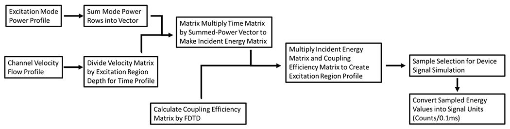
Overview of model consturction process. The final excitation region profile is created by the matrix multiplication of power and time factors to create a profile that represents the energy that would be incident on a particle passing through the excitation region. The incident energy is multiplied by a coupling efficiency matrix to create the excitation region profile. This matrix is then sampled to simulate a physical device’s behavior.
TABLE I.
Simulation Parameters for Example Model Construction
| Excitation Ridge Waveguide y/z Dimensions (μm) | 5 / 2 |
| Ridge Simulation Region y/z Mesh Grid | 25 / 25 |
| Input Laser Power (mW) | 3.0 |
| Excitation Waveguide Transmission | 2.2 |
| Channel x/y Dimensions (μm) | 12 / 5 |
| Channel x/y Mesh Grid | 60 / 25 |
| Mean Fluid Flow Velocity (cm/s) | 2.2 |
| Excitation Region Profile x/y Dimensions (μm) | 11.6 / 4.6 |
| Final Excitation Region Profile x/y Mesh Grid | 58 / 23 |
Fluorescent Marker Behavior
The maximum rate at which a fluorophore can emit a signal photon (Γm) is the inverse of its natural lifetime (τn) [8]. The natural lifetime can be found by dividing the fluorescence lifetime value (τ) by the quantum yield (Q). Using the ThermoFisher Scientific® Alexa Fluor 647 (AF647) as an example (Q = 0.33; τ = 1 ns) [9], the maximum fluorescent photon emission rate is 3.3×10⁸ s−1. The actual emission rate, however, is often limited by the incident exciting photon rate, as is the case in our system.
| (1) |
The rate that excitation photons are incident on a fluorophore (Γi) is the product of the photon flux (Φ) and the absorption cross section (σa) of the fluorophore. The flux is the power density, power divided by area (A), of the excitation source divided by the energy of an individual photon. In a typical setup, continuing the example of using AlexaFluor 647 as the signal soiuce, we use a 633-nm excitation laser (Plaser) set to 2-4 mW, but waveguide and facet transmission will reduce incident power in the ER. When the flux is multiplied against the fluorophore absorption cross section (1.03×10⁻¹⁵ cm2 for AF647) [10], [11], the typical photon incidence rate ranges from 6.1×l06 s−1 to 6.3×10⁷ s−1, depending on the excitation mode power and area. Since the incident photon rate is order(s) of magnitude lower than the maximum possible fluorescence photon emission rate, the effective fluorescence emission rate (Γe) is limited to the incident photon rate.
| (2) |
| (3) |
Waveguide Mode Profiles
By design, the excitation mode in the solid core waveguide has a 2D Gaussian-like profile, but depending on the excitation ridge geometry and index of refraction, the mode profile may have different areas or be divided between multiple mode lobes. This affects fluorescence generation as explained previously.
Using Lumerical® MODE Solutions mode simulations, we built a cross section of the excitation ridge waveguide that intersects the ARROW channel. Figure 5 gives example illustrations. A mesh size was chosen such that a single mesh cell approximated the size of the fluorescent particle under consideration. In the case of the experiments, further described later, we used a fluorescent bead with a 0.2 μm diameter; a rectangular mesh size of 0.2×0.2 μm2 was selected to contain a single simulated particle, as shown in Fig. 4a. An example of a very fine mesh, if called for in simulation, is shown in Fig. 4b.
Fig. 5.

Example Excitation Waveguide Mode Profile. Generated in Lumerical® MODE Solutions. (a) Mode profile with 0.2×0.2 μm2 mesh size. (b) Example of a profile with a very fine mesh size (1×1 nm2).
With this mesh, we simulated possible modes and selected those likely to occur in experimental tests. We exported the matrix of mode intensity values to MATLAB and normalized it by summing all the intensity (Im,o) values within the mode and dividing the matrix by that sum. We multiplied this normalized profile input laser power with the input laser power. Additionally, if the excitation ridge waveguide’s transmission (TWGex) is known, it can be multiplied against the normalized power profile. The power profile matrix (P) is defined as
| (4) |
The resulting matrix is a power profile, defined by y-z dimensions. The y-dimension corresponds with the mode height and ARROW channel height. The z-dimension corresponds with the mode width and ER depth in the channel. Since the waveguide profile is orthogonal to the ARROW channel, the fluorescent particles will flow across this laser profile. The bioparticles’ average velocity (0.88-2.25 cm/s) is great enough that in a laminar flow regime there is negligible deviation in their x-y positions while passing through the ER. Thus, we can assume that such deviation provides no error to the predictive model.
Under the assumption there is no x-y deviation in the particle’s path in the ER, the particle’s z-path is further assumed to be contained within a single row of the mode profile matrix. As the particle flows through the mode, it will be exposed to each mesh cell’s power value. To calculate the energy incident on the particle, we summed the power values in every row to create a single summed-power vector, illustrated in Fig. 6; this vector is one column wide and has an equal number of rows as the mode profile matrix. This summed-power vector will later be matrix multiplied with a time matrix to create an energy profile, explained below. This summed-power vector (Psum,m) is mathematically defined as
| (5) |
Fig. 6.

Example of a summed-power vector. The mode power profile is condensed to a single-column vector that contains the summed power values of every row.
Flow Velocity and Excitation Time Profiles
Based on a parabolic, laminar flow profile, fluid velocity in the channel varies with position, being fastest in the center and slowest at the sides and comers [12],[13]. When we define the depth of the ER in the direction of fluid flow, we divide the velocity of a given x-y position by the ER depth to determine the time a particle spends in the ER, absorbing light and fluorescing.
In MATLAB, we used a hilly developed fluid velocity model for a rectangular duct to create a velocity pro hie matrix (vi,j) for the ARROW channel [14]. An average flow velocity was chosen to match the velocity observed in experimental testing; the example model given in Fig. 7 was constructed with an average velocity of 2.2 cm/s. This average velocity changes based on both the channel cross sectional area and the applied pressiue in the channel inlet/outlet. The average velocity is typically 0.9-3.0 cm/s, and later sections will be more explicit in velocities used in simulations and physical experiments.
Fig. 7.

(a) Velocity profile of ARROW channel with an average velocity that can range from 0.8 to 3 cm/s. (b) Time spent in excitation region by x-y position in channel, defined as the depth of the excitation region divided by the flow velocity.
The sides of the duct were set to match the width and height of the channel. The number of rows was set to match the number of rows in the summed-power vector, and the number of columns was set to keep the same aspect ratio as the channel. At the above-stated velocities and in a laminar flow regime, we assumed a negligible x-y position deviation while the particle is in the ER. An example flow velocity profile matrix is illustrated in Fig. 7a.
To create the excitation time matrix (example given in Fig. 7b), we divided the depth of the ER (dER) by the velocity matrix calculated previously. The excitation region depth corresponds with the z-direction, and we defined it by the equating it with the exciting ridge waveguide width. The time profile matrix (ti,j) corresponds to the amount of time a fluorescent particle will spend in the excitation region based on its x-y position in the channel. The particle’s time in the ER can be defined mathematically as
| (6) |
Incident Energy and Coupling Efficiency Matrices
To determine the number of photons a particle in a given position within the channel will emit, we multiply the power a particle will absorb as it flows through the ER by the time in the region. The most fluorescence energy will be produced in an optimal x-y position that allows for intense excitation power and a slow velocity.
With the time matrix and a summed-power vector, we produced an incident excitation energy matrix (Einc;i,j) that calculates the amount of energy per area a fluorescent particle will receive based on the x-y position of the particle in the channel. The summed-power vector first was converted into a diagonal matrix of i×i size, with the vector’s values placed in the main diagonal of the new matrix. This summed-power diagonal matrix was then matrix-multiplied by the excitation time matrix. These processes can be defined as
| (7) |
| (8) |
| (9) |
When an element of this matrix is multiplied against the absorption cross section of a fluorophore, we calculate an energy amount that the fluorophore will absorb based on its position. This energy can be converted into a number of photons produced from a fluorophore passing through the ER. An example of the incident energy profile is given in Fig. 8.
Fig. 8.
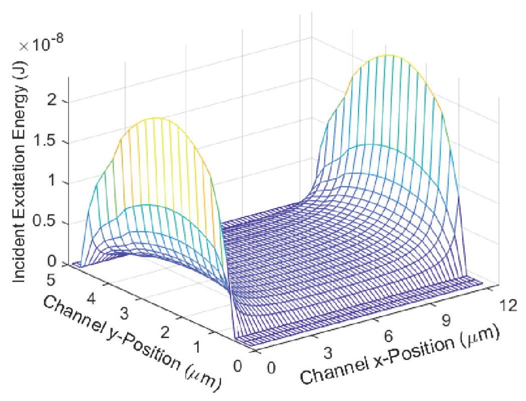
Incident excitation energy profile of ARROW channel.
It has also been observed that the percentage of generated fluorescence coupled into a mode in the ARROW channel depends on the fluorescent particle’s x-y position [15]. The coupling efficiency was found by a series of finite differential-time domain (FDTD) calculations [16]–[18]. We swept a dipole across the channel’s cross section and performed a FDTD simulation (using Lumerical® FDTD Solutions) at each sweep-point, measuring the power transmission value at a distance equal to the point the channel couples with the collection ridge waveguide. We performed this sweep with a dipole at various polarizations and at a wavelength equal to that of the fluorescence. We averaged the coupling efficiency matrices for each polarization to create an effective coupling efficiency profile (CEij). The coupling efficiency matrix was calculated to have the same dimensions as the incident excitation energy matrix so that a later Hadamard product may be found. Multiplying the energy matrix by the effective coupling efficiency matrix relates how many photons are coupled into a mode in the ARROW. Figure 9 illustrates an example profile of the ARROW’S coupling efficiency.
Fig. 9.

The FDTD-calculated coupling efficiency profile of the channel based on a fluorescent particle’s x-y position.
Final Excitation Region Profile and Simulating the Signal
After calculating the fluorescence production and coupling efficiency profiles, we get the form of the excitation region profile, with an example profile shown in Fig. 10a. Calculating the ER profile matrix (EER;i,j) is done by calculating the Hadamard product of the incident excitation energy and coupling efficiency matrices [19]. This calculation is shown as
| (10) |
Fig. 10.

(a) The model of the final excitation region profile is the product matrix of energy density and coupling efficiency matrices. This profile will change based on simulated optical mode, flow velocity profile, and ARROW cross-section dimensions. The outer rows and columns of values are removed as particles typically do not flow there in experimental findings. (b) Example simulated signal graph over chip run time. The signal magnitude is measured in “Counts/0.1ms”, the number of photons detected in a 0.1ms time bin. (c) Example distribution of signal magnitudes. The number of events (No. Events) is the number of particles detected within a signal bin.
In the case of excitation modes with a single lobe centered vertically in the channel’s y-direction, local peaks occur in the center of the channel where the peak intensity intersects with the peak coupling efficiency point. These local peaks can be lower than the peaks closer to the sidewalls of the channel due to the longer flow time on the sides. If the excitation mode is multi-lobed, the power will be divided between the lobes and will likely not intersect with the centered coupling efficiency peak. However, the lobes will intersect with a slower part of the channel and more photons may be emitted.
We next randomly selected a number of elements from the final energy matrix. This random selection is done with a uniform probability distribution, and the sampling was done with replacement to allow for particles to pass through the same position multiple times. Experimental results indicate that particles do not drag on the surface of the walls of the ARROW, but rather have a 0.2-0.5 μm minimum separation from the wall [20],[21]. Since the mesh cell size was 0.2 μm, we excluded from sampling the single rows and columns abutting the inner walls of the ARROW as defined in the model. This amounts to an exclusion of 10-16% of mesh cells from sampling; explicit sizes mesh dimensions of the ER profiles will be given below.
The selected energy values are converted into a number of photons incident on the particle. As the effective fluorescent photon generation rate is assumed to be the same as the incident photon rate, explained above, we approximate the photon signal count rate as the total number of photons generated by a fluorophore in a given position divided by the time spent in the ER. This conversion is done mathematically as
| (11) |
This photon count is then divided by time the respective particle is in the ER. This creates the signal as measured in counts/0.1ms, where 0.1 ms is the time bin set to approximate a passing particle’s time.
The model also assumes that only one event (a particle flowing through the ER) occurs at a time. For a given ER volume at a given instant and a test sample concentration of 107 particles/mL, there are approximately 3.6×10⁻³ events for every ER volume passed through the channel. For the purposes of this study, the frequency of double events is considered negligible.
We can simulate a signal measurement by placing the photon signal values on a time scale, as shown in Fig. 10b. For a given number of particles, we can find a mean signal (counts/0.1ms) and a distribution of signal magnitudes (Fig. 10c).
IV. SIMULATING THREE DESIGNS
To observe the biosensor’s design parameters’ effect on the expected signal, three designs were modeled and simulated for comparison. One is the standard biosensor geometry previously outlined and reported [22],[23]. Two newer designs are also studied, both with excitation ridge widths of 2 μm; the intention behind the reduced ridge width was to have a tighter, more intense excitation mode profile. The first new design is similar to the standard, but the heights of the ARROW core and ridge waveguide core are shortened. This design’s purpose was to increase the signal by having the mode field fill more of the channel’s height, leaving few low-intensity interactions. The second new design has an ARROW channel height of 5 μm, and the excitation waveguide is a rectangular high-index core centered on the ARROW height and completely “sandwiched” by low-index silica. The design here was to ensure a single-lobed mode would be centered on the peak of the coupling efficiency profile, increasing the maximum and mean signals.
These designs were fabricated, tested experimentally, and simulated. The avalanche photodiode used for photon counting was the Perkin Elmer® SPCM-AQR-14-FC, which has a stated efficiency of 65% [24]. For test fluorescent markers, we used ThermoFisher Scientific® FluoSpheres™ Carboxylate-Modified Microspheres. They were 0.2 μm in diameter and excited at a 633-nm wavelength. The sample we tested had a concentration of 107 beads/mL.
In the model and simulations, we used the solid waveguide transmissions that were found when characterizing the chips prior to bead flow-through testing. We chose to do this rather than simulate the waveguide losses as waveguide facet transmissions can vary based on the quality of the chip’s cleave from the silicon wafer. The test parameters for each device are listed in Table II.
TABLE II.
Design and Experiment Test Parameters
| Parameter | Standard | “Three-Micron“ | “Sandwich“ |
|---|---|---|---|
| Channel Dimensions [x by y] (μm) | 12×6 | 12×3 | 12×5 |
| Channel Mesh (Sampleable) [x by y] | 60×30 (58×28) | 60×15 (58×13) | 60×25 (58×23) |
| Excitation Region Depth (μm) | 5 | 2 | 2 |
| Laser Power (mW) | 3.9 | 3.6 | 3.3 |
| Ridge Waveguide Transmission | 0.15 | 0.43 | 0.38 |
| Average Flow Velocity (cm/s) | 0.90 | 0.88 | 2.25 |
| Sample Test Time (s) | 40 | 55 | 55 |
| Sample Test Volume (nL) | 56 | 29 | 75 |
| Number of Detected Beads | 512 | 443 | 1770 |
Standard Design
The most common (“standard”) design that has been used for these optofluidic biosensors consists of an ARROW core that is 6 μm high, and the excitation ridge is a 6-μm layer of 1.51-index silica and etched down 3.15 μm with a 5-μm width, illustrated in Fig. 11a. The mode profile in the standard design’s excitation ridge typically has one or two lobes in experimental tests, usually the result of coupling alignment by the excitation fiber; both cases are included in the simulations under study. The applied laser power was set to 3.9 mW, and the average flow velocity was 0.90 cm/s. Figures 11b and 11c show the respective excitation region profiles.
Fig. 11.

(a) Standard biosensor excitation ridge profile. (b) Excitation region profile of ARROW channel for a standard design with a double-lobe excitation mode. (c) Excitation region profile for a standard design with a single-lobe excitation mode.
One of the peaks of the double-lobed mode is not entirely contained within the ARROW channel, therefore some of the power from the laser does not reach the ER. Neither lobe intersects with the peak of the coupling efficiency profile, but both lobes do put most of their power in some of the slower regions of the flow velocity profile. By contrast, the single-lobe mode puts the power in the high-coupling efficiency and high-velocity portions of the ER. The simulation x-y mesh for the standard design was 60×30, and after the channel wall-adjacent mesh cells were excluded, the ER profile had a 58×28 mesh grid; 1624 cells were available for sampling. In the experiment, a sample volume of 56 nL was tested in a time of 40s (1.40 nL/s).
The signal from the two waveguide modes is similar, the main difference being the single-lobe mode has a higher maximum signal than the two-lobe mode. This is due to the mode being closely aligned with the peak of the y-component of the coupling efficiency profile. The difference in signal distributions is because the double-lobe mode has more counts in the lowest signal bin, and the single-lobe mode sees that bin reduced and higher-magnitude bins slightly increased.
Three-Micron Channel and Ridge
The fabrication process for the “Three-Micron” design is the same as the standard procedure except the ARROW channel has a height of 3 μm and the ridge waveguides are made of a silica layer 3 μm thick and etched down 2.25 μm, shown in Fig. 12a. The applied laser power was set to 3.6 mW, and the average flow velocity was 0.88 cm/s. The simulation x-y mesh for the “Three-Micron” design was 60×15, and after the channel wall-adjacent mesh cells were excluded, the ER profile had a 58×13 mesh grid; 754 cells were available for sampling.
Fig. 12.

(a) Geometry of “Three-Micron” excitation ridge waveguide. (b) Excitation region profile of ARROW channel for “Three-Micron” design.
The shorter channel height also restricts fluid flow through the channel, so a fluorescent particle will take a longer time to pass through the ER and produce more photons. A sample volume of 29 nL was tested in a time of 55 s (0.53 nL/s). The “Three-Micron” ER is shown in Fig. 12b. The intent of this design was to increase the mean signal by illuminating a greater proportion of the ER, and the simulation and experiment results will be explored below.
“Sandwich” Ridge Waveguide Design
The fabrication of the “Sandwich” waveguide follows the standard fabrication procedure except the silica layer for the ridge waveguide is a “sandwich” of three layers. The layers are 1 μm of low-index oxide, 3 μm of high-index oxide, and another 1 μm of low-index oxide. The ridge will be etched down by a minimum of 4 μm (past the interface between the bottom low-index oxide and the high-index oxide layers). When the chip is later covered by a low-index oxide layer, the effective waveguide is a rectangular high-index core completely surrounded by a low-index cladding, as shown in Fig. 13a. The applied laser power was set to 3.3 mW, and the average flow velocity was 2.25 cm/s. The simulation x-y mesh for the “Sandwich” design was 60×25, and after the channel wall-adjacent mesh cells were excluded, the ER profile had a 58×23 mesh grid; 1334 cells were available for sampling. In the experiment, a sample volume of 75 nL was tested in a time of 55 s (1.36 nL/s).
Fig. 13.

(top) Geometry of “sandwich” excitation waveguide. (bottom) Excitation region profile of an ARROW channel for a “sandwich” design.
The intended behavior of this design was to have a very tight and intense excitation mode that intersects the peak of the ARROW coupling efficiency profile. Figure 13b shows the predicted for the “Sandwich” design.
V. COMPARISON TO EXPERIMENTS
To compare the results given by the model and simulation to experimental results, the three biosensor designs were fabricated and tested with fluorescent microspheres flowing through the ER. The maximum, mean, and median signal statistics were found and compared between each simulation and its corresponding physical device.
To make this comparison between the model/simulation and the physical tests, some normalization was required. The first normalization requirement involves the magnitude of the detected signal. Because 0.2-μm diameter fluorescent beads were used and a quantified fluorescent equivalence between the beads and a single fluorescent marker was unknown (i.e. each bead is covered with many fluorophores and is brighter than a single fluorophore), a scalar multiplier was applied to the simulation to make the single-lobe standard simulation mean signal statistic roughly equivalent to the single-lobe standard physical test results. The scalar we found was 610, which would approximate to the number of illuminated fluorophores on one of the beads. This number was found by scaling up a multiplier on the randomly selected elements of the ER matrix for the standard device with a single-lobed excitation mode (Fig. 11c) until the simulated mean signal matched the respective experimental mean signal. This same scalar was then kept constant across all the designs’ simulations. As shown in Table I, using this common scalar produced intensity results between simulation and experiment that were quite comparable
A second normalization was required to keep equivalent the number of events in simulation and experiment. This was done by counting the total number of events registered in a physical test and simulating an equivalent number of beads, placed in random initial positions in the cross section of the fluid channel. This normalization effectively accounts for different bead concentrations from experiment to experiment and for different flow speeds within the channel. Using our two normalizations allows for direct comparison between the shape of the distribution curves between experiment and simulation and between the three designs in this study.
The signal distributions were also compiled and compared, along with standard deviation and coefficient of variance values. In a biosensor test, the desired output is a mean signal that is both high in intensity and as uniform as possible. The higher signal will make it more likely to detect a present target, and the greater uniformity will make that detection more reliable. The signal uniformity is measured by the standard deviation of signal peaks and their coefficient of variance (CV). As the standard deviation can increase with increasing mean signal, the coefficient of variance provides further information, defined as the standard deviation divided by the mean signal. Ideally, the standard deviations and coefficients of variance would be very small. Included in Table I are the 95% confidence ranges for the mean signals and standard deviations.
Additionally, the maximum signal and median signal statistics are included for comparison. The value of the maximum and median statistics, however, is limited to aiding an understanding of the respective histograms. The primary statistics used in evaluating a design’s behavior are the mean signal, standard deviation, and coefficient of variance. These statistics are shown in Table I.
The standard design had the smallest signal magnitudes in both the simulated model and physical tests. The maximum signal of the single-lobe simulation is significantly less than the found maximum of the “standard design” experiment, a 55.0% reduction; the simulated double-lobe maximum signal was 25.6% less than the experiment. The simulated single-lobe mean was used as the “anchor” for the fluorophore-per-bead scaling, so the matching values between simulation and experiment is to be expected. The double-lobe mean was 3.3% greater than the experiment. The standard design in experimental tests had a noise level of 3 counts/0.1ms and a signal-to-noise ratio (SNR) of 70.
The simulated mean signal of the “Three-Micron” design was 9.3% higher than the experiment. The maximum and median signals of the Three-Micron design were, respectively, 23.2% greater than and 36.6% greater than the experiment statistics. Critically, the mean signal of the “Three-Micron” design is approximately 4.0-4.2X greater than the standard design in simulation and 3.75X greater in physical experiment, making it the most sensitive of the three compared device designs. Physical tests also show a 18% smaller “Three-Micron” CV than the standard CV. The distributions of the “Three-Micron” signal (Fig. 14) reflect these improvements by having the mean extended furthest to the right than the standard. This distribution also appears to be the flattest of the three designs. The “Three-Micron design in experimental tests had a noise level of 11 counts/0.1ms and an SNR of 104, the highest SNR of the three studied designs.
Fig. 14.

Signal distribution comparisons of simulated and experimental signals. The signal magnitude is measured in “Counts/0.1ms”, the number of photons detected in a 0.1ms time bin; the number of events (No. Events) is the number of particles detected within a signal bin. (a) Standard design. (b) Three-Micron design. (c) “Sandwich” design.
The maximum signal of the simulated “Sandwich” design was 27.2% lower than the experimental maximum signal. The mean and median simulated signals were 3.0% greater and 16.2% greater, respectively, than the experiment statistics. The “Sandwich” mean signal is 2.3-2.4X greater than the standard in design in simulation and 2.3X greater than the standard mean signal in experiment. Physical experiments show an 18% smaller “Sandwich” CV than the standard CV and the smallest CV of all studied designs. The distributions of the “Sandwich” signal (Fig. 14) reflect these improvements by having the mean extended further out than the standard and a smaller spread relative to the mean. The “Sandwich” design in experimental tests had a noise level of 11 counts/0.1ms and an SNR of 73.
In each of the histogram distributions in Fig. 14, while each can be fitted with a normal distribution, the simulated distributions can still differ from their experimental counterparts. The simulated standard single lobe in Fig. 14a and the simulated “Three-Micron” in Fig. 14b are slightly more uniform than the respective experiments. The simulated “Sandwich” signal distribution in Fig. 14c has a few local peaks. Each ER profile will have its own distinctive effect on the distribution of sampled energy values, but these values are sampled with a uniform distribution with respect to x-y position. While no hydrodynamic focusing feature was intentionally included in these device designs, based on the discrepancies between simulation and experiment it can be conjectured that there is some particle x-y position preference for physical tests. There is no information at this time to comment further on this point. The model and simulation however do appear accurate enough to inform a future design’s signal performance.
The Three-Micron and “Sandwich” designs both show an increased mean signal over the older standard design. They both have higher standard deviations than the standard design partly due to the increased signal, but they have lower coefficients of variance than the standard, with the “Sandwich” CV being slightly lower than the Three-Micron’s. However, in a practical application, the mean signal (counts/0.1ms) is the primary statistic for measuring device performance and indeed pathogen detection. Simulation and experiment bear this out. The “Sandwich” has a faster fluid flow rate (1.36 nL/s) than the “Three-Micron” (0.53 nL/s) which would translate to a shorter test time in practice; in practical applications it may be the preferable option.
VI. DISCUSSION OF MODEL CAPABILITIES
The work presented here is a first attempt to model the behavior of the ARROW biosensor and to predict signal results based on design parameters. At the time of this paper’s writing, it does depend on the user selection of the excitation mode profile; this user selection will be influenced by prior knowledge of what mode is likely to occur in a physical device. Additionally, waveguide loss, facet transmission, and coupling transmission can vary based on defects in the fabrication process, quality of facet cleaves, and fiber alignment. Future development of the model should implement Monte Carlo simulations of the design parameter variabilities in a fabricated device. A model and simulation of noise levels in our devices would also be of interest for further development.
However, the model as presented here, when aided by known parameters, such as ridge waveguide transmissions and mode profiles, does present signal information that will assist the designer in planning a device fabrication process.
VII. CONCLUSION
Creating a model that can simulate an optofluidic biosensor’s performance required the integration of several areas of study. When microscopic waveguiding, microfluidic dynamics, and fluorescent behavior were properly integrated, we created a system that predicts the statistical behavior of a series of fluorescent particles passing through the excitation region. These predicted statistics are similar to physical test results and can inform the designer’s expectations of a device prior to device fabrication. Both the “Three-Micron” and “Sandwich” have an increased signal and improved signal uniformity compared to the standard design. The “Sandwich” design does not have quite the same signal magnitude as the “Three-Micron” design, but it is still an improvement on the signal from the standard design and has a shorter test time. Using the predictive model, we hypothesized the “Sandwich” design to be an improvement on the optofluidic biosensor technology and this was confirmed by experiment.
TABLE III.
Comparison of Simulated Signals and Physical Test Results
| Standard Design | “Three-Micron” Design | “Sandwich” Design | |||||
|---|---|---|---|---|---|---|---|
| Signal Statistic | Single Lobe Simulation* | Double Lobe Simulation | Physical Test | Simulation | Physical Test | Simulation | Physical Test |
| Maximum Signal (cts/0.1ms) | 796 | 1317 | 1769 | 4113 | 3339 | 2366 | 3252 |
| Mean Signal (cts/0.1ms) | 241 | 249 | 241 | 1251 | 1144 | 826 | 802 |
| Mean Signal - 95% Confidence Range (cts/0.1ms) | 228-254 | 232-266 | 227-255 | 1171-1331 | 1086-1202 | 804-847 | 783-824 |
| Median Signal (cts/0.1ms) | 231 | 203 | 209 | 1226 | 1070 | 817 | 703 |
| Standard Deviation (cts/0.1ms) | 150 | 192 | 161 | 855 | 626 | 458 | 413 |
| Standard Deviation - 95% Confidence Range (cts/0.1ms) | 142-160 | 182-205 | 152-172 | 802-915 | 588-670 | 434-474 | 400-427 |
| CV | 0.62 | 0.77 | 0.67 | 0.68 | 0.55 | 0.56 | 0.51 |
Simulation used to scale up the fluorophore-per-bead factor. This scalar was then kept constant across all other simulations.
Acknowledgment
The work shown here was financially aided by the funding of the National Institute of Health (NIH) under Grant No. 1R01AI116989 and 5R01EB028608.
Biographies
Joel. G. Wright, Jr. (S’15) received the B.S.E. degree in electrical engineering from Arizona State University, Tempe, AZ, USA in 2015. He is a Ph.D. candidate at Brigham Young University in the Electrical and Computer Engineering Department. His current research includes the fabrication of optics-based biosensors and computer modeling such devices.
Md Nafiz Amin obtained his B.Sc. degree in Electrical & Electronic Engineering from Bangladesh University of Engineering & Technology (BUET), Bangladesh in 2015. Currently he is a PhD student in the ECE department, University of California, Santa Cruz. His present research interest includes design and optimization of integrated photonic sensors for different applications.
Gopikrishnan Gopalakrishnan Meena received his Integrated Masters in Science degree in physics from University of Hyderabad, Hyderabad, Andra Pradesh, India in 2013. He is currently working towards the Ph.D degree in electrical and computer engineering at the University of California, Santa Cruz. His research interest includes integrated photonic devices and optofluidic devices for biosensing and diagnostic applications. He has been a member of Applied Optics group at University of California Santa Cruz since 2014. He is the recipient of a first-year QB3 Fellowship through the W.M. Keck Center for Nanoscale Optofluidics.
Holger Schmidt (F’17) received his Ph.D. in electrical and computer engineering from the University of California, Santa Barbara. He served as a postdoctoral fellow with MIT. Currently, he is the Narinder Kapany Chair of optoelectronics, a professor of electrical and computer engineering and the associate dean for research with the Baskin School of Engineering, University of California, Santa Cruz. His research interests include integrated photonics, optofluidics, single molecule analysis, nanomagnetism, and spintronic devices. He has authored or coauthored over 400 publications and is a Fellow of the OSA, IEEE, and NAI.
Aaron R. Hawkins (F’16) received a B.S. degree from Caltech and a Ph.D. degree from the University of California, Santa Barbara. He was a Co-founder of Terabit Technology and an engineer at CIENA and Intel. He is currently a Professor with the Electrical and Computer Engineering Department, Brigham Young University, doing research in optofluidics, integrated optics, and MEMs. He has authored or coauthored over 400 technical publications and is a Fellow of the IEEE and the OSA. He has served as the Editor-in-Chief for the IEEE Journal of Quantum Electronics and currently serves as the IEEE Photonic Society’s VP of Publication.
Footnotes
Disclosures
A.R.H. and H.S. have a financial interest in Fluxus Inc., which commercializes optofluidic technology.
Contributor Information
Joel G. Wright, Jr, Department of Electrical and Computer Engineering, Brigham Young University, Provo, UT, 84602, USA.
Md Nafiz Amin, School of Engineering, University of California Santa Cruz, Santa Cruz, CA 95064, USA.
Gopikrishnan G. Meena, School of Engineering, University of California Santa Cruz, Santa Cruz, CA 95064, USA
Holger Schmidt, School of Engineering, University of California Santa Cruz, Santa Cruz, CA 95064, USA.
Aaron R. Hawkins, Department of Electrical and Computer Engineering, Brigham Young University, Provo, UT, 84602, USA.
References
- [1].Meena GG, Hanson RL, Wood RL, Brown OT, Stott MA, Robison RA, Pitt WG, Woolley AT, Hawkins AR, and Schmidt H, “3X multiplexed detection of antibiotic resistant plasmids with single molecule sensitivity”, Lab Chip, vol. 20, pp. 3763–3771, Sept. 2020, doi: 10.1039/D0LC00640H. [DOI] [PMC free article] [PubMed] [Google Scholar]
- [2].Du K, Cai H, Wall TA, Stott MA, Alfson KJ, Griffiths A, Carrion R, Patterson JL, Hawkins AR, Schmidt H, and Mathies RA, “Multiplexed Efficient On-Chip Sample Preparation and Sensitive Amplification-Free Detection of Ebola Virus”, Biosens. Bioelectron, vol. 91, pp. 489–496, January. 2017, doi: 10.1016/j.bios.2016.12.071. [DOI] [PMC free article] [PubMed] [Google Scholar]
- [3].Cai H, parks JW, Wall TA, Stott MA, Stambaugh A, Alfson K, Griffiths A, Mathies RA, Carrion R, Patterson JL, Hawkins AR, and Schmidt H, “Optofluidic Analysis System for Amplification-free, Direct Detection of Ebola Infection”, Sci. Rep, vol. 5, Art. no. 14494, September. 2015. [DOI] [PMC free article] [PubMed] [Google Scholar]
- [4].Meena GG, Wall TA, Stott MA, Brown O, Robison R, Hawkins AR, and Schmidt H, “7X multiplexed, optofluidic detection of nucleic acids for antibiotic-resistance bacterial screening”, Opt. Express, vol. 28, no. 22, pp. 33019–33027, 2020, doi: 10.1364/OE.402311 [DOI] [PMC free article] [PubMed] [Google Scholar]
- [5].Cai H, Stott MA, Ozcelik D, Parks JW, Hawkins AR, and Schmidt H, “On-chip wavelength multiplexed detection of cancer DNA biomarkers in blood”, Biomicrofluidics, vol. 10, no. 6, Art. no. 064116, Dec. 2016, doi: 10.1063/1.4968033. [DOI] [PMC free article] [PubMed] [Google Scholar]
- [6].Duguay MA, Kokubun Y, Koch T, and Pfeiffer L, “Antiresonant reflecting optical waveguides in SiO2-Si multilayer structures,” Appl. Phys. Lett, vol. 49, no. 13, pp. 13–15, May 1986, doi: 10.1063/1.97085. [DOI] [Google Scholar]
- [7].Yin D, Schmidt H, Barber JP, and Hawkins AR, “Integrated ARROW waveguides with hollow cores,” Opt. Express, vol. 12, no. 12, pp. 2710–2715, June 2004, doi: 10.1364/OPEX.12.002710. [DOI] [PubMed] [Google Scholar]
- [8].Lakowicz JR, “Introduction to Fluorescence”, in Principles of Fluorescence Spectroscopy, 3rd ed., New York: Springer, 2006, ch. 1, pp. 9–10. [Google Scholar]
- [9].ThermoFisher.com. “Fluorescence Quantum Yields (QY) and Lifetimes (τ) for Alexa Fluor Dyes – Table 1.5.” https://www.thermofisher.com/us/en/home/references/molecular-probes-the-handbook/tables/fluorescence-quantum-yields-and-lifetimes-for-alexa-fluor-dyes.html (accessed October 20, 2020).
- [10].Lakowicz JR, “Instrumentation for Fluorescence Spectroscopy”, in Principles of Fluorescence Spectroscopy, 3rd ed., New York: Springer, 2006, ch. 2, p. 59. [Google Scholar]
- [11].ThermoFisher.com “The Alexa Fluor Dye Series—Note 1.1.” https://www.thermofisher.com/us/en/home/references/molecular-probes-the-handbook/technical-notes-and-product-highlights/the-alexa-fluor-dye-series.html (accessed October 20, 2020).
- [12].Shah RK and London AL, “Rectangular Ducts”, in Laminar Flow Forced Convection in Ducts, 1st ed., New York: Academic Press, 1978, ch. 7, pp. 196–198. [Google Scholar]
- [13].Spiga M and Morino GL, “A symmetric solution for velocity profile in laminar flow through rectangular ducts,” Int. Commun. Heat Mass, vol. 21, no. 4, pp. 469–475, Jul-Aug 1994, doi: 10.1016/0735-1933(94)90046-9. [DOI] [Google Scholar]
- [14].Goktolga MU. “Fully Developed Velocity Profile for Rectangular Ducts”. MathWorks.com. https://www.mathworks.com/matlabcentraLfileexchange/42513-fully-developed-velocity-profile-for-rectangular-ducts (accessed October 20,2020].
- [15].Yin D, “Integrated Hollow Core Waveguide Devices for Optical Sensing Applications,” Ph.D. dissertation, Dept. Elect. & Comp. Eng, Univ. of Calif., Santa Cruz, CA, 2006. [Google Scholar]
- [16].Sullivan DM, “Three-Dimensional Simulation,” in Electromagnetic Simulation Using the FDTD Method, Piscataway, NJ: Wiley-IEEE Press, 2000, ch. 4, pp.79–108, doi: 10.1109/9780470544518.ch4. [DOI] [Google Scholar]
- [17].Yee K, “Numerical solution of initial boundary value problems involving maxwell’s equations in isotropic media,” IEEE Trans. Antennas Propag, vol. 14, no. 3, pp. 302–307, May 1966, doi: 10.1109/TAP.1966.1138693. [DOI] [Google Scholar]
- [18].Katz DS, Thiele ET and Taflove A, “Validation and extension to three dimensions of the Berenger PML absorbing boundary condition for FDTD meshes,” IEEE Microw. Guid. Wave. Lett, vol. 4, no. 8, pp. 268–270, Aug. 1994, doi: 10.1109/75.311494. [DOI] [Google Scholar]
- [19].Horn RA and Johnson CR, “Norms for Vectors and Matrices,” in Matrix Analysis, 2nd ed., New York: Cambridge University Press, 2013, ch. 5, p. 371, doi: 10.1017/9781139020411. [DOI] [Google Scholar]
- [20].Black JA, Hamilton E, Hueros RAR, Parks JW, Hawkins AR and Schmidt H, “Enhanced Detection of Single Viruses On-Chip via Hydrodynamic Focusing,” IEEE J. Sel. Top. Quantum Electron, vol. 25, no. 1, Art no. 7201206, pp. 1–6, Jan.-Feb. 2019, doi: 10.1109/JSTQE.2018.2854574. [DOI] [PMC free article] [PubMed] [Google Scholar]
- [21].Wu TF, Mei Z, Pion-Tonachini L, Zhao C, Qiao W, Arianpour A, and Lo YH, “An optical-coding method to measure particle distribution in microfluidic devices”, AIP Adv, vol. 1, no. 2, Art. no. 022155, June 2011, doi: 10.1063/1.3609967. [DOI] [PMC free article] [PubMed] [Google Scholar]
- [22].Wall T, McMurray J, Meena G, Ganjalizadeh V, Schmidt H, and Hawkins AR, “Optofluidic Lab-on-a-Chip Fluorescence Sensor Using Integrated Buried ARROW (bARROW) Waveguides,” Micromachines, vol. 8, no. 8, Art. no. 252, Aug 2017, doi: 10.3390/mi8080252. [DOI] [PMC free article] [PubMed] [Google Scholar]
- [23].Stott MA, Ganjalizadeh V, Olsen MH, Orfila M, McMurray J, Schmidt H, and Hawkins AR, “Optimized ARROW-Based MMI Waveguides for High Fidelity Excitation Patterns for Optofluidic Multiplexing,” IEEE J. Quantum Electron, vol. 54, no. 3, pp. 1–7, June 2018, Art no. 6200107, doi: 10.1109/JQE.2018.2816120. [DOI] [PMC free article] [PubMed] [Google Scholar]
- [24].PerkinElmer.com. “Modules & Receivers for Analytical & Molecular Applications: Single Photon Counting Modules - SPCM.” https://www.perkinelmer.com/PDFS/downloads/dts_photodiodemodulesreceiverforanalyticalmolecularapplications.pdf (accessed Jan. 13, 2021).