Abstract
The first known case of Coronavirus disease 2019 (COVID-19) was identified in December 2019. It has spread worldwide, leading to an ongoing pandemic, imposed restrictions and costs to many countries. Predicting the number of new cases and deaths during this period can be a useful step in predicting the costs and facilities required in the future. The purpose of this study is to predict new cases and deaths rate one, three and seven-day ahead during the next 100 days. The motivation for predicting every n days (instead of just every day) is the investigation of the possibility of computational cost reduction and still achieving reasonable performance. Such a scenario may be encountered in real-time forecasting of time series. Six different deep learning methods are examined on the data adopted from the WHO website. Three methods are LSTM, Convolutional LSTM, and GRU. The bidirectional extension is then considered for each method to forecast the rate of new cases and new deaths in Australia and Iran countries.
This study is novel as it carries out a comprehensive evaluation of the aforementioned three deep learning methods and their bidirectional extensions to perform prediction on COVID-19 new cases and new death rate time series. To the best of our knowledge, this is the first time that Bi-GRU and Bi-Conv-LSTM models are used for prediction on COVID-19 new cases and new deaths time series. The evaluation of the methods is presented in the form of graphs and Friedman statistical test. The results show that the bidirectional models have lower errors than other models. A several error evaluation metrics are presented to compare all models, and finally, the superiority of bidirectional methods is determined. This research could be useful for organisations working against COVID-19 and determining their long-term plans.
Abbreviations: ANFIS, Adaptive Network-based Fuzzy Inference System; ANN, Artificial Neural Network; AU, Australia; Bi-GRU, Bidirectional Gated Recurrent Unit; Bi-Conv-LSTM, Bidirectional Convolutional Long Short Term Memory; Bi-LSTM, Bidirectional Long Short-Term Memory; Conv-LSTM, Convolutional Long Short Term Memory; COVID-19, Coronavirus Disease 2019; DL, Deep Learning; DLSTM, Delayed Long Short-Term Memory; EMRO, Eastern Mediterranean Regional Office; ES, Exponential Smoothing; EV, Explained Variance; GRU, Gated Recurrent Unit; IR, Iran; Lasso, Least Absolute Shrinkage and Selection Operator; LR, Linear Regression; LSTM, Long Short-Term Memory; MAE, Mean Absolute Error; MAPE, Mean Absolute Percentage Error; MSE, Mean Square Error; MERS, Middle East Respiratory Syndrome; ML, Machine Learning; MLP-ICA, Multi-layered Perceptron-Imperialist Competitive Calculation; MSLE, Mean Squared Log Error; PRISMA, Preferred Reporting Items for Precise Surveys and Meta-Analyses; ReLU, Rectified Linear Unit; RMSE, Root Mean Square Error; RMSLE, Root Mean Squared Log Error; RNN, Repetitive Neural Network; SARS, Serious Intense Respiratory Disorder; SARS-COV, SARS coronavirus; SARS-COV-2, Serious Intense Respiratory Disorder Coronavirus 2; SVM, Support Vector Machine; VAE, Variational Auto Encoder; WHO, World Health Organization; WPRO, Western Pacific Regional Office
Keywords: Long Short Term Memory (LSTM), Convolutional Long Short Term Memory (Conv-LSTM), Gated Recurrent Unit (GRU), Bidirectional, New Cases of COVID-19, New Deaths of COVID-19, COVID-19 Prediction, Deep learning, Machine learning
Introduction
Serious Intense Respiratory Disorder Coronavirus 2 (SARS-COV-2) is a novel zoonotic microorganism [1]. It is liable for Coronavirus Disease 2019 (COVID-19) [2], which has spread all over the world [3]. The World Health Organization (WHO) and the worldwide countries affirmed the Covid-19 to be very infectious [4] and can even cause death [5]. The spread rate of Covid-19 has increased day by day in numerous nations, particularly in the United States [6], Spain [7], Italy [8], Germany [9], United Kingdom [10], France [11], and Iran [12]. Estimating the prevalence of Coronavirus is useful for controlling this pandemic. Each day more than 800,000 persons have been infected by COVID-19 worldwide [13]. The foremost challenging aspect of its spread is that individuals may be infected without having any symptoms [14], explicitly for several days [15]. The transmission from infected people without symptoms is difficult to study [16].
Machine Learning (ML) has demonstrated itself as a specific research field in the recent decade [17] by solving numerous exceptionally complex and advanced real-world problems [18]. In this research, the number of new cases and new deaths are predicted using deep learning, which is a subfield of ML. There is existing literature that has tried to predict mortality each day. In this article, the prediction of mortality rate and new cases are performed every day, every three and seven days using deep learning models such as Long Short Term Memory (LSTM), Bidirectional-LSTM (Bi-LSTM), Convolutional-LSTM (Conv-LSTM), Bidirectional-Conv-LSTM (Bi-Conv-LSTM) and Gated Recurrent Unit (GRU), and Bidirectional-GRU (Bi-GRU).
The motivation of this research is to perform an in-depth comparison of LSTM, Conv-LSTM, GRU with their bidirectional extensions. Moreover, based on the existing literature, it seems that Bi-GRU and Bi-Conv-LSTM have not been used before as predictors of COVID-19 time series data. During our experiments, we rely on the Friedman test to compare the six deep learning methods statistically. Similar to the existing literature, we perform everyday forecasting. Unlike the previous works, we also perform prediction every three and seven days which require one-third and one-seventh of everyday prediction computational complexity. Investigation of prediction every three and seven days is done to determine whether it is possible to reduce computational complexity and still achieve reasonable performance. Computational complexity reduction matters in any application involving real-time forecasting of time series. The rest of the paper is structured as follows: Section 2 contains related research in this field, Section 3 reviews the background knowledge briefly, dataset description is provided in section 4, Section 5 is devoted to proposed method, Section 6 gives the experimental results, Section 7 presents discussion and Section 8 renders the conclusion and future works.
Related works
In this section, we briefly review the existing literature that has a similar scope with this paper. The differences between the reviewed works and our approach will be highlighted as well. Pinter et al. [19] predicted the number of infected people and the mortality rate by employing a hybrid ML approach. Their hybrid method consisted of a Multi-layered Perceptron (MLP) and Imperialist Competitive Calculation (MLP-ICA). The MLP was used as the predictor, and ICA (an evolutionary optimisation method) was used as the optimiser. The hybrid method was trained on the Hungary dataset [20]. The trained model was compared against an adaptive network-based fuzzy inference system (ANFIS). The prediction horizon was chosen to be nine days.
Burke et al. [6] illustrated the ML model capability to determine the number of persons influenced by COVID-19 and the number of deceased cases. Linear Regression (LR), Least Absolute Shrinkage and Selection Operator (Lasso), Support Vector Machine (SVM), and Exponential Smoothing (ES) were utilised in their study [6]. They showed that their method had the best performance among other similar methods.
Dowd et al. [21] investigated the effect of population age on the mortality rate of COVID-19 patients by utilising numerical modelling. They reported that the infection is more life-threatening to the older ages. Thus the approaches like social distancing and isolation can offer assistance to slow down and stop the spread of the virus.
Arun and Iyer [22] examined the prevalence of COVID-19 infection and anticipated the scale of the pandemic and mortality rate. They utilised ML and numerical modelling methods such as Polynomial Regression, Bayesian Edge and LSTM.
A study conducted by Zeroual et al. [23] proposed a deep learning system for the prediction of the COVID-19 time series. The main purpose of this study was to investigate deep learning methods for the number of deaths with limited information. The deep models can predict COVID-19 time series up to a specific horizon based on given time-variant inputs. The results showed that the Variational Auto Encoder (VAE) model outperformed other models.
Babaei et al. [24] analysed the impact of health-protective measures such as quarantine, wearing masks, and social distancing using a susceptible-exposed-infectious-recovered (SEIR) type model on a hypothetical population. To further improve the model, the environmental noise (present in the data) has been taken into account using the Brownian motion process. In addition, the stability analysis of the proposed model has been discussed. The authors reported that health strategies play a major role to contain the virus threat.
A mathematical model about the spread of COVID-19 was proposed in [25]. The unique solvability of the proposed model was also proved. Additionally, the reproduction number of the proposed model was discussed. Some numerical simulations were conducted to survey the behaviour of the considered model. Another research on the spread of COVID-19 has been conducted by Babaei et al. [26]. The authors introduced a stochastic model considering several disease compartments related to different age groups. Their model was based on observing safety protocols, such as using the mask and putting people into quarantine. The numerical results showed the effectiveness of safety protocols on COVID-19 containment.
Danane et al. [27] investigated the dynamics of the COVID-19 stochastic model with an isolation strategy. The authors relied on a SIQR [28] model and made it stochastic to take into account the uncertainty of infection progress. To this end, in all compartments of the proposed model, the white noise and the Levy jump perturbations were added. The existence and uniqueness of a positive global solution were proven, and the stochastic dynamic properties of the solution around the deterministic model were investigated. The theoretical results were verified by some numerical simulations. While the authors relied on COVID-19 Morocco cases [29] to estimate the infection and the recovery rates of their simulations, we use Iran and Australia data [30] in our experiments. Another difference between the work [27] and ours is the modelling approach. Danane et al. [27] used a stochastic version of SIQR to simulate the dynamics of the virus while we rely on deep learning to carry out our predictions.
Singh et al. [31] analysed the evolution of COVID-19 spread in an assumed population by employing a fractional-order dynamical system. They proposed a stable computational method to solve the dynamical system numerically. The computational method is based on the discretisation of the domain and the short memory principle. The implemented approach divided the population into five subgroups such as susceptible people, exposed people, infected people, etc. and analysed how these subgroups behave over time [32]. Gao et al. conducted another study to describe COVID-19 spread behaviour based on fractional calculus [31], [32]. They utilised fractional natural decomposition (FNDM) to understand the dynamical structure of COVID-19. The methods in [32] have analysed COVID-19 spread behaviour well but working with fractional-order systems involves more complex computation compared to neural networks. Gao et al. [33] have also employed fractional calculus to clearly describe the reported and unreported cases of COVID-19. To this end, a time-fractional model was parameterised using reported cases of the virus. The model solution was found by the q-homotopy analysis transform method. The number of unreported cases of the virus was then identified. They were able to predict the exponential growth of the virus using their model. The three methods reviewed above are based on fractional calculus and have well-established mathematical foundations; however, they are not easy to grasp and implement for the general readers. Our method, on the other hand, is based on neural networks, which is more intuitive and easier to work with.
Boudaoui et al. [34] have relied on Caputo–Fabrizio fractional derivative to extend the transmission model of COVID-19 proposed by Tang et al. [35]. The existence and uniqueness of the solution for the extended model have been discussed, and the solution has been obtained using a numerical approach. Based on the conducted simulations using the model, the authors reported that the infective population peak decreases as the contact rate is decreased and the isolation/hospitalisation of infected individuals is increased. Despite presenting interesting results, the method proposed by Boudaoui et al. is based on a fixed mathematical model, which may bias the simulation results. On the contrary, we rely on the data collected from the population in a dynamic manner and use them during the training and prediction of our neural network-based model. Therefore, our model is able to adapt to the changing dynamics of the population on the fly, which reduces the bias in its prediction.
Zamir et al. [36] took a Non-Pharmaceutical Intervention (NPI) approach to reduce the outbreak of COVID-19. To this end, the population concerned with the disease was divided into six compartments based on which a mathematical model consisting of coupled differential equations was proposed. Analysing the model, they were able to determine NPIs critical to the virus containment. The important NPIs were isolation, sanitisers, infection side effects treatment, and wearing a face mask. While Zamir et al. focused on devising strategies to flatten the COVID-19 infection curve, we focus on forecasting the mortality and spread of the virus.
Facing COVID-19 without having an effective vaccine, many governments panicked and adopted lockdown strategy to prevent the virus from the spread. However, such a strategy hurts the global economy. Sahoo et al. [37] investigated the possibility of containing the virus without lockdown. To this end, mathematical models based on partial differential equations were considered to inspect the effect of proper quarantine with no lockdown on the virus spread. The authors reported that social distancing and proper quarantine of citizens prior to entering their native countries or native states are the best preventive measures in the absence of a vaccine. While Sahoo et al. tried to determine general measures to prevent the virus spread; we aim to predict the trend of the virus spread and mortality.
Gao et al. [38] investigated the numerical distributions of COVID-19 according to time. To this end, the authors found the optimal values for the mathematical model Bats-Hosts-Reservoir-People coronavirus (BHRPC) of the virus transfer from the reservoir to people. The Variational Iteration Method (VIM) was employed for the numerical investigation of the BHRPC model. To reach realistic results, the model parameters were chosen according to the values reported by experts in the Wuhan area of China. The authors reported that the presence of susceptible people in the population accelerates the virus spread. While Gao et al. [38] focused on the virus transfer from the reservoir to people, we focus on prediction on mortality rate and the spread of the virus based on observed data.
Deep learning and its variations
Deep learning (DL) is a machine learning algorithm that is based on artificial neural networks (ANNs). This research introduces a DL system for the prediction of the COVID-19 time series. The following is an introduction to some of the DL methods used to predict time series, namely LSTM, Bi-LSTM, Conv-LSTM and GRU.
LSTM is a special type of Recurrent Neural Network (RNN) that relies on its repeating module called cell to remember the sequence of information. Each cell contains three gates, namely input, output, and forget gates. The forget gate decides how much information of the cell state have to be thrown away. The input gate specifies the new information that must be stored in the cell state. The output gate decides the parts of the cell state that must be sent to the cell output.
A Bi-LSTM network is an extension of traditional LSTM, which trains two LSTMs. One of the LSTMs is trained on the input sequence. The other LSTM is trained on the input sequence but in reversed order. Bi-LSTM can achieve faster learning compared to traditional LSTM.
Traditional LSTM has been designed to work with one-dimensional data, so it cannot cope with multi-dimensional data such as images. Conv-LSTM replaces the associated gate layers of the LSTM with convolutional layers to address this issue. Conv-LSTM can encode Spatio-temporal data in its memory cell [39]. Subsequently, by supplanting the convolution operators with an LSTM memory cell, the Conv-LSTM can know which data should be ‘remembered’ or ‘forgotten’ from the past cell state.
GRU [40] is a special version of RNN. GRU is similar to LSTM, but instead of three, the number of gates in GRU is two: upgrade and reset gates. The upgrade gate determines how the past information should be passed along to the future. The reset gate determines how much of the past information must be discarded [41].
Dataset description
This research aims to predict COVID-19 prevalence in the future, focusing on the new cases and the new deaths rate. The dataset used in this research contains the statistical reports of COVID-19 cases and the mortality rate of different countries. It has been obtained from the WHO website [42]. The dataset includes eight different columns such as “Date Reported”, “Country Code”, “Country”, “WHO Region”, “Cumulative Cases”, and “Cumulative Deaths”. In this research, “New Cases”, “Cumulative Cases”, “New Deaths”, and “Cumulative Deaths” columns are used as time series to forecast the future rate of new cases and deaths in Australia and Iran. The rest of the features are presented in Table 1 . In the presented study, data from two countries Australia and Iran, are used.
Table 1.
Data Description.
| Date Reported | Country Code | Country | WHO Region |
|---|---|---|---|
| 1/25/2020 – 8/19/2020 | AU | Australia | Western Pacific Regional Office (WPRO) |
| 1/3/2020 – 10/6/2020 | IR | Iran | Eastern Mediterranean Regional Office (EMRO) |
Proposed method
In this research, a DL-based approach was used to forecast the rate of new cases and new deaths every one, three and seven days. We experimented with six neural network models as our predictor. Each model consists of an input layer, an output layer and three hidden layers. The first three models were LSTM, Conv-LSTM, and GRU. The next three models were the bidirectional version of the first three ones, i.e. Bi-LSTM, Bi-Conv-LSTM and Bi-GRU. The number of neurons in the hidden layers was 50. In all layers, the Rectified Linear Unit (ReLU) was used as the activation function. The training was performed with respect to the MSE loss function using Adam optimiser. The hyper-parameters of Adam were set to = 0.9 and . The learning rate was set to 0.001. The model was trained for 200 epochs. In Table 2 , additional details of the implemented models are shown.
Table 2.
Additional implementation details of the six models.
| Model | Number of Hidden Layers | Number of Units | Number of Convolution Filters | Size of Convolution Kernels |
|---|---|---|---|---|
| LSTM | 3 | 50 | – | – |
| Bi-LSTM | 3 | 50 | – | – |
| Conv-LSTM | 3 | – | 64 | 12 |
| Bi-Conv-LSTM | 3 | – | 64 | 12 |
| GRU | 3 | 50 | – | – |
| Bi-GRU | 3 | 50 | – | – |
For the training data, the time series of Australia and Iran have been chosen from the WHO website’s database, which reports new cases and new deaths rates. Approximately 70% of the data were used for training, and the rest were kept for testing. About 20% of the training data were used for validation.
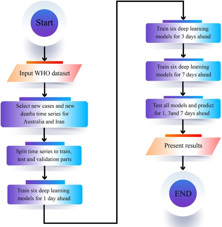
During the training for the first time, the time series were fed to the model based on which the model predicted the next day. The model training was repeated for the second time such that its output predicted the next three days. Finally, the model was trained for the third time to achieve predictions for the next seven days. As the forecasting horizon increases from one to three and to seven, the error rate of the model increases, which makes sense since forecasting for a longer horizon is harder than forecasting for a shorter horizon. The training process was implemented for both the time series of new cases and new deaths. Fig. 1 illustrates the high-level steps of the proposed method.
Fig. 1.
The proposed method high-level steps.
Experimental results and analysis
In this section, the experimental results for LSTM, Conv-LSTM and GRU, as well as their bidirectional counterparts, are reported. To the best of our knowledge, we are the first to use Bi-Conv-LSTM and Bi-GRU for the prediction of COVID-19 new cases and deaths based on time series data.
To have a fair comparison, we tried to implement all methods with relatively similar conditions. The prediction error was calculated based on criteria [14] such as Mean Squared Log Error (MSLE), Mean Absolute Percentage Error (MAPE), Root Mean Squared Log Error (RMSLE), and Explained Variance (EV). These evaluation criteria are computed as below [41]:
| (1) |
| (2) |
| (3) |
| (4) |
where is the actual values, is the corresponding estimated values, and n is the number of samples.
Forecasting performance
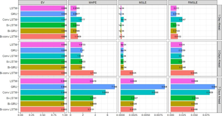
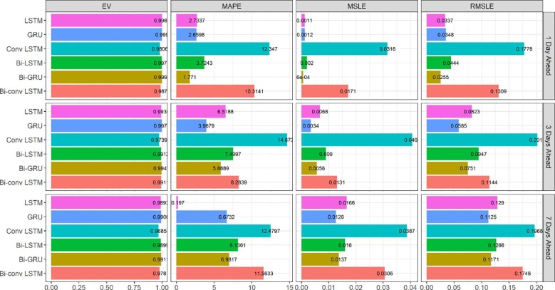
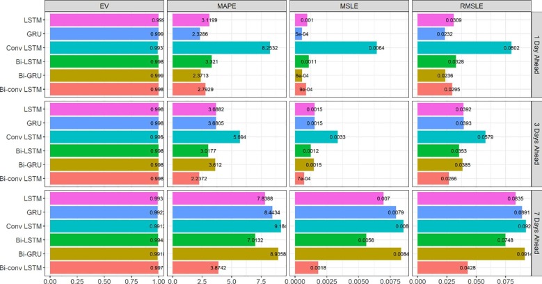
For each of the mentioned methods, the error of 1, 3, and 7-day ahead predictions for new cases/deaths in a 100-day period were calculated in Australia and Iran. To this end, the predicted values were compared with the actual values, and the error rate was calculated based on evaluation criteria (Equations 1–4). The results of calculating the errors in the 100-day period for each of Australia’s models are given in Fig. 2 and Fig. 3 . As it is apparent from MAPE values in Fig. 2, Bi-GRU and LSTM have the best performance in the 1-day prediction, Conv-LSTM is the best method in the 3-day prediction, and Bi-Conv-LSTM has the best performance in the 7-day prediction. All of the evaluated methods in Fig. 2 have approximately similar explained variance. Fig. 3 illustrates the evaluation results for new deaths prediction for the 100-day period in Australia. An interesting observation in Fig. 3 is how LSTM significantly outperforms GRU in the 7-day ahead prediction. The reason lies in the fact that GRU has a simpler structure (fewer parameters) consisting of only two gates. However, the more complex structure of LSTM seems to prevail sometimes, as is the case in the 7-day prediction of new deaths in Fig. 3.
Fig. 2.
Evaluation metrics for new cases forecasting in Australia.
Fig. 3.
Evaluation metrics for new deaths forecasting in Australia.
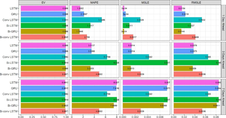
The evaluation results of the models for the prediction of Iran new cases and new deaths are presented in Fig. 4, Fig. 5 . The main observation based on the MAPE criterion in these figures is that most of the time, LSTM and its variations outperform GRU, especially for the longer horizons (3 and 7-day) scenarios.
Fig. 4.
Evaluation metrics for new cases forecasting in Iran.
Fig. 5.
Evaluation metrics for new deaths forecasting in Iran.
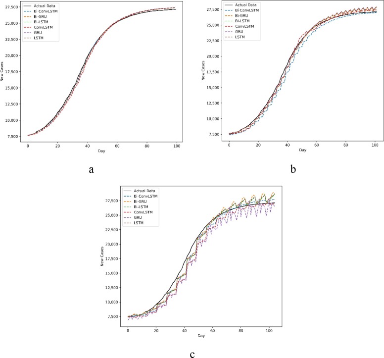
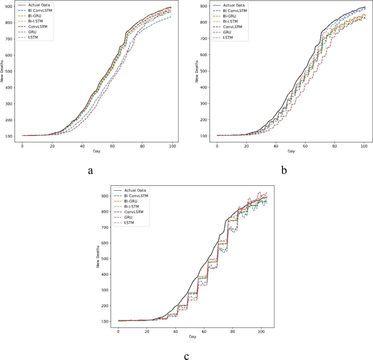
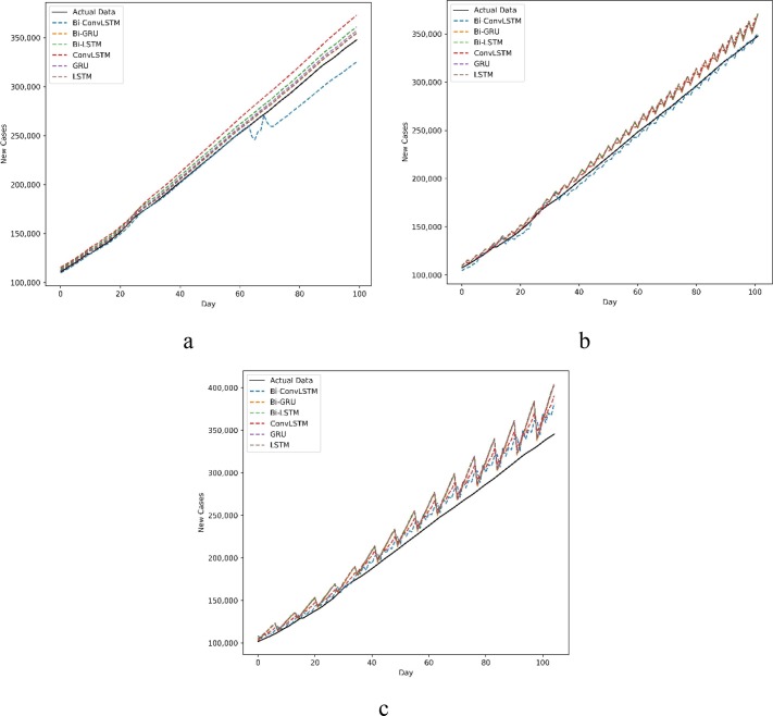
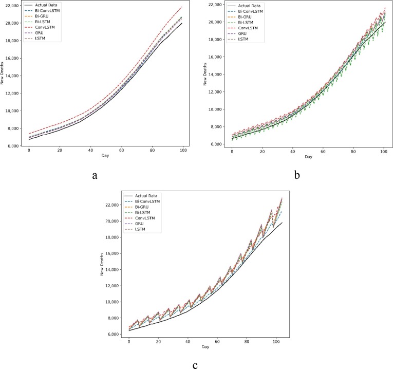
The predictions of new cases and new deaths in Australia and Iran for 1, 3, and 7-day ahead are compared with actual data in Fig. 6, Fig. 7, Fig. 8, Fig. 9 . The prevalent pattern observed in these figures is that a longer prediction horizon often leads to larger prediction errors. Of course, such a pattern is violated in Fig. 8.a where Bi-Conv-LSTM has deviated from the actual data badly.
Fig. 6.
New cases forecasting a) every day, b) every 3 d and c) every 7 d in Australia.
Fig. 7.
New deaths forecasting a) every day, b) every 3 d and c) every 7 d in Australia.
Fig. 8.
New cases forecasting a) every day, b) every 3 d and c) every 7 d in Iran.
Fig. 9.
New deaths forecasting a) every day, b) every 3 d, and c) every 7 d in Iran.
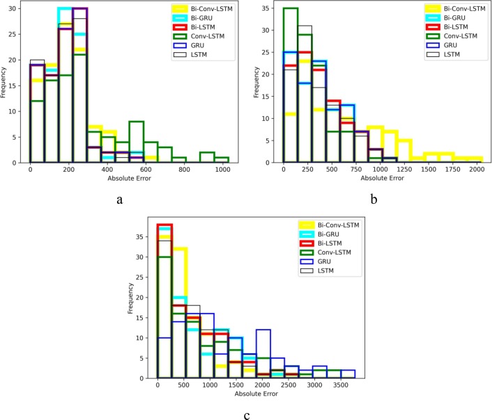
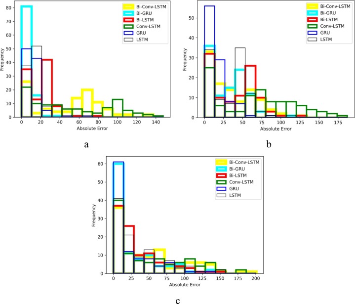
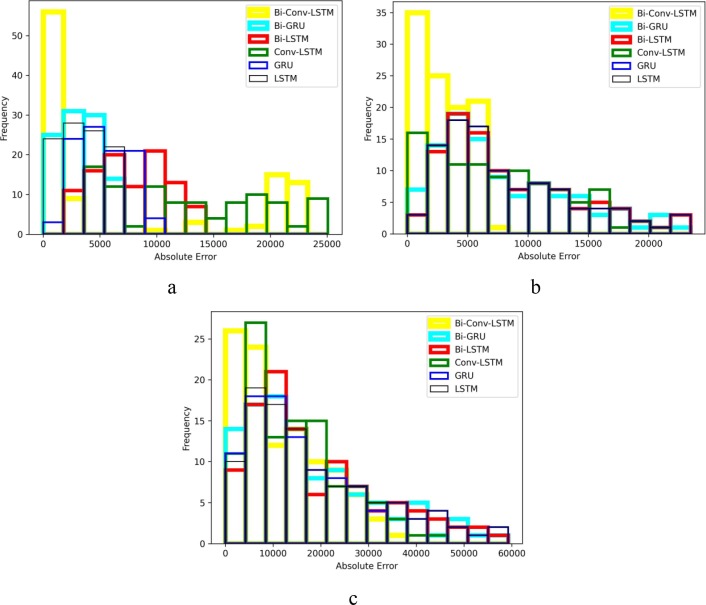
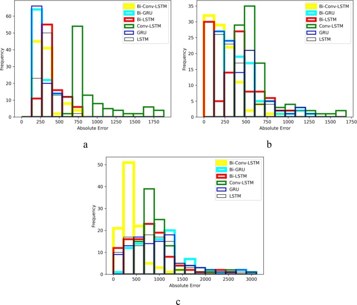
For a better comparison of the six methods performance, histograms of their absolute error are also presented in Fig. 10, Fig. 11, Fig. 12, Fig. 13 . The horizontal axes of the histograms represent the absolute error which is the difference between the models predictions and the actual data. Recall that predictions are performed for 100 days. The height of each histogram bin shows the number of predictions in which absolute error falls within the interval dictated by that bin. For better clarity, in Fig. 10, Fig. 11, Fig. 12, Fig. 13, the histograms of different methods are drawn with different colours and line widths. At first glance, the maximum absolute error observed in Fig. 10, Fig. 11, Fig. 12, Fig. 13 seems to be too high. However, it should be noted that the number of new cases/deaths each day are cumulative values. In other words, the actual new cases/deaths reported for i-th day is the total number of new cases/deaths reported from the first day until i-th day across the whole country (such as Iran). Considering that data are reported as cumulative values, it comes as no surprise that they are usually large values. The absolute error of prediction is directly influenced by the magnitude of the actual data. For example, in a one-day prediction of new cases for Iran (Fig. 12.a), GRU has predicted 354,000 while the true value was 345,000. The absolute error in this case is which is 2.6% of the true value. At first, 9,000 seems to be a large error, but it is indeed tolerable compared to the magnitude of the true value (345,000). For the seven days ahead prediction (Fig. 12.c), the same method has predicted 404,000 while the true value was 345,000. The absolute error is which is 17.10% of the true value. Obviously, the absolute error of the seven days ahead prediction is higher than that of one day ahead prediction. However, 59,000 is still a reasonable value compared to the true value.
Fig. 10.
Absolute error histogram of forecasting new cases in Australia a) every day, b) every 3 d and c) every 7 d.
Fig. 11.
Absolute error histogram of forecasting new deaths in Australia a) every day, b) every 3 d and c) every 7 d.
Fig. 12.
Absolute error histogram of forecasting new cases in Iran a) every day, b) every 3 d, and c) every 7 d.
Fig. 13.
Absolute error histogram of forecasting new deaths in Iran a) every day, b) every 3 d and c) every 7 d.
Statistical analysis
Friedman [43] proposed a nonparametric statistical test known as the Friedman test [44], which is widely used by researchers to analyse their methods [45]. In this subsection, the Friedman test was used to compare the algorithms. To this end, the average of error evaluation criteria (EV, MAPE, MSLE, RMSLE) in Fig. 2, Fig. 3, Fig. 4, Fig. 5 were computed and listed in Table 3 , based on which the algorithms were ranked as shown in Table 4 . The methods with lower ranks are better than the ones with higher ranks.
Table 3.
Average of error evaluation metrics.
| Dataset | LSTM | GRU | Conv-LSTM | Bi-LSTM | Bi-GRU | Bi-Conv-LSTM |
|---|---|---|---|---|---|---|
| New Cases 1-day AU | 0.49265 | 0.494675 | 0.71 | 0.49435 | 0.4927 | 0.548825 |
| New Cases 3-day AU | 0.723475 | 0.732625 | 0.66365 | 0.72595 | 0.71915 | 1.19685 |
| New Cases 7-day AU | 1.170475 | 2.074175 | 1.691325 | 1.18285 | 1.1824 | 1.0894 |
| New Deaths 1-day AU | 0.941625 | 0.9237 | 3.38425 | 1.191925 | 0.699025 | 2.862275 |
| New Deaths 3-day AU | 1.900225 | 1.2567 | 3.971975 | 2.14865 | 1.7409 | 2.3506 |
| New Deaths 7-day AU | 0.33295 | 1.947175 | 3.420925 | 2.317075 | 2.025875 | 3.186675 |
| New Cases 1-day IR | 0.6287 | 0.7975 | 1.594025 | 1.083375 | 0.6021 | 0.93275 |
| New Cases 3-day IR | 1.136925 | 1.135425 | 1.8335 | 2.269875 | 1.088375 | 1.476 |
| New Cases 7-day IR | 2.275075 | 2.24805 | 1.8335 | 2.269875 | 2.124775 | 1.476 |
| New Deaths 1-day IR | 1.0377 | 0.852075 | 2.3332 | 1.088225 | 0.848625 | 0.955325 |
| New Deaths 3-day IR | 1.181725 | 1.179825 | 1.6878 | 1.01305 | 1.1625 | 0.815625 |
| New Deaths 7-day IR | 2.230575 | 2.3831 | 2.56875 | 2.0219 | 2.50665 | 1.22895 |
Table 4.
Rank of the algorithms on datasets.
| Dataset | LSTM | GRU | Conv-LSTM | Bi-LSTM | Bi-GRU | Bi-Conv-LSTM |
|---|---|---|---|---|---|---|
| New Cases 1-day AU | 1 | 4 | 6 | 3 | 2 | 5 |
| New Cases 3-day AU | 3 | 5 | 1 | 4 | 2 | 6 |
| New Cases 7-day AU | 2 | 6 | 3 | 5 | 4 | 1 |
| New Deaths 1-day AU | 3 | 2 | 6 | 4 | 1 | 5 |
| New Deaths 3-day AU | 3 | 1 | 6 | 4 | 2 | 5 |
| New Deaths 7-day AU | 1 | 2 | 6 | 4 | 3 | 5 |
| New Cases 1-day IR | 2 | 3 | 5 | 5 | 1 | 4 |
| New Cases 3-day IR | 3 | 2 | 1 | 6 | 1 | 4 |
| New Cases 7-day IR | 6 | 4 | 6 | 5 | 3 | 1 |
| New Deaths 1-day IR | 4 | 2 | 6 | 5 | 1 | 3 |
| New Deaths 3-day IR | 5 | 4 | 6 | 2 | 3 | 1 |
| New Deaths 7-day IR | 3 | 4 | 6 | 2 | 5 | 1 |
| Average Rank | 3 | 3.25 | 4.83 | 4.08 | 2.33 | 3.42 |
To carry out the Friedman test, the rankings from Table 4 are required. Suppose the rank of the j-th classifier on the i-th dataset is denoted by ri j so the average rank of the algorithms can be computed by . The Friedman test is then computed by the following formula:
| (5) |
where k is the number of algorithms and N is the number of datasets. Motivated by the Friedman test, Iman and Davenport [46] proposed another statistical test as follows:
| (6) |
which has F-distribution with ((k − 1),(k − 1)(N − 1)) degrees of freedom. According to the results of Table 4, χ2 F and Ff are computed as follows:
According to six algorithms and 12 datasets (New cases 1-day AU, …), is governed by the F-distribution with ((k − 1), (k − 1)(N − 1)) = (5,55) degree of freedom. The critical value of F(5,55) is 2.38 for significance level α = 0.05. As it is clear in Table 4, the Bi-GRU algorithm has the best average rank among all the algorithms followed by LSTM, GRU, Bi-Conv-LSTM, Bi-LSTM, and Conv-LSTM.
Discussion
Time series prediction is an important topic in finance, economics, and business. Recent advancement in computers’ computational power, ML methods and new perspectives such as DL have led to the emergence of new algorithms for times series analysis and prediction. Some of these algorithms are LSTM, GRU, Conv-LSTM, Bi-LSTM, Bi-GRU and Bi-Conv-LSTM. Each algorithm has its advantages and disadvantages. Our investigation about the forecasting ability of these methods on the COVID-19 time series led to the following contributions:
-
•
Based on the literature review, it seems that Bi-GRU and Bi-Conv-LSTM models have never been used before for prediction on COVID-19 new cases and new deaths rate time series.
-
•
No research was found which predicts new cases and new deaths every three or seven days. The motivation behind attempting to predict every n days (instead of every day) was to investigate whether it is possible to reduce computational complexity and still achieve reasonable performance. Such a scenario gains importance in any application involving real-time forecasting of time series. Whether the incurred error due to prediction every n days is acceptable or not fully depends on the application requirements. It is the designer who decides whether it is worth sacrificing performance to gain better computation efficiency. In our experiments, an inspection of the RMSLE metric in Fig. 2, Fig. 3, Fig. 4, Fig. 5 shows that predicting every three days approximately doubles the prediction error. The incurred error of predicting every seven days is more than four times of error when prediction is made every day.
-
•
A comprehensive evaluation of LSTM, Conv-LSTM, GRU and their bidirectional extensions.
-
•
Statistical comparison of the investigated methods using Friedman test.
Recall that in Fig. 2, Fig. 3, Fig. 4, Fig. 5, the error rate of the new cases and new deaths in Iran and Australia were determined by methods LSTM, GRU, Conv-LSTM, Bi-LSTM, Bi-GRU and Bi-Conv-LSTM. Overall, it was observed that in most of the conducted experiments (Fig. 2, Fig. 3, Fig. 4, Fig. 5), the bidirectional methods achieved better results than the other methods.
Based on data in Table 4, the key observations can be summarised as below:
-
•
For the prediction of new deaths in the next day in Australia and Iran, Bi-GRU had the best performance. For 3-d ahead prediction of new deaths in Australia, GRU was the best method, while Bi-Conv-LSTM made the best prediction in Iran. Finally, in the 7-d ahead case, LSTM performed better than other methods on Australia data, and Bi-Conv-LSTM outperformed other methods on Iran data.
-
•
On the other hand, for 1-d ahead predictions of new cases in Australia, LSTM and Bi-GRU gained the best performance. For 3 and 7-d ahead predictions, Conv-LSTM and Bi-Conv-LSTM showed better performance, respectively. In Iran, Bi-GRU was better for 1 and 3-d ahead predictions, and Bi-Conv-LSTM was better for 7-d ahead prediction.
The proposed method can provide the health crisis management centres with valuable forecasting based on the observed data. Having an estimate of what awaits us in the near future might help with the appropriate preparation to minimise the inevitable damage. The forecasting ability of the six models is due to their memorising capability. The limitation of the proposed method is that the characteristics of the time series data might change as time passes. Therefore, to keep the models accurate, we are forced to incur the cost of training the models on the newly observed data.
Conclusion
In this research, six different models were compared for predicting the number of new cases and deaths in the next 100 d. The prediction was made for each day, every 3 d and every 7 d. The conducted experiments showed that most of the time, the bidirectional models outperform their non-bidirectional counterparts.
In the future research, the plan is to use a combination of other machine learning and deep learning methods to achieve better results. In particular, experimenting with nonparametric models such as Gaussian Process (GP) to perform time series forecasting seems interesting since GP can provide uncertainty about its predictions. We might be able to determine the appropriate prediction horizon based on the uncertainty provided by GP.
CRediT authorship contribution statement
Nooshin Ayoobi: Conceptualization, Data curation, Formal analysis, Investigation, Methodology, Validation, Writing - original draft. Danial Sharifrazi: Conceptualization, Data curation, Formal analysis, Investigation, Methodology, Validation, Writing - original draft. Roohallah Alizadehsani: Formal analysis, Methodology, Writing - original draft. Afshin Shoeibi: Formal analysis, Methodology, Writing - original draft. Juan M. Gorriz: Validation, Conceptualization, Investigation. Hossein Moosaei: Formal analysis, Methodology, Writing - original draft. Abbas Khosravi: Conceptualization, Methodology, Project administration. Saeid Nahavandi: Conceptualization, Methodology, Project administration. Abdoulmohammad Gholamzadeh Chofreh: Formal analysis, Methodology, Writing - original draft. Feybi Ariani Goni: Formal analysis, Methodology, Writing - original draft. Jiří Jaromír Klemeš: Methodology, Resources, Project administration, Writing - review & editing. Amir Mosavi: .
Declaration of Competing Interest
The authors declare that they have no known competing financial interests or personal relationships that could have appeared to influence the work reported in this paper.
Acknowledgements
Several researchers benefited from the EU supported project Sustainable Process Integration Laboratory — SPIL funded as project No. CZ.02.1.01/0.0/0.0/15_003/0000456, by Czech Republic Operational Programme Research and Development, Education, Priority 1: Strengthening capacity for quality research, based on the SPIL project. This work was also partly supported by the Ministerio de Ciencia e Innovación (España)/ FEDER under the RTI2018-098913-B100 project, by the Consejería de Economía, Innovación, Ciencia y Empleo (Junta de Andalucía) and FEDER under CV20-45250 and A-TIC-080-UGR18 projects.
References
- 1.Alizadehsani R., Alizadeh Sani Z., Behjati M., Roshanzamir Z., Hussain S., Abedini N. Risk factors prediction, clinical outcomes, and mortality in COVID-19 patients. J Med Virol. 2021;93(4):2307–2320. doi: 10.1002/jmv.26699. [DOI] [PMC free article] [PubMed] [Google Scholar]
- 2.Eskandarian R., Sani Z.A., Behjati M., Zahmatkesh M., Haddadi A., Kakhi K. Identification of clinical features associated with mortality in COVID-19 patients. medRxiv. 2021 [Google Scholar]
- 3.Sharifrazi D., Alizadehsani R., Roshanzamir M., Joloudari J.H., Shoeibi A., Jafari M. Fusion of convolution neural network, support vector machine and Sobel filter for accurate detection of COVID-19 patients using X-ray images. Biomed Signal Process Control. 2021;68:102622. doi: 10.1016/j.bspc.2021.102622. [DOI] [PMC free article] [PubMed] [Google Scholar]
- 4.Chan J.-W., Yuan S., Kok K.-H., To K.-W., Chu H., Yang J. A familial cluster of pneumonia associated with the 2019 novel coronavirus indicating person-to-person transmission: a study of a family cluster. The Lancet. 2020;395(10223):514–523. doi: 10.1016/S0140-6736(20)30154-9. [DOI] [PMC free article] [PubMed] [Google Scholar]
- 5.Javan A.A.K., Jafari M., Shoeibi A., Zare A., Khodatars M., Ghassemi N. Medical Images Encryption Based on Adaptive-Robust Multi-Mode Synchronization of Chen Hyper-Chaotic Systems. Sensors. 2021;21(11):3925. doi: 10.3390/s21113925. [DOI] [PMC free article] [PubMed] [Google Scholar]
- 6.Burke RM. Active monitoring of persons exposed to patients with confirmed COVID-19—United States, January–February 2020. MMWR Morbidity and mortality weekly report. 2020;69. [DOI] [PMC free article] [PubMed]
- 7.Shoeibi A, Khodatars M, Alizadehsani R, Ghassemi N, Jafari M, Moridian P, et al. Automated detection and forecasting of covid-19 using deep learning techniques: A review. arXiv preprint arXiv:200710785. 2020.
- 8.Fanelli D., Piazza F. Analysis and forecast of COVID-19 spreading in China, Italy and France. Chaos, Solitons Fractals. 2020;134:109761. doi: 10.1016/j.chaos.2020.109761. [DOI] [PMC free article] [PubMed] [Google Scholar]
- 9.Rothe C., Schunk M., Sothmann P., Bretzel G., Froeschl G., Wallrauch C. Transmission of 2019-nCoV Infection from an Asymptomatic Contact in Germany. N Engl J Med. 2020;382(10):970–971. doi: 10.1056/NEJMc2001468. [DOI] [PMC free article] [PubMed] [Google Scholar]
- 10.Hunter D.J. Covid-19 and the Stiff Upper Lip — The Pandemic Response in the United Kingdom. N Engl J Med. 2020;382(16):e31. doi: 10.1056/NEJMp2005755. [DOI] [PubMed] [Google Scholar]
- 11.Gautret P., Lagier J.-C., Parola P., Hoang V.T., Meddeb L., Mailhe M. Hydroxychloroquine and azithromycin as a treatment of COVID-19: results of an open-label non-randomised clinical trial. Int J Antimicrob Agents. 2020;56(1) doi: 10.1016/j.ijantimicag.2020.105949. [DOI] [PMC free article] [PubMed] [Google Scholar] [Retracted]
- 12.Takian A., Raoofi A., Kazempour-Ardebili S. COVID-19 battle during the toughest sanctions against Iran. Lancet. 2020;395(10229):1035–1036. doi: 10.1016/S0140-6736(20)30668-1. [DOI] [PMC free article] [PubMed] [Google Scholar]
- 13.World Health Organization, WHO Coronavirus Disease (COVID-19) Dashboard. https://covid19.who.int/ (accessed on 13 May 2021).
- 14.Zeinalnezhad M., Chofreh A.G., Goni F.A., Klemeš J.J., Sari E. Simulation and Improvement of Patients’ Workflow in Heart Clinics during COVID-19 Pandemic Using Timed Coloured Petri Nets. Int J Environ Res Public Health. 2020;17(22):8577. doi: 10.3390/ijerph17228577. [DOI] [PMC free article] [PubMed] [Google Scholar]
- 15.Khozeimeh F, Sharifrazi D, Izadi NH, Joloudari JH, Shoeibi A, Alizadehsani R, et al. CNN AE: Convolution Neural Network combined with Autoencoder approach to detect survival chance of COVID 19 patients. arXiv preprint arXiv:210408954. 2021. [DOI] [PMC free article] [PubMed]
- 16.Asgharnezhad H, Shamsi A, Alizadehsani R, Khosravi A, Nahavandi S, Sani ZA, et al. Objective Evaluation of Deep Uncertainty Predictions for COVID-19 Detection. arXiv preprint arXiv:201211840. 2020. [DOI] [PMC free article] [PubMed]
- 17.Górriz J.M., Ramírez J., Ortíz A., Martínez-Murcia F.J., Segovia F., Suckling J. Artificial intelligence within the interplay between natural and artificial computation: Advances in data science, trends and applications. Neurocomputing. 2020;410:237–270. [Google Scholar]
- 18.Alizadehsani R, Sharifrazi D, Izadi NH, Joloudari JH, Shoeibi A, Gorriz JM, et al. Uncertainty-aware semi-supervised method using large unlabelled and limited labeled COVID-19 data. arXiv preprint arXiv:210206388. 2021.
- 19.Pinter G., Felde I., Mosavi A., Ghamisi P., Gloaguen R. COVID-19 Pandemic Prediction for Hungary; a Hybrid Machine Learning Approach. Mathematics. 2020;8(6):890. [Google Scholar]
- 20.Worldometers, Hungary Coronavirus Cases, <https://www.worldometers.info/coronavirus/country/hungary/> (accessed on 1 June 2021).
- 21.Dowd J.B., Andriano L., Brazel D.M., Rotondi V., Block P., Ding X. Demographic science aids in understanding the spread and fatality rates of COVID-19. Proc Natl Acad Sci. 2020;117(18):9696–9698. doi: 10.1073/pnas.2004911117. [DOI] [PMC free article] [PubMed] [Google Scholar]
- 22.Arun SS, Iyer GN, editors. On the Analysis of COVID19 - Novel Corona Viral Disease Pandemic Spread Data Using Machine Learning Techniques. 2020 4th International Conference on Intelligent Computing and Control Systems (ICICCS); 2020 13-15 May 2020.
- 23.Zeroual A., Harrou F., Dairi A., Sun Y. Deep learning methods for forecasting COVID-19 time-Series data: A Comparative study. Chaos, Solitons Fractals. 2020;140:110121. doi: 10.1016/j.chaos.2020.110121. [DOI] [PMC free article] [PubMed] [Google Scholar]
- 24.Babaei A., Jafari H., Banihashemi S., Ahmadi M. Mathematical analysis of a stochastic model for spread of Coronavirus. Chaos, Solitons Fractals. 2021;145:110788. doi: 10.1016/j.chaos.2021.110788. [DOI] [PMC free article] [PubMed] [Google Scholar]
- 25.Babaei A., Ahmadi M., Jafari H., Liya A. A mathematical model to examine the effect of quarantine on the spread of Coronavirus. Chaos, Solitons Fractals. 2021;142:110418. doi: 10.1016/j.chaos.2020.110418. [DOI] [PMC free article] [PubMed] [Google Scholar]
- 26.Babaei A., Jafari H., Banihashemi S., Ahmadi M. A stochastic mathematical model for COVID-19 according to different age groups. Applied and Computational Mathematics. 2021;20(1):140–159. [Google Scholar]
- 27.Danane J., Allali K., Hammouch Z., Nisar K.S. Mathematical analysis and simulation of a stochastic COVID-19 Lévy jump model with isolation strategy. Results Phys. 2021;23:103994. doi: 10.1016/j.rinp.2021.103994. [DOI] [PMC free article] [PubMed] [Google Scholar]
- 28.Wu L.-I., Feng Z. Homoclinic Bifurcation in an SIQR Model for Childhood Diseases. Journal of Differential Equations. 2000;168(1):150–167. [Google Scholar]
- 29.Ministère de la Santé, 2021, Corona, <https://www.sante.gov.ma/Pages/corona.aspx> (accessed on 24 May 2021).
- 30.World Health Organization, 2021, WHO Coronavirus (COVID-19) Dashboard, <https://covid19.who.int/> (accessed on 28 June 2021).
- 31.Singh H., Srivastava H.M., Hammouch Z., Sooppy Nisar K. Numerical simulation and stability analysis for the fractional-order dynamics of COVID-19. Results Phys. 2021;20:103722. doi: 10.1016/j.rinp.2020.103722. [DOI] [PMC free article] [PubMed] [Google Scholar]
- 32.Gao W., Veeresha P., Prakasha D.G., Baskonus H.M. Novel Dynamic Structures of 2019-nCoV with Nonlocal Operator via Powerful Computational Technique. Biology. 2020;9(5):107. doi: 10.3390/biology9050107. [DOI] [PMC free article] [PubMed] [Google Scholar]
- 33.Gao W., Veeresha P., Baskonus H.M., Prakasha D.G., Kumar P. A new study of unreported cases of 2019-nCOV epidemic outbreaks. Chaos, Solitons Fractals. 2020;138:109929. doi: 10.1016/j.chaos.2020.109929. [DOI] [PMC free article] [PubMed] [Google Scholar]
- 34.Boudaoui A., El hadj Moussa Y., Hammouch Z., Ullah S. A fractional-order model describing the dynamics of the novel Coronavirus (COVID-19) with nonsingular kernel. Chaos, Solitons Fractals. 2021;146:110859. doi: 10.1016/j.chaos.2021.110859. [DOI] [PMC free article] [PubMed] [Google Scholar]
- 35.Tang B., Wang X., Li Q., Bragazzi N.L., Tang S., Xiao Y. Estimation of the Transmission Risk of the 2019-nCoV and Its Implication for Public Health Interventions. Journal of Clinical Medicine. 2020;9(2):462. doi: 10.3390/jcm9020462. [DOI] [PMC free article] [PubMed] [Google Scholar]
- 36.Zamir M., Nadeem F., Abdeljawad T., Hammouch Z. Threshold condition and non pharmaceutical interventions’s control strategies for elimination of COVID-19. Results Phys. 2021;20:103698. doi: 10.1016/j.rinp.2020.103698. [DOI] [PMC free article] [PubMed] [Google Scholar]
- 37.Sahoo P., Mondal H.S., Hammouch Z., Abdeljawad T., Mishra D., Reza M. On the necessity of proper quarantine without lock down for 2019-nCoV in the absence of vaccine. Results Phys. 2021;25:104063. doi: 10.1016/j.rinp.2021.104063. [DOI] [PMC free article] [PubMed] [Google Scholar]
- 38.Gao W., Baskonus H.M., Shi L. New investigation of bats-hosts-reservoir-people coronavirus model and application to 2019-nCoV system. Advances in Difference Equations. 2020;2020(1):391. doi: 10.1186/s13662-020-02831-6. [DOI] [PMC free article] [PubMed] [Google Scholar]
- 39.Wang L, Xu X, Dong H, Gui R, Yang R, Pu F, editors. Exploring Convolutional Lstm for Polsar Image Classification. IGARSS 2018 - 2018 IEEE International Geoscience and Remote Sensing Symposium; 2018 22-27 July 2018.
- 40.Dey R, Salem FM, ed. Gate-variants of Gated Recurrent Unit (GRU) neural networks. 2017 IEEE 60th International Midwest Symposium on Circuits and Systems (MWSCAS); 2017 6-9 Aug. 2017.
- 41.Di Persio L., Honchar O. Artificial neural networks architectures for stock price prediction: Comparisons and applications. International Journal of Circuits, Systems and Signal Processing. 2016;2016(10):403–413. [Google Scholar]
- 42.World Health Organization, WHO Coronavirus Disease (COVID-19) Dashboard. https://covid19.who.int/table (accessed 10 May 2021).
- 43.Daniel W.W. Friedman two-way analysis of variance by ranks. Applied Nonparametric. Statistics. 1990:262–274. [Google Scholar]
- 44.Friedman M. A comparison of alternative tests of significance for the problem of m rankings. Ann Math Stat. 1940;11(1):86–92. [Google Scholar]
- 45.Bazikar F., Ketabchi S., Moosaei H. DC programming and DCA for parametric-margin ν-support vector machine. Applied Intelligence. 2020;50(6):1763–1774. [Google Scholar]
- 46.Iman R.L., Davenport J.M. Approximations of the critical region of the fbietkan statistic. Communications in Statistics-Theory and Methods. 1980;9(6):571–595. [Google Scholar]


