A brief introduction to the analysis of time-series data from biologging studies

Abstract

Recent advances in tagging and biologging technology have yielded unprecedented insights into wild animal physiology. However, time-series data from such wild tracking studies present numerous analytical challenges owing to their unique nature, often exhibiting strong autocorrelation within and among samples, low samples sizes and complicated random effect structures. Gleaning robust quantitative estimates from these physiological data, and, therefore, accurate insights into the life histories of the animals they pertain to, requires careful and thoughtful application of existing statistical tools. Using a combination of both simulated and real datasets, I highlight the key pitfalls associated with analysing physiological data from wild monitoring studies, and investigate issues of optimal study design, statistical power, and model precision and accuracy. I also recommend best practice approaches for dealing with their inherent limitations. This work will provide a concise, accessible roadmap for researchers looking to maximize the yield of information from complex and hard-won biologging datasets.

This article is part of the theme issue ‘Measuring physiology in free-living animals (Part II)’.

1. Introduction

Biologging technology allows us to study the physiology and behaviour of wildlife in unprecedented detail [1], particularly for cryptic and elusive species [2,3]. In addition to host-specific metrics like heart rate [4–7], brain activity [8] and movement behaviour [9–12], biologging can also gather information about the abiotic environment experienced by the host (e.g. [11,13]). These data can also be used to understand how individual performance is influenced by environmental variation and/or extremes, and potentially to predict how animals may respond to climate change (see Chmura et al. [14]). The diverse plethora of data that can be gathered from a single device mean that biologging studies are extremely information-rich, perhaps containing thousands of data points for each measured variable (e.g. [15–17]). However, this high per-device information content comes at a cost. Data analysis is complicated by the fact that resulting datasets are often time series, where successive values of our metrics of interests are dependent on values from prior sampling events [18] (table 1). For example, the blood pO₂ of a diving elephant seal at time t during a dive is entirely dependent on pO₂ at time t − 1 because of a limited store of oxygen [34]; or, trends in body temperature over time may be non-random because of circadian rhythms [35,36]. This distinction is important because it changes some decisions we might make about how we conduct our analyses. To glean some insight from our hard-won biologging data, not only do we need to draw on the ‘standard’ statistical toolkit that physiologists are expected to be familiar with, including general(ized) linear models, their mixed model equivalents [37] and their potential pitfalls [38,39], but we also need to equip ourselves with the skills necessary to deal with time series [18,40]. Testing hypotheses about the processes driving variation in our data requires that we design biologging studies carefully and apply these tools correctly [41].

Table 1.

Examples of some physiological biologging data that are likely to be temporally autocorrelated (i.e. that successive values are probably dependent on prior values) if used serially, and, therefore, should be treated with consideration. (Also shown are recent example use-cases to illustrate what data from each variable tend to look like, with no reference made to the statistical treatment of the data in each study.)

variable	Reason	use-cases
electrocardiogram (ECG)	latency in cardiovascular response sampling frequency usually very high (e.g. 100–180 Hz) compared to cardiovascular response	Bishop et al. [19], Hawkes et al. [4], Elmegaard et al. [20]
electroencephalogram (EEG)	sampling frequency usually very high (e.g. 200 Hz), compared to physiological response to stimuli (e.g. light at night) or events such as migration, navigation or sleep. Some neural responses may have functional long-term correlations [21].	Rattenborg et al. [22], Vyssotski et al. [23], Voirin et al. [24]
body temperature	core body temperature usually changes slowly owing to thermal inertia	Parr et al. [25], Streicher et al. [26], Hume et al. [27]
blood pO2	during a dive underwater, finite O2 store (i.e. total O2 decreases, although regional compression hyperoxia can occur) depending on extent of desaturation, latency in fully reoxygenating haemoglobin	Meir et al. [28], Stockard et al. [29], Williams & Hicks [30]
accelerometry	dynamic inertia (e.g. during flight, running or falling)	Whitney et al. [31], Van Walsum et al. [32], Fehlmann et al. [33]

The problem is that it is not always clear which models to apply to our data, nor if we can trust the numbers that come out of those models, though, of course, this issue is pervasive throughout statistical sciences (e.g. [37,42,43]). The goal of this paper is to provide an accessible guide to those setting out into the world of biologging data analysis for studies of animal physiology. I discuss some common pitfalls of time-series analysis, and use simulations of various biologging data types to stress-test common modelling frameworks to determine when parameter estimates are robust, and so can form a solid foundation for hypothesis testing and biological inference. Particular attention is given to the issue of small sample sizes, and how model estimates are affected when the total number of individuals in a study is small. All data, analyses, plotting and simulations in this paper are provided as a reproducible RMarkdown document, built in the software R [44] using a variety of data manipulation, modelling and plotting packages [45–53].

(a) . A brief primer on time-series modelling for biologging studies

The field of biologging is vast, and growing [9,10]. Researchers have an enormous diversity of sensors and devices at their disposal that can be attached to their organisms of interest, and the types of questions they might be interested in tackling is equally varied (see table 1 in [41]). Addressing how to model all of these data types to tackle a broad array of questions is beyond the scope of this review, but we can deal with some common rules. For example, it might be the case that you want to use your data to classify or count the frequency of a certain behaviour, such as heart rate dropping below a lower threshold during a dive [54]. In such cases, extracting derived variables from the time series allows you to work comfortably in the realm of ‘standard’ tools such as general linear models (GLMs) and their mixed effect counterparts to model count processes [37]. This is because you are condensing a time series of logger data into what is essentially a summary statistic. A good rule of thumb here is that if each logger/individual is only ‘contributing’ a single data point to the models (from a time series containing potentially thousands of observations), you are probably safe. However, arriving at those summary statistics can often be challenging, and require some more sophisticated modelling tools (see the ‘Beyond simple autocorrelation structures' section). Here, we will first address the workflow for fitting, assessing and interpreting autocorrelation models of biologging data and the time series that biologging devices yield.

When we first set out to model raw time series from biologging devices, a very simple directive is never to use t-tests or ‘ordinary’ GLMs to analyse data that show clear temporal trends. Some of you reading this might think it is too obvious a statement to warrant making, but such an approach is still widely used even among established researchers. These simulations evidence that doing so greatly inflates the risk of Type I error, which is something we strongly wish to avoid. To demonstrate, this we can examine some hypothetical logger data from two Velociraptor mongoliensis individuals (figure 1a). The important thing to know about these hypothetical data is that the data-generating process for both is identical—both have the same mean (μ = 0) and neither show any temporal trends in the mean logger value. Note that this is different from there being no signature of temporal autocorrelation in the data (more on this below). Thus, we expect that any statistical test should show us no difference between individuals in mean, and no trend over time. But if we pick our statistical tests poorly, this is exactly what we get. Over 1000 simulations, a simple t-test for difference between means of the two logger traces yields a significant result (Type I error rate) 25.5% of the time (figure 1b), way above the 5% nominal α. Using a GLM for the same test yields similar results, as does asking if there is a temporal trend (figure 1b). Only by using a model that accounts for the temporal autocorrelation, in this case, a generalized least squares (GLS) model, can we control the Type I error rate at the 5% level for the effect of time (figure 1b).

Figure 1.

The effect of model specification on rates of Type I error when investigating differences in biologging data taken from two V. mongoliensis individuals. (a) Time-series traces of physiological measurements of two individual Velociraptors with identical means (μ = 0) and data-generating processes (AR1, rho = 0.5). (b) Densities of p-values from 1000 replicate iterations of data generation. Panel labels refer to analytical model (e.g. GLM) followed by term being tested (e.g. identification (ID)). Both GLMs and t-tests incorrectly estimate a significant difference between individuals in roughly 25% of simulations, well above the nominal α = 0.05. GLMs also incorrectly estimate a significant trend over time in greater than 25% of cases. Only GLS models accounting for temporal autocorrelation show the expected uniform distribution of p-values compatible with a Type I error rate controlled at 5%.

There are many types of physiological data that require we model serial correlation and heterogeneity (table 1). Likewise, there is a large range of flexible tools that allow us to deal with these two traits of biologging data. For example, heterogeneity might manifest in Gaussian models where the variance is not constant with the mean, as well as cases where the residuals are non-independent. Both can be present in biologging data, but the latter is far more common. Where non-independence of residuals exists, we need to decide on a correlation structure to deal with the associated autocorrelation, and there are many different specifications we could choose. For a detailed and accessible treatment of the intricacies of time-series modelling for biological data, see Guerrier et al. [18], and Zuur et al. [40], both of which detail the various data-generating models that can underlie time series.

One such model available to us is the autoregressive model (abbreviated ‘AR(x)’). These models assume that previous values in the time series are required to understand the current values, i.e. that they are temporally autocorrelated [18]. The value of x denotes how many previous values we need to consider to understand the present value, and an AR(1) model appears to be used most frequently. AR models include the parameter rho (ρ): the strength of correlation between consecutive residuals in the time series [40]; the closer the value of rho is to 0, the weaker the signal of autocorrelation in the data [18]. So in an AR(1) model, a value of rho = 0.8 suggests quite a strong serial dependence in the data. More complex models exist, such as autoregressive moving average (ARMA) models that can contain not only one or more autoregressive (AR) parameters, but also moving average (MA) parameters. MA models differ from AR models in that while the model is still attempting to forecast future values dependent on prior ones, MA models also try to forecast future errors based on prior ones, whereas AR models do the same but for the observed (measured) variables. ARMA models allow you to combine both forms of independence in a single modelling framework, and offer a lot of flexibility as a result. Note that an ARMA(1,0) model is equivalent to an AR(1) model; both contain just a single autoregressive parameter.

There are many other types of models, and indeed combinations of models, that can be fitted (see [18]), but here we will deal with the various forms of ARMA models. For a treatment of some of the more advanced statistical techniques, such as machine learning (ML) and hidden Markov models (HMM), see the section ‘Beyond simple autocorrelation structures', and also [55].

(b) . Modelling physiology data: data and model exploration are key

To test hypotheses about which factors are driving variation in host physiology, we need to optimize our models to extract biological signal while controlling for noise. To state this another way, we cannot be confident in our conclusions about which host and environmental traits are important predictors of physiological variation unless we have convinced ourselves that the chosen model structure is adequate. So as with all statistical modelling [56], exploration of biologging data, and models fitted to those data, is a crucial step in our analytical workflow [41]. To demonstrate the importance of data and model exploration, we shall examine some data from a study that tracked beaver body temperature every 10 min for roughly 24 h [57] (figure 2a). We now know we cannot just fit a simple GLM to these data (figure 1 and table 1), so we can decide to conduct some more sophisticated modelling. There are two key issues we need to deal with: (i) deciding when we have adequately captured any signal of non-independence (autocorrelation) in our data; and (ii) applying model selection tools to optimize model structure, encompassing both the autocorrelation term(s) and fixed effects.

Figure 2.

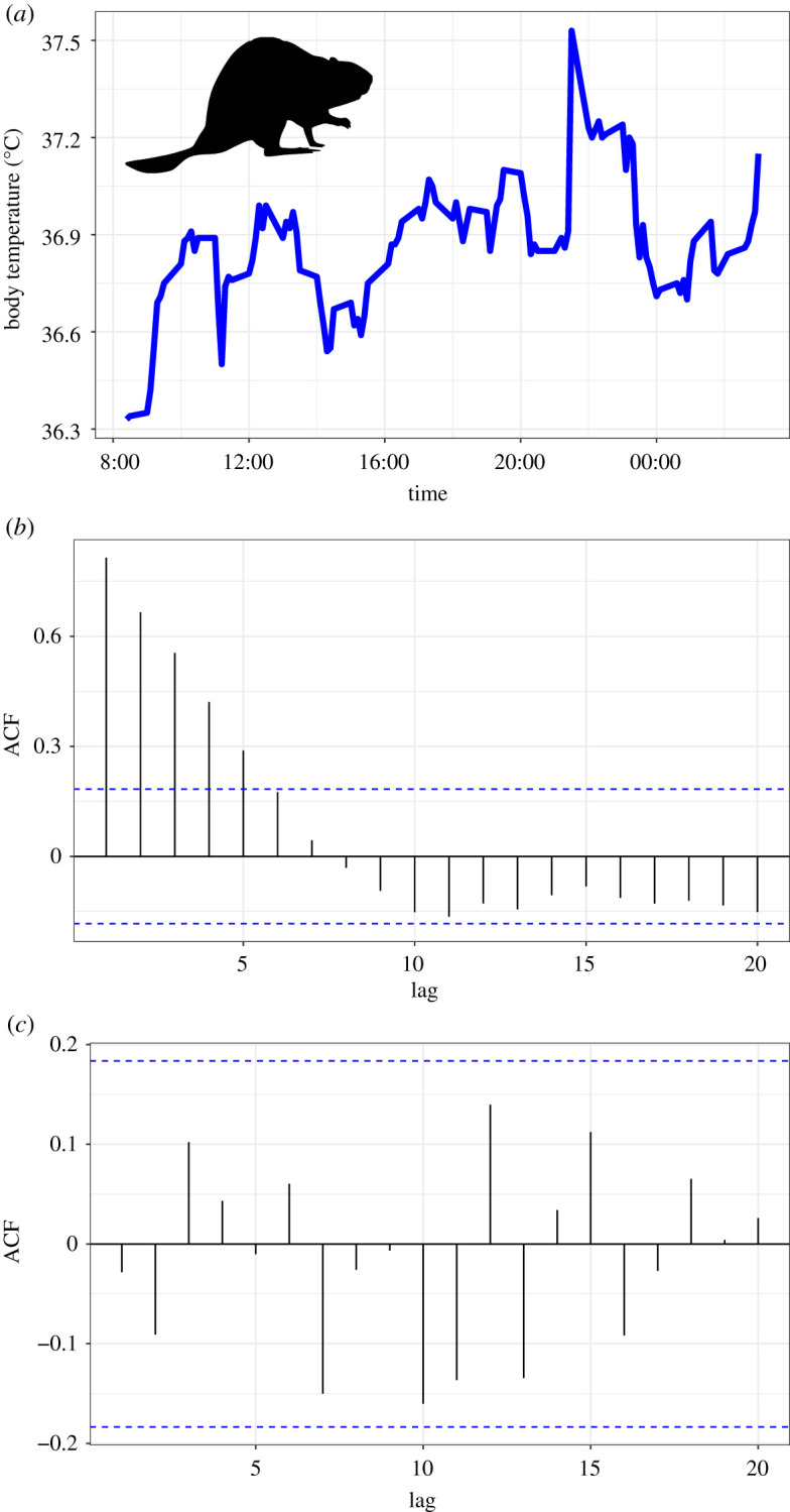
Time-series data and model output of a real physiological dataset on beaver body temperature. (a) Beaver body temperature data from a single individual recorded every 10 min over approximately 24 h. (b) Modelling these data using a GLS model with a basic AR(1) temporal autocorrelation structure produces notable issues, namely a value of phi (estimate of the correlation strength between consecutive measures/10 min time steps) of 0, when there is a clear serial dependence structure (a). Importantly, autocorrelation plots of the residuals as in (b) help us identify that there is still unmodelled autocorrelation in these data. (c) Applying a more complex temporal autocorrelation model (ARMA(2,0)) resolves these issues and produces non-zero estimates parameters such as phi, as well as satisfactory autocorrelation plots. This shows us that we cannot always assume fitting a model allowing for temporal autocorrelation automatically deals with the signal of temporal autocorrelation in the data. Always check your model diagnostics for these tell-tale signs that something is not as it should be.

(c) . Capturing the signal of autocorrelation

Once we have a candidate model fitted to our time-series data, there are two important things to check. First, pay close attention to the estimate of the correlation parameter (‘phi’ in the summary of a gls or lme fit). Values of 1 can indicate non-stationarity of the AR portion of the model, which is problematic, whereas values of 0 suggest you are not modelling the autocorrelation at all. Both suggest the model is a poor fit and that the model estimates should not be trusted. Second, inspect the plot of the autocorrelation function (ACF plots), an indication of the serial dependence between observations at different lags. The ACF plot for our AR(1) model of the beaver data still shows evidence of autocorrelation (figure 2b), while the phi parameter is 0. This means that we need something more sophisticated. Moving to an ARMA framework, and fitting an additional autoregressive parameter, i.e. an ARMA(2,0), the model appears to fix our autocorrelation (figure 2c), and we get non-zero estimates of phi. The key here is never to assume that fitting a model that can account for autocorrelation in your logger data, like and AR(1), means it will do so. I recommend the ‘ggtsdisplay’ function in the forecast package in R [52,53]; supplying it with residuals from the model will plot ACF, partial ACF and residuals-by-observation-order, all key diagnostic plots for adequacy of model fit [18].

(d) . Optimizing model selection

Knowing when a model is capturing the autocorrelation signal in the data is the first step, but how do we know (and evidence) that it is the best model for doing so? After all, we have a whole range of model specifications at our disposal; we can fit an arbitrary number of AR, MA or ARMA parameters. In the beaver example (figure 2), switching from AR(1) to ARMA(2,0) seemed to solve our problems, but may not be the optimal specification. As stated by Zuur et al. [40, p. 151], ‘the ARMA[p,q] can be seen as a black box to fix residual correlation problems', meaning we can experiment with different combinations of p and q parameters to be estimated in the data. Note that this entails a cost though: higher values of p and q can cause convergence problems because of the large amount of data needed to estimate them accurately [40], so there may be wisdom in restricting the set of models considered to be relatively small. We can use an information theoretic approach to select among candidate models to identify an optimal autocorrelation structure, using an information criterion such as Akaike's information criterion (AIC [58]). Be aware that the choice of information criterion (e.g. AIC versus Bayesian information criterion) can have an influence on which model is selected (i.e. has a lower information criterion score), depending on the signal in the data [18]. You unfortunately cannot use likelihood ratio tests to derive p-values for pairwise comparisons of these models because they are not nested. Next, we have to address how to optimize the fixed effects structure of the models, which adds a considerable degree of complexity (see below). I would argue it is sensible to optimize the autocorrelation structure first, and then use that model to test hypotheses about which variables are important, rather than test every combination of autocorrelation structure and possible fixed effect. Doing so would lead to unwieldy model sets and artificially increase levels of model selection uncertainty. When designing a candidate model set of autocorrelation structures to test, invoking the principles of parsimony by favouring the simplest structure that appears to adequately model the autocorrelation in your data (e.g. figure 2c) feels sensible. Information theory should help here, as it seeks to optimize the fit-complexity trade-off in our data and so should penalize models that are needlessly complex (i.e. contain unwarranted extra autocorrelation parameters). Again, be aware that different information criteria will penalize model complexities to different degrees, and so may yield divergent model sets [59].

How you then choose to optimize fixed effects structure requires further consideration. However, I would warn against using AIC to select among autocorrelation structures and then adopting a frequentist approach to perform variable selection among fixed effects. This will probably be seen as ‘mixing analysis paradigms' (see [60]). The same would be true of using Bayesian variable selection for fixed effects. Consequently, it feels as if we are canalized into the use of information theory throughout as the path of least resistance. Finally, one key thing to watch out for in these models is residual degrees of freedom. You will often be given a false impression of residual degrees of freedom because of the way sample size gets inflated by high recording rates of a logger. A 1000 record individual track with only a mean and slope estimated in the model does not yield 998 degrees of freedom, even if the model tells you it does, because the measurements are non-independent. This could have implications of Type I error rates [38,39], which we will investigate later on (see the ‘Controlling error rates to allow robust hypothesis testing’ section). Note that the use of information criteria obscures this problem [38] because model tables of metrics like AIC often only display number of estimated parameters, not assumed residual degrees of freedom.

(e) . Optimizing statistical power for biologging studies

Now that we have dealt with some of the key modelling approaches for physiological data, we should address perhaps the most important question of all. Before we have even deployed our first logger, how do we design a biologging study that is adequately powered to detect the effects we are interested in? Ecology textbooks will tell you it is reasonably straightforward to work this out [61]: (i) decide on a biologically meaningful effect size you want to detect, such as the mean difference in a trait between treatment groups; (ii) perform a power analysis to estimate the per-group sample size that gives you greater than 80% power to detect that difference; and (iii) design and execute the study using those sample size guidelines. However, in biologging studies, the relationship between devices deployed/implanted and devices retrieved is not so straightforward. Devices fail, or are lost, or sometimes are deployed without first being switched on. In the case of archival loggers, the need to catch the same individual twice introduces a degree of stochasticity that can challenge even the most elegant of power analyses. This does not mean you should dismiss the use of performing a power analysis before you deploy any loggers. In ethical terms, it might be important to know you are not deploying more loggers than necessary and causing undue harm (see [62–65]), or that you are not deploying loggers for a question you have no power to answer. In such cases then conducting a power analysis is sensible, but resources on how to do this for biologging studies are lacking.

To demonstrate the use of simulation and power analyses for informing biologging studies, we can examine hypothetical time-series depth data from fishes, where our central question is whether there is a difference in mean depth between the males and females (figure 3a). These data were generated from an AR(1) model with an assumed autocorrelation of 0.5, and an expected mean difference between males and females of 20 m. Running 1000 replicate simulations at each per-sex sample size from 5 to 50 in steps of 5 yields a power curve suggesting we would need data from at least 35 individuals of each sex to detect a difference of that magnitude reliably (figure 3b).

Figure 3.

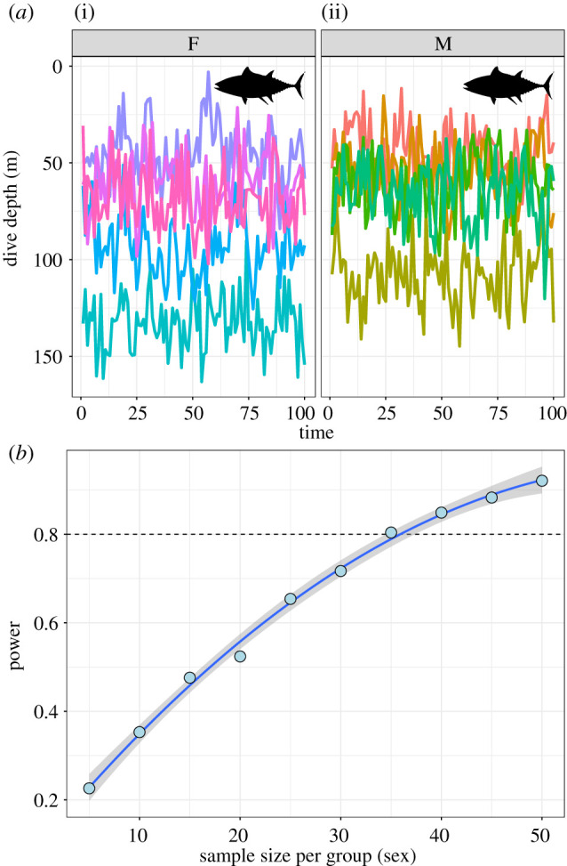
Power analyses for physiological biologging studies. (a) Example data from loggers recording time-series depth data of five female (i) and five male (ii) fish. Different coloured traces denote different individuals. The data-generating process assumed a 20 m difference in the average dive depth between sexes, with equal variance of each sex, and an AR(1) temporal autocorrelation structure in the data with rho = 0.5. (b) Power curve of sample size versus expected statistical power for detecting the differences in dive depth between males and females. The x-axis denotes increasing sample size per sex (x = 5 represents a total sample size of 10 deployed (and retrieved!) loggers). These data show that we would need at least 35 loggers per sex to reach the threshold of 80% power at the assumed effect size. A larger difference between the sexes in the mean dive depth would probably require fewer loggers to be deployed. The key here is to be aware of the smallest meaningful difference you wish to detect and to conduct power simulations using that effect size before deploying any loggers.

For our fish example, 35 individuals per sex might seem like a lot, but it is worth pointing out that in biologging studies, we have many additional sources of variance to incorporate into our power analysis over and above simply the within- versus among-sex variance in the trait of interest. Incorporating these sources of uncertainty is important to ensure your power estimates are reliable. If you have conducted a similar study previously, or have access to such a study or its raw data, some exploratory modelling will give you a good expectation of the complexity and shape of the data-generating process for your organism (e.g. AR(1) or ARMA(1,1) or ARMA(p,q)—How strong is the correlation between measures? How noisy is the time-series relationship?). All of these variables will affect your expected power to detect biological differences between the sexes, and so it might be prudent to use simulation to see how your assumptions change your threshold sample size for 80% power. You could even use it to understand how a certain rate of logger failure may affect downstream power, and you could use data from previous studies to estimate a realistic failure rate to include in power simulations. All the code for generating the data and power analysis in figure 3 is provided (see Data accessibility section), and so should provide a solid foundation for expanding to more complex cases for your own physiological data and studies.

(f) . Individual replication and random effects

Despite our best intentions, we might be left with a considerably smaller sample size than the number of devices we initially set out with, because some of those devices are still swimming or flying about out in the wild. In such situations, we need to know how to make the most of our data, part of which entails working out if we can trust our estimates from our models. Quantifying among-individual variance in a trait is often of principal interest to physiologists, or we might simply want to model that variation, so we can ‘ignore’ its effects on our key variables [37]. For our biologging data, this is equivalent to asking if individuals differ in a mean trait value of being measured, which we can achieve by fitting individual identification as a random intercept term in a mixed modelling framework (e.g. an lme or GAMM fit). Figure 4a shows some example data of body temperature of five shorebirds in flight. What we want to know is how sensitive our estimate of among-individual variation in the trait is to low sample size. For these data, the model was generated under an AR(1) process with phi = 0.5, a mean trait value of 40 (°C) and a standard deviation among individuals of 5. Note this may make the test fairly conservative, given how large a difference this is (figure 4a). By varying the sample size in steps of 2 from 2 to 20, we can investigate how parameter precision and accuracy change. The bad news is that low individual replication (less than 10 individual loggers retrieved) leads to poor accuracy and precision of the key metric of interest (figure 4b). Similar patterns are seen for our estimate of the strength of autocorrelation in the data (figure 4c), though it seems to be precision that suffers most here. Interestingly, this suggests that sample size requirements may be more stringent than for more ‘standard’ mixed models, where at least five levels of the random effect are usually required [37,43]. This is perhaps not too surprising, given that we are asking a lot more of the model in this instance, in that it has to account for serial dependence of data too. There is not much we can do here if we cannot alter the sample size. This means that when physiologging studies capture data from a limited number of animals, they must be aware that estimates have to be interpreted with caution, especially if a central question of the paper pertains to variation among individuals. This might be especially important for studies like our fish dive depth study (figure 3), where estimating among-individual variation accurately is critical to being able to detect the between-sex variation that forms the central question of the investigation. We have evidence here that low random effect replication compresses that estimate of among-individual differences, which can then compromise our statistical power.

Figure 4.

Effect of replication of random effects (number of individuals) on precision and accuracy of model estimates. (a) Time series of body temperature during flight for 10 individuals of a hypothetical shorebird species. Different colours represent different individuals. Data were generated using an AR(1) model with rho = 0.5 and the shape of the random effect distribution, representing true among-individual variation, had parameters μ = 40 and s.d. = 5. (b) Distribution of model estimates after 1000 replicate simulations for each value of individual sample size, ranging from 2 to 20. Different bar widths represent 66 and 95% intervals of the parameter distributions. At low individual/random effect replication (less than 10), both accuracy and precision of the estimate of among-individual variation are compromised (true s.d. value 5, dashed line). Above 10 ‘levels’ of the random effect, estimates stabilize in both accuracy and precision. The estimation accuracy of the autocorrelation parameter is uniform for all sample sizes on average, but precision suffered at values n < 8. Collectively, these data show that even if autocorrelation is being ‘dealt with’ by the models, the resulting parameter estimates may be quite unreliable if random effect sample sizes are low.

(g) . Controlling error rates to allow robust hypothesis testing

Along with variance components, it is important to understand how accurate parameter estimates of our fixed effects are, under conditions of both low sample size and incorrect model specification. There are two main quantities we are interested in knowing; the false-positive (Type I error) and false-negative (Type II error) rates. So, we will explore the incidence of these two types of error by modelling some more shorebird data similar to that in figure 4a. This time though, the data-generating model is more complex, being an ARMA(2,1) model (see https://github.com/xavharrison/Biologging for more details on the simulations). We assume the same degree of among-individual variation, and a true (known) effect of a change in the mean over time (β_TIME = 0.02). We also include in our dataset a nuisance parameter with no effect on the outcome, helpfully called ‘nuisance’ (β_NUISANCE = 0). For 1000 replicate simulations, I investigate the accuracy of these models assuming a sample size of 5 versus a sample size of 20 individuals, and when one fits an AR(1) versus ARMA(2,1) model. We have good reason to expect from the results in figure 4 that the models might struggle at the lower sample sizes, so I would predict that at n = 5 we will suffer increased Type I and Type II error rates. This would manifest as concluding nuisance was significant, and failing to conclude that time is significant, more often when n = 5. I would also predict that these issues will be worse when we use too simple a model to analyse the data (i.e. use an AR(1) model when an ARMA(p,q) might be more appropriate). For simplicity in these simulations, I consider something to be ‘significant’ when the model returns a non-zero estimate of β (for either time or nuisance) assessed using the Wald tests. So this is not the same as, for example, a likelihood ratio test between two models returning a significant p-value, though in reality these are likely to be correlated.

A key concern with any modelling approach is how accurate and precise the parameter estimates derived from our models are. Poorly specified models, and imprecise model estimates, can obscure our ability to test hypotheses about what variables are driving variation in our data. So first let us consider parameter accuracy, which is displayed in figure 5a. Just as for our simulations in figure 4, accuracy and precision of variance components are compromised at low sample sizes (top left panel, figure 5a). What is interesting here is that this problem is exacerbated when we use an improper model structure. We see similar trends in the estimates of phi in the models—the simplistic AR(1) model, being able to estimate only one of the two autocorrelation parameters, gets it wrong. But the degree of imprecision is not a function of sample size. With regard to statistical power, the results from our n = 20 models are encouraging (figure 5b). Our ARMA(2,1) model reliably estimates a non-zero coefficient of the slope for time greater than 80% of cases, and the Type I error rate for the nuisance variable is adequately controlled. Things are not so positive for the AR(1) models, where we lose the power to detect the time effect. This does not occur because the mean value is biased (figure 5a), but because the precision of the estimate is compromised, i.e. high uncertainty of effect size. Similar trends are seen for cases where n = 5 (figure 5c), where power for all effects is reduced.

Figure 5.

The effect of model structure and sample size on model accuracy. Data were generated using an ARMA(2,1) autocorrelation structure with sample size (number of individuals) of 5 or 20 and 100 values per time series. Model fitting used either a simple AR(1) or ARMA(2,1) correlation structure, i.e. the latter was the data-generating model. All models contained an effect of time (β = 0.02) and included a nuisance variable (nuisance) with no effect on the outcome (β = 0). (a) Parameter estimates after 1000 replicate simulations for each sample size and correlation structure. Only the first phi parameter of the ARMA model is shown for comparison with the AR model (equivalent to rho). (b,c) The distributions of rho values for the two fixed effects (nuisance and time) derived from the summary tables, i.e. based on Wald tests for n = 20 (b) and n = 5 (c). Note this is not a formal test of a variable's ‘significance’ through model selection, but gives a good indication of the model's assumed precision of the estimate.

So, there is some good news buried in here. With the cautionary note that these are a limited set of simulations for demonstration purposes, we do not seem to be at risk of increased Type I error either when sample sizes are small or when we use suboptimal model structures. This runs counter to expectation/predictions. What we can say is that we risk increased Type II errors under both conditions, missing out on recovering that potentially interesting effect of time. The good news is that although we cannot do anything about our final sample size, we can optimize model structure to ensure we recover stable and reliable estimates from our hard-won data. Though best practice recommendation is to use AIC to judge the relative fit of models with different autocorrelation structure fitted to the same data, the robustness of this approach is something that deserves to be empirically tested in future work.

(h) . Beyond simple autocorrelation structures

The models discussed so far are relatively simple, and may only form the foundation of data exploration before moving on to more complex analyses of physiological data. In many cases, simply modelling the autocorrelation process in our data, and how it may be influenced by individual traits such as sex (e.g. figure 4), may be insufficient. In recent years, and especially in the area of biologging focused on measuring animal accelerometry, both ML techniques [66] and HMM [67] have become popular approaches. For example, Bidder et al. [68] demonstrate how simple k-nearest neighbour ML algorithms can be used to classify behavioural states of multiple animal species with high accuracy and precision, including discrimination between dive, flight and walking states in cormorants. At the start of this article, we discussed the idea that we might want to use the raw data from loggers to generate summary statistics, e.g. count processes such as number of dives, or proportion metrics such as time spent foraging. Both ML and HMM provide the mechanism by which we calculate the frequencies of those behaviours, or proportion of time spent displaying them, that can then place us back in the realm of more familiar modelling techniques such as general(ized) linear (mixed effect) models (GLMs and GLMMs). HMM can also reveal more nuanced patterns in the data than dichotomous ‘doing the behaviour or not’ by classifying multiple variants/states of a given behaviour (e.g. dive behaviour in short-finned pilot whales [69]). It is worth noting that these tools are not just the preserve of movement ecologists. For example, Reby et al. [70] used HMMs to classify vocal structure and identify individual vocal signatures in red deer.

One potential issue with ML techniques is that they assume that measurements (i.e. logger data) are independent, whereas we know that they are likely to show strong serial dependence. HMM, as stochastic time-series models, can address this issue by explicitly modelling the serial dependence in the data [55,71]. HMMs can then be used in conjunction with environmental data, for example, to probe correlations between behavioural states and the external conditions experienced by the host [72]. In this work, I have demonstrated that even for simple time-series data, variation in model specification and replication of data can have marked consequences for model robustness and, therefore, any biological inference we may wish to make about the system. The same issues will be present, and important to consider, if we wish to skip the simpler models and dive straight into HMM approaches or similar. Quantitative assessments of how number of loggers deployed, and per-device data quality and quantity affect the accuracy and precision of HMM estimates should be prioritized to assure us we can trust the results of any hypothesis testing exercise in this study. Advances in biologging technology, and the species upon which they can be deployed, are occurring rapidly (see Williams et al., this issue [73]); ideally, we should continue to assess and refine the modelling framework designed to handle the outputs of those loggers simultaneously, to maximize the informativeness and use of biologging studies.

(i) . A simple workflow for tackling data analysis

Analysis of biologging data is complex, even before we have wandered into the realms of HMM and ML algorithms to classify behaviours (see [55]). Modelling time series from loggers presents some unique challenges for physiologists over and above the use of the ‘standard’ mixed model toolkit (table 1). The issues discussed in the paper, how they manifest in our data and potential solutions to deal with them are presented in table 2. These issues should hopefully provide a workflow of steps to go through when designing biologging studies. Clearly, the day can be won or lost before any loggers are even deployed, depending on how well designed the study is. Power analyses, though more complex than for traditional field experiments, can give us invaluable insights into the levels of replication needed to detect effects of interest, especially if one builds stochastic failure rates into the models. The power simulations and results in this paper provide a springboard from which to design your own power analysis simulations, or stress-test models. Through some exploratory simulations, we have seen that small sample sizes will compromise statistical power by driving up the incidence of Type II error rates. There is no easy fix for small sample sizes once you are at the modelling stage—we simply have to acknowledge that some of the model estimates, from variance components to fixed effect coefficients, will be unreliable and draw only very judicious conclusions about physiological data. But the key take-home message is that these effects can and should be minimized with thoughtful and careful application of modelling tools to find the optimal modelling structure. Time spent investigating fit improvements of more complex autocorrelation structures will be time well spent, as optimizing this element of models can have dramatic effects on Type II error rates. Increasingly more complex models (e.g. ARMA[p,q] structures) are increasingly more data-hungry, and can give rise to their own set of problems if you ask too much of them while feeding them too few data. But the same is also true of the more sophisticated modelling tools discussed here, such as HMMs.

Table 2.

Five key issues in the design of biologging studies and handling of resulting data, with potential solutions.

issue	outcome and diagnosis	potential solution
1. uncertainty over number of loggers to deploy in study to ensure adequate statistical power	lack of care over study design may mean compromised power to detect differences among treatment groups of interest	mine literature for effect sizes of interest in related species to inform power analysis. Be aware that choice of data-generating model may affect results: give careful attention to (i) the complexity of autocorrelation structure (e.g. AR(1) versus ARMA(2,1); (ii) amount of among-individual variation in the trait (the standard deviation of the random effects); and (iii) the amount of noise assumed (within-individual variation; ‘sigma’ in the time series). All will affect expected power
2. ignoring time-series structure in datasets by fitting GLMs or t-tests to data to test for differences between individuals or groups	inflated Type I error rates	use models that can deal with and quantify temporal autocorrelation in the data, e.g. generalized least squares (GLS), models fitted in nlme, and generalized additive (mixed) models [GA(M)Ms]
3. time-series models are too simple given complexity of data	poor model performance, e.g. estimates of phi in models collapse to 0, making model estimates potentially untrustworthy. ACF plots will still show the presence of autocorrelation	use more complex models e.g. ARMA(2,0) or ARMA(2,1) models. Select among models based on AIC, but inspect model estimates carefully. There is wisdom to fitting an autocorrelation function that is complex enough, but not more complex than it needs to be to avoid model convergence issues
4. once retrieved, very few individual tag IDs, or low replication of tracks for each logger	biased random effect estimates, though estimates of temporal autocorrelation relatively robust	interpret among-tag/among-individual variance from mixed models with caution
5. obtaining robust estimates of effect sizes for variables in models	incorrect model specification will lead to biased parameter estimates for some model components, especially autocorrelation parameters random effects (see also issues 3 and 4). Increased risk of Type II error for important variables, owing to increased s.e. of effect sizes. Limited evidence of increased Type I error for the same reason	fit multiple competing models with different autocorrelation structures and pay attention to parameter estimates. Are effect sizes non-significant because they are near zero, or because they have large standard errors? In the latter case, more suitable autocorrelation structures may improve the precision of estimates

Biologging datasets often appear immensely data-rich, containing thousands of data points, but inherent properties of those data such as serial autocorrelation reduce the information content of those data considerably. Indeed, the huge datasets can often obscure low individual replication (e.g. number of tags/devices), which can have significant impacts on the accuracy and/or precision of model estimates. Our ultimate goal is to test hypotheses about what drives variation in observed physiological state variables, but it is critical that we do not fit models to physiology data blindly assuming that they automatically produce robust tests of those hypotheses. As with all ecological modelling, models of physiological data should be as simple as they need to be, but no more so.

Data accessibility

All materials needed to reproduce the analyses and figures in this manuscript are provided as an R Markdown document on GitHub at https://github.com/xavharrison/Biologging.

Competing interests

I declare I have no competing interests.

Funding

I received no funding for this study.

References

- 1.Wilmers CC, Nickel B, Bryce CM, Smith JA, Wheat RE, Yovovich V. 2015. The golden age of bio-logging: how animal-borne sensors are advancing the frontiers of ecology. Ecology 96, 1741-1753. ( 10.1890/14-1401.1) [DOI] [PubMed] [Google Scholar]
- 2.Hawkes LA, Exeter O, Henderson SM, Kerry C, Kukuluya A, Rudd J, Whelan S, Yoder N, Witt MJ. 2020. Autonomous underwater videography and tracking of basking sharks. Anim. Biotelemetry 8, 29. ( 10.1186/s40317-020-00216-w) [DOI] [Google Scholar]
- 3.Smith BJ, Hart KM, Mazzotti FJ, Basille M, Romagosa CM. 2018. Evaluating GPS biologging technology for studying spatial ecology of large constricting snakes. Anim. Biotelemetry 6, 1. ( 10.1186/s40317-018-0145-3) [DOI] [Google Scholar]
- 4.Hawkes LA, et al. 2017. Do bar-headed geese train for high altitude flights? Integr. Comp. Biol. 57, 240-251. ( 10.1093/icb/icx068) [DOI] [PubMed] [Google Scholar]
- 5.Muller C, Childs AR, Duncan MI, Skeeles MR, James NC, van der Walt KA, Winkler AC, Potts WM. 2020. Implantation, orientation and validation of a commercially produced heart-rate logger for use in a perciform teleost fish. Conserv. Physiol. 8, coaa035. ( 10.1093/conphys/coaa035) [DOI] [PMC free article] [PubMed] [Google Scholar]
- 6.Brijs J, Sandblom E, Axelsson M, Sundell K, Sundh H, Kiessling A, Berg C, Gräns A. 2019. Remote physiological monitoring provides unique insights on the cardiovascular performance and stress responses of freely swimming rainbow trout in aquaculture. Sci. Rep. 9, 9090. ( 10.1038/s41598-019-45657-3) [DOI] [PMC free article] [PubMed] [Google Scholar]
- 7.Thompson D, Fedak MA. 1993. Cardiac responses of grey seals during diving at sea. J. Exp. Biol. 174, 139-164. ( 10.1242/jeb.174.1.139) [DOI] [PubMed] [Google Scholar]
- 8.Vyssotski AL, Serkov AN, Itskov PM, Dell'Omo G, Latanov AV, Wolfer DP, Lipp H-P. 2006. Miniature neurologgers for flying pigeons: multichannel EEG and action and field potentials in combination with GPS recording. J. Neurophysiol. 95, 1263-1273. ( 10.1152/jn.00879.2005) [DOI] [PubMed] [Google Scholar]
- 9.Hussey NE, et al. 2015. Aquatic animal telemetry: a panoramic window into the underwater world. Science 348, 1255642. ( 10.1126/science.1255642) [DOI] [PubMed] [Google Scholar]
- 10.Kays R, Crofoot MC, Jetz W, Wikelski M. 2015. Terrestrial animal tracking as an eye on life and planet. Science 348, aaa2478. ( 10.1126/science.aaa2478) [DOI] [PubMed] [Google Scholar]
- 11.Miyazawa Y, Kuwano-Yoshida A, Doi T, Nishikawa H, Narazaki T, Fukuoka T, Sato K. 2019. Temperature profiling measurements by sea turtles improve ocean state estimation in the Kuroshio-Oyashio Confluence region. Ocean Dyn. 69, 267-282. ( 10.1007/s10236-018-1238-5) [DOI] [Google Scholar]
- 12.Williams HJ, et al. 2017. Identification of animal movement patterns using tri-axial magnetometry. Move. Ecol. 5, 6. ( 10.1186/s40462-017-0097-x) [DOI] [PMC free article] [PubMed] [Google Scholar]
- 13.Harrison PM, Gutowsky LF, Martins EG, Patterson DA, Cooke SJ, Power M. 2016. Temporal plasticity in thermal-habitat selection of burbot Lota lota a diel-migrating winter-specialist. J. Fish Biol. 88, 2111-2129. ( 10.1111/jfb.12990) [DOI] [PubMed] [Google Scholar]
- 14.Chmura HE, Glass TW, Williams CT. 2018. Biologging physiological and ecological responses to climatic variation: new tools for the climate change era. Front. Ecol. Evol. 6, 92. ( 10.3389/fevo.2018.00092) [DOI] [Google Scholar]
- 15.Lewis KP, Vander Wal E, Fifield DA. 2018. Wildlife biology, big data, and reproducible research. Wildl. Soc. Bull. 42, 172-179. ( 10.1002/wsb.847) [DOI] [Google Scholar]
- 16.Bowlin MS, Wikelski MC, Cochran WW. 2004. The relationship between individual morphology, atmospheric conditions, and inter-individual variation in heart rate and wingbeat frequency during natural migration in the Swainsons thrush (Catharus ustulatus). Integr. Comp. Biol. 44, 529. [Google Scholar]
- 17.Kooyman GL. 1965. Techniques used in measuring diving capacities of Weddell seals. Polar Rec. (Gr. Brit.) 12, 391-394. ( 10.1017/S003224740005484X) [DOI] [Google Scholar]
- 18.Guerrier S, Molinari R, Xu H, Zhang Y. 2019. Applied time series analysis with R. See https://smac-group.github.io/ts/ (accessed 20 August 2020).
- 19.Bishop CM, et al. 2015. The roller coaster flight strategy of bar-headed geese conserves energy during Himalayan migrations. Science 347, 250-254. ( 10.1126/science.1258732) [DOI] [PubMed] [Google Scholar]
- 20.elmegaard SL, Johnson M, Madsen PT, McDonald BI. 2016. Cognitive control of heart rate in diving harbor porpoises. Curr. Biol. 26, R1175-R1176. ( 10.1016/j.cub.2016.10.020) [DOI] [PubMed] [Google Scholar]
- 21.Meisel C, Bailey K, Achermann P, Plenz D. 2017. Decline of long-range temporal correlations in the human brain during sustained wakefulness. Sci. Rep. 7, 11825. [DOI] [PMC free article] [PubMed] [Google Scholar]
- 22.Rattenborg NC, Voirin B, Cruz SM, Tisdale R, Dell'Omo G, Lipp HP, Wikelski M, Vyssotski AL. 2016. Evidence that birds sleep in mid-flight. Nat. Commun. 7, 1-9. ( 10.1038/ncomms12468) [DOI] [PMC free article] [PubMed] [Google Scholar]
- 23.Vyssotski AL, Dell'Omo G, Dell'Ariccia G, Abramchuk AN, Serkov AN, Latanov AV, Loizzo A, Wolfer DP, Lipp HP. 2009. EEG responses to visual landmarks in flying pigeons. Curr. Biol. 19, 1159-1166. ( 10.1016/j.cub.2009.05.070) [DOI] [PubMed] [Google Scholar]
- 24.Voirin B, Scriba MF, Martinez-Gonzalez D, Vyssotski AL, Wikelski M, Rattenborg NC. 2014. Ecology and neurophysiology of sleep in two wild sloth species. Sleep 37, 753-761. ( 10.5665/sleep.3584) [DOI] [PMC free article] [PubMed] [Google Scholar]
- 25.Parr N, Bishop CM, Batbayar N, Butler PJ, Chua B, Milsom WK, Scott GR, Hawkes LA. 2019. Tackling the Tibetan Plateau in a down suit: insights into thermoregulation by bar-headed geese during migration. J. Exp. Biol. 222, jeb203695. ( 10.1242/jeb.203695) [DOI] [PubMed] [Google Scholar]
- 26.Streicher S, Lutermann H, Bennett NC, Bertelsen MF, Mohammed OB, Manger PR, Scantlebury M, Ismael K, Alagaili AN. 2017. Living on the edge: daily, seasonal and annual body temperature patterns of Arabian oryx in Saudi Arabia. PLoS ONE 12, e0180269. ( 10.1371/journal.pone.0180269) [DOI] [PMC free article] [PubMed] [Google Scholar]
- 27.Hume T, Geiser F, Currie SE, Körtner G, Stawski C. 2020. Responding to the weather: energy budgeting by a small mammal in the wild. Cur. Zool. 66, 15-20. ( 10.1093/cz/zoz023) [DOI] [PMC free article] [PubMed] [Google Scholar]
- 28.Meir JU, Champagne CD, Costa DP, Williams CL, Ponganis PJ. 2009. Extreme hypoxemic tolerance and blood oxygen depletion in diving elephant seals. Am. J. Physiol. Regul. Integr. Comp. Physiol. 297, R927-R939. ( 10.1152/ajpregu.00247.2009) [DOI] [PubMed] [Google Scholar]
- 29.Stockard TK, Heil J, Meir JU, Sato K, Ponganis KV, Ponganis PJ. 2005. Air sac PO2 and oxygen depletion during dives of emperor penguins. J. Exp. Biol. 208, 2973-2980. ( 10.1242/jeb.01687) [DOI] [PubMed] [Google Scholar]
- 30.Williams CL, Hicks JW. 2016. Continuous arterial PO2 profiles in unrestrained, undisturbed aquatic turtles during routine behaviors. J. Exp. Biol. 219, 3616-3625. ( 10.1242/jeb.141010) [DOI] [PMC free article] [PubMed] [Google Scholar]
- 31.Whitney NM, White CF, Smith BJ, Cherkiss MS, Mazzotti FJ, Hart KM. 2021. Accelerometry to study fine-scale activity of invasive Burmese pythons (Python bivittatus) in the wild. Anim. Biotelemetry 9, 1-3. ( 10.1186/s40317-020-00227-7) [DOI] [Google Scholar]
- 32.Van Walsum TA, Perna A, Bishop CM, Murn CP, Collins PM, Wilson RP, Halsey LG. 2020. Exploring the relationship between flapping behaviour and accelerometer signal during ascending flight, and a new approach to calibration. Ibis 162, 13-26. ( 10.1111/ibi.12710) [DOI] [Google Scholar]
- 33.Fehlmann G, O'Riain MJ, Hopkins PW, O'Sullivan J, Holton MD, Shepard EL, King AJ. 2017. Identification of behaviours from accelerometer data in a wild social primate. Anim. Biotelemetry 5, 1. ( 10.1186/s40317-017-0121-3) [DOI] [Google Scholar]
- 34.Meir JU, Robinson PW, Vilchis LI, Kooyman GL, Costa DP, Ponganis PJ. 2013. Blood oxygen depletion is independent of dive function in a deep diving vertebrate, the northern elephant seal. PLoS ONE 8, e83248. ( 10.1371/journal.pone.0083248) [DOI] [PMC free article] [PubMed] [Google Scholar]
- 35.Brown EN, Czeisler CA. 1992. The statistical analysis of circadian phase and amplitude in constant-routine core-temperature data. J. Biol. Rhythms 7, 177-202. ( 10.1177/074873049200700301) [DOI] [PubMed] [Google Scholar]
- 36.Sunagawa GA, Takahashi M. 2016. Hypometabolism during daily torpor in mice is dominated by reduction in the sensitivity of the thermoregulatory system. Sci. Rep. 6, 37011. ( 10.1038/srep37011) [DOI] [PMC free article] [PubMed] [Google Scholar]
- 37.Harrison XA, Donaldson L, Correa-Cano ME, Evans J, Fisher DN, Goodwin CE, Robinson BS, Hodgson DJ, Inger R. 2018. A brief introduction to mixed effects modelling and multi-model inference in ecology. PeerJ 6, e4794. ( 10.7717/peerj.4794) [DOI] [PMC free article] [PubMed] [Google Scholar]
- 38.Silk MJ, Harrison XA, Hodgson DJ. 2020. Perils and pitfalls of mixed-effects regression models in biology. PeerJ 8, e9522. ( 10.7717/peerj.9522) [DOI] [Google Scholar]
- 39.Arnqvist G. 2020. Mixed models offer no freedom from degrees of freedom. Trends Ecol. Evol. 35, 329-335. ( 10.1016/j.tree.2019.12.004) [DOI] [PubMed] [Google Scholar]
- 40.Zuur A, Ieno EN, Walker N, Saveliev AA, Smith GM. 2009. Mixed effects models and extensions in ecology with R. New York, NY: Springer. [Google Scholar]
- 41.Williams HJ, et al. 2020. Optimizing the use of biologgers for movement ecology research. J. Anim. Ecol. 89, 186-206. ( 10.1111/1365-2656.13094) [DOI] [PMC free article] [PubMed] [Google Scholar]
- 42.Schielzeth H, et al. 2020. Robustness of linear mixed-effects models to violations of distributional assumptions. Methods Ecol. Evol. 11, 1141-1152. ( 10.1111/2041-210X.13434) [DOI] [Google Scholar]
- 43.Harrison XA. 2015. A comparison of observation-level random effect and beta-binomial models for modelling overdispersion in binomial data in ecology & evolution. PeerJ 3, e1114. ( 10.7717/peerj.1114) [DOI] [PMC free article] [PubMed] [Google Scholar]
- 44.R Core Team. 2020. R: a language and environment for statistical computing. Vienna, Austria: R Foundation for Statistical Computing. See https://www.R-project.org/. [Google Scholar]
- 45.Kay M. 2020. tidybayes: tidy data and geoms for Bayesian models. R package version 2.1.1.9000. See http://mjskay.github.io/tidybayes/. ( 10.5281/zenodo.1308151) [DOI]
- 46.Wickham H. 2016. Ggplot2: elegant graphics for data analysis. New York, NY: Springer-Verlag. See https://ggplot2.tidyverse.org. [Google Scholar]
- 47.Wickham H, François R, Henry L, Müller K. 2020. dplyr: a grammar of data manipulation. R package version 0.8.5. See https://CRAN.R-project.org/package=dplyr.
- 48.Wilke C. 2019. cowplot: streamlined plot theme and plot annotations for 'ggplot2'. R package version 1.0.0. See https://CRAN.R-project.org/package=cowplot.
- 49.Pinheiro J, Bates D, DebRoy S, Sarkar D, Core Team R. 2020. nlme: linear and nonlinear mixed effects models. R package version 3.1-147. See https://CRAN.R-project.org/package=nlme.
- 50.Guerrier S, Balamuta J, Molinari R, Lee J, Zhang Y. 2019. simts: time series analysis tools. R package version 0.1.1. See https://CRAN.R-project.org/package=simts.
- 51.Chamberlain S. 2020. rphylopic: get 'silhouettes' of 'organisms’ from 'Phylopic'. R package version 0.3.0. See https://CRAN.R-project.org/package=rphylopic.
- 52.Hyndman R, et al. 2020. forecast: forecasting functions for time series and linear models. R package version 8.12. See http://pkg.robjhyndman.com/forecast.
- 53.Hyndman RJ, Khandakar Y. 2008. Automatic time series forecasting: the forecast package for R. J. Stat. Softw. 26, 1-22.19777145 [Google Scholar]
- 54.Andrews RD, Jones DR, Williams JD, Thorson PH, Oliver GW, Costa DP, Le Boeuf BJ. 1997. Heart rates of northern elephant seals diving at sea and resting on the beach. J. Exp. Biol. 200, 2083-2095. ( 10.1242/jeb.200.15.2083) [DOI] [PubMed] [Google Scholar]
- 55.Leos-Barajas V, Photopoulou T, Langrock R, Patterson TA, Watanabe YY, Murgatroyd M, Papastamatiou YP. 2017. Analysis of animal accelerometer data using hidden Markov models. Methods Ecol. Evol. 8, 161-173. ( 10.1111/2041-210X.12657) [DOI] [Google Scholar]
- 56.Zuur AF, Ieno EN, Elphick CS. 2010. A protocol for data exploration to avoid common statistical problems. Methods Ecol. Evol. 1, 3-14. ( 10.1111/j.2041-210X.2009.00001.x) [DOI] [Google Scholar]
- 57.Reynolds PS. 1994. Time-series analyses of beaver body temperatures. Chapter 11. In Case studies in biometry (eds Lange N, Ryan L, Billard L, Brillinger D, Conquest L, Greenhouse J), pp. 211-218. New York, NY: John Wiley and Sons. [Google Scholar]
- 58.Akaike H. 1974. A new look at the statistical model identification. IEEE Trans. Autom. Control 19, 716-723. ( 10.1109/TAC.1974.1100705) [DOI] [Google Scholar]
- 59.Brewer MJ, Butler A, Cooksley SL. 2016. The relative performance of AIC, AICC and BIC in the presence of unobserved heterogeneity. Methods Ecol. Evol. 7, 679-692. ( 10.1111/2041-210X.12541) [DOI] [Google Scholar]
- 60.Burnham KP, Anderson DR, Huyvaert KP. 2011. AIC model selection and multimodel inference in behavioral ecology: some background, observations, and comparisons. Behav. Ecol. Sociobiol. 65, 23-35. ( 10.1007/s00265-010-1029-6) [DOI] [Google Scholar]
- 61.Quinn GP, Keough MJ. 2002. Experimental design and data analysis for biologists. Cambridge, UK: Cambridge University Press. [Google Scholar]
- 62.Bodey TW, Cleasby IR, Bell F, Parr N, Schultz A, Votier SC, Bearhop S. 2017. A phylogenetically controlled meta-analysis of biologging device effects on birds: deleterious effects and a call for more standardized reporting of study data. Methods Ecol. Evol. 9, 946-955. ( 10.1111/2041-210X.12934) [DOI] [Google Scholar]
- 63.Portugal SJ, White CR. 2018. Miniaturization of biologgers is not alleviating the 5% rule. Methods Ecol. Evol. 9, 1662-1666. ( 10.1111/2041-210X.13013) [DOI] [Google Scholar]
- 64.Authier M, Péron C, Mante A, Vidal P, Grémillet D. 2013. Designing observational biologging studies to assess the causal effect of instrumentation. Methods Ecol. Evol. 4, 802-810. ( 10.1111/2041-210X.12075) [DOI] [Google Scholar]
- 65.Brlík V, et al. 2020. Weak effects of geolocators on small birds: a meta-analysis controlled for phylogeny and publication bias. J. Anim. Ecol. 89, 207-220. ( 10.1111/1365-2656.12962) [DOI] [PubMed] [Google Scholar]
- 66.Wang G. 2019. Machine learning for inferring animal behavior from location and movement data. Ecol. Inform. 49, 69-76. ( 10.1016/j.ecoinf.2018.12.002) [DOI] [Google Scholar]
- 67.McClintock BT, Langrock R, Gimenez O, Cam E, Borchers DL, Glennie R, Patterson TA. 2020. Uncovering ecological state dynamics with hidden Markov models. Ecol. Lett. 23, 1878-1903. ( 10.1111/ele.13610) [DOI] [PMC free article] [PubMed] [Google Scholar]
- 68.Bidder OR, Campbell HA, Gómez-Laich A, Urgé P, Walker J, Cai Y, Gao L, Quintana F, Wilson RP. 2014. Love thy neighbour: automatic animal behavioural classification of acceleration data using the k-nearest neighbour algorithm. PLoS ONE 9, e88609. ( 10.1371/journal.pone.0088609) [DOI] [PMC free article] [PubMed] [Google Scholar]
- 69.Quick NJ, Isojunno S, Sadykova D, Bowers M, Nowacek DP, Read AJ. 2017. Hidden Markov models reveal complexity in the diving behaviour of short-finned pilot whales. Sci. Rep. 7, 1-2. ( 10.1038/srep45765) [DOI] [PMC free article] [PubMed] [Google Scholar]
- 70.Reby D, André-Obrecht R, Galinier A, Farinas J, Cargnelutti B. 2006. Cepstral coefficients and hidden Markov models reveal idiosyncratic voice characteristics in red deer (Cervus elaphus) stags. J. Acoust. Soc. Am. 120, 4080-4089. ( 10.1121/1.2358006) [DOI] [PubMed] [Google Scholar]
- 71.Carter MI, McClintock BT, Embling CB, Bennett KA, Thompson D, Russell DJ. 2020. From pup to predator: generalized hidden Markov models reveal rapid development of movement strategies in a naïve long-lived vertebrate. Oikos 129, 630-642. ( 10.1111/oik.06853) [DOI] [Google Scholar]
- 72.Patterson TA, Basson M, Bravington MV, Gunn JS. 2009. Classifying movement behaviour in relation to environmental conditions using hidden Markov models. J. Anim. Ecol. 78, 1113-1123. ( 10.1111/j.1365-2656.2009.01583.x) [DOI] [PubMed] [Google Scholar]
- 73.Williams HJ, Shipley JR, Rutz C, Wikelski M, Wilkes M, Hawkes LA. 2021. Future trends in measuring physiology in free-living animals. Phil. Trans. R. Soc. B 376, 20200230. ( 10.1098/rstb.2020.0230) [DOI] [PMC free article] [PubMed] [Google Scholar]
Associated Data
This section collects any data citations, data availability statements, or supplementary materials included in this article.
Data Availability Statement