

Abstract
This article synthesizes two GIS-based accessibility measures into one framework, and applies the methods to examining spatial accessibility to primary healthcare in the Chicago 10-county region. The floating catchment area method defines the service area of physicians by a threshold travel time while accounting for the availability of physicians by their surrounded demands. The gravity-based method considers a nearby physician more accessible than a remote one and discounts a physician’s availability by a gravity-based potential. The former is a special case of the latter. Based on the 2000 Census and primary care physician data, this research assesses the variation of spatial accessibility to primary care in the Chicago region, and analyzes the sensitivity of results by experimenting with ranges of threshold travel times in the floating catchment area method and travel friction coefficients in the gravity model. The methods may be used to help the U.S. Department of Health and Human Services and state Health Departments improve health professional shortage areas designation.
Keywords: accessibility measures, two-step floating catchment area method, gravity model, GIS, healthcare access, physician shortage areas
Introduction
Accessibility refers to the relative ease by which the locations of activities, such as work, shopping and healthcare, can be reached from a given location (Bureau of Transportation Statistics or BTS, 1997, p.173). Access to healthcare varies across space because access to healthcare is affected by where health professionals locate (supply) and where people reside (demand) and neither health professionals nor population is uniformly distributed. Physician shortage has been especially pronounced in rural areas and impoverished urban communities (Council on Graduate Medical Education or COGME, 2000; Rosenblatt and Lishner, 1991). The U.S. federal government spends about $1 billion a year on programs designed to alleviate access problems, including awarding financial assistance to providers and assigning National Health Service Corps personnel to serve designated shortage areas (General Accounting Office or GAO, 1995). Any effective remedies begin with reliable measures of accessibility to healthcare.
Access to health care may be classified according to two dichotomous dimensions (potential vs. revealed and spatial vs. aspatial) into four categories such as: potential spatial access, potential aspatial access, revealed spatial access, and revealed aspatial access (Khan, 1992). Revealed accessibility focuses on actual use of health care services, whereas potential accessibility signifies the probable entry into the health care system, but does not ensure the automatic utilization of the offered services (Joseph and Phillips, 1984; Phillips, 1990; Thouez et al., 1988; Khan, 1992). Spatial access emphasizes the importance of spatial/distance variable (as a barrier or a facilitator), whereas the aspatial access stresses non-geographic barriers or facilitators such as social class, income, ethnicity, age, sex, etc. (Joseph and Phillips, 1984; Khan, 1992; Meade and Earickson, 2000, p.383–392). This paper focuses primarily on measuring potential spatial accessibility. The measures of potential spatial accessibility include regional availability and regional accessibility (Joseph and Phillips, 1984). The regional availability approach is simpler and measures distribution of supply versus demand within a region, often expressed as a population to practitioner ratio (or its variation) within that region. The regional accessibility approach considers such potential for complex interaction between supply and demand located in different regions and thus is more complex and requires more data (Joseph and Phillips, 1984).
The U.S. Department of Health and Human Services (DHHS) uses two main systems for identifying shortage areas (GAO, 1995; Lee, 1991). One designates Health Professional Shortage Areas (HPSA), the other Medically Underserved Areas or Populations (MUA/MUP). Both systems use the population to full-time-equivalent (FTE) primary care physician ratio within a “rational service area” as a basic indicator (e.g., 3,500:1 in HPSA designations), and thus are primarily regional availability measures of potential spatial access with some aspatial elements. For example, the HPSAs can include population groups (e.g., low-income or minority groups) and MUA/MUP considers aspatial factors such as infant mortality rate, income level and age. A rational service area may be (a) a whole county or groups of contiguous counties, (b) a portion of a county, or an area made up of portions of more than one county, or (c) established neighborhoods and communities. For details, see guidelines at http://bphc.hrsa.gov/dsd (last accessed December 3, 2002). This paper will focus on spatial factors. Our ongoing research will address aspatial issues, and results will be reported in the near future.
The problems of the regional availability measures are that (1) they can not reveal the detailed spatial variations within those large rational service areas (such as counties or group of counties) and (2) they carry the assumption that the boundaries are impermeable, i.e., the actual interaction across boundaries is not adequately accounted for (Joseph and Phillips, 1984). In other words, access to healthcare depends, not only upon the supply of resources in a community, but also the supply of such resources in neighboring communities (Wing and Reynolds, 1988; GAO, 1995) and the distance and ease of travel among them (Klienman and Makuc, 1983, p. 543). The severity of the two problems also changes with the scale (i.e., level of aggregation). The higher the aggregation level of rational service areas (i.e., the larger the areal unit), the more serious the internal variation problem is, but the less serious the permeability problem is. The reverse is true for lower aggregation level. The two cannot be easily reconciled within the framework of regional availability measures.
Recent revisions of criteria for designating HPSAs and MUAs/MUPs intend to address the problems by (1) using geographic units smaller than counties as “rational service areas” (e.g., minor civil divisions, census tracts), and (2) considering the impact of neighboring areas. For example, the third criterion in defining HPSAs specifies that medical resources in contiguous areas need to be “overutilized, excessively distant,or inaccessible”. Implementing this criterion requires incorporating regional accessibility measures. In other words, it calls for an integration of regional availability (demand to supply ratio) and regional accessibility (interaction between demand and supply) measures.
The increasing abundance of digital data (e.g., population data, street and road network, physician database) and advancement of GIS technology now make it possible to identify distributions of physicians and population at finer spatial resolutions (Mukuc et al., 1991; Love and Lindquist, 1995; Kohli et al., 1995; Parker and Campbell, 1998; Cromley and McLafferty, 2002; Lovett et al., 2002). In the meantime, the literature of accessibility measures has grown in a variety of fields (see related reviews in the following sections where methods are discussed). Several methods consider the effects of neighboring communities while accounting for availability of healthcare providers. Among others, the following two are most noticeable:
the spatial decomposition method by Radke and Mu (2000), and
the gravity-based method by Weibull (1976) and applied to healthcare access by Joseph and Bantock (1982).
This paper builds upon prior research, and makes contributions in the following ways:
It proves that the spatial decomposition method (referred to as the “two-step floating catchment area method” in this paper for reasons explained in a later section) is merely a special case of the gravity-based method, and thus synthesizes them into one framework. This reinforces the rationale of the two methods, which capture the same essence of accessibility measures.
Unlike most of prior work using straight-line distances, this research uses travel times to measure the spatial barrier between residents and physicians. In addition, the travel times are estimated systematically and consistently in a GIS environment, which have been either approximated by distances or estimated manually on a case by case basis (unpublished DHHS training manual).
The methods are applied to measuring healthcare accessibility using smaller geographic units (i.e., physicians in ZIP code areas and population in census tracts), and therefore more details of accessibility variations can be revealed.
Specifically, this paper examines spatial accessibility to primary healthcare in the Chicago 10-county region in 2000, with a focus on methodology issues. Results may be used to help the U.S. Department of Health and Human Services and state Health Departments for designing a better system for physician shortage area designation.
The Study Area, Data Sources and Travel Time Estimation
The 10 Illinois counties in the Chicago CMSA (Consolidated Metropolitan Statistical Area) are chosen as the study area for this paper. See Figure 1. The area represents a small portion of the state of Illinois (to be studied in a larger project) so that local variations may be displayed in reasonable details, yet this densely populated area accounts for two-thirds of population in Illinois in 2000. Both urban and rural areas are represented in the region since some peripheral counties are mostly rural. In order to account for “edge effects”, a 15-mile buffer zone (approximately 30 minutes travel time) is identified near the borders of the study area (except for the shorelines of Lake Michigan on the east). Accessibility measures in this buffer zone needs to be interpreted with caution because residents may seek healthcare outside of the study area.
Figure 1.
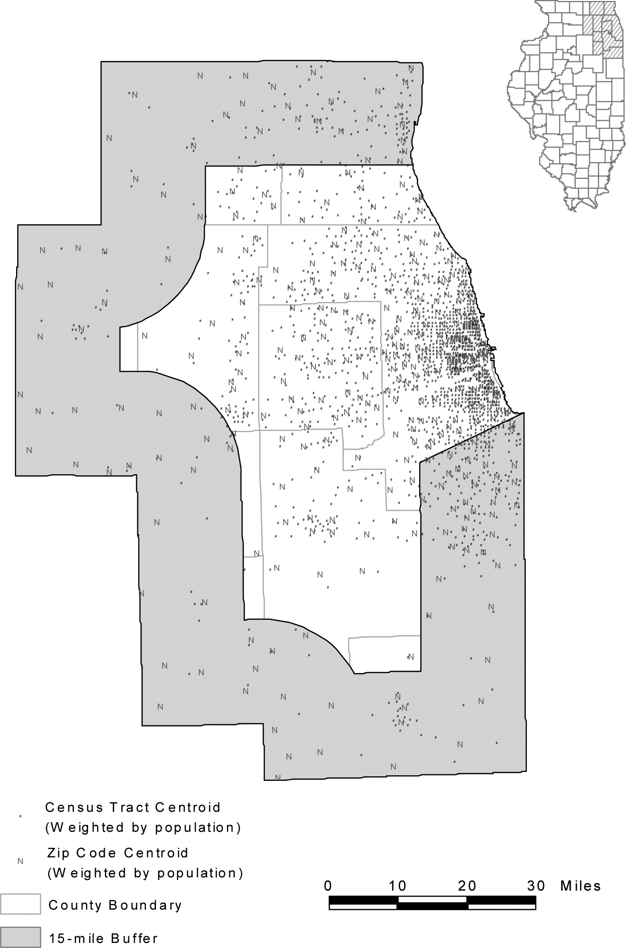
The Chicago 10-county region.
The population data were extracted from the 2000 Census Summary File 1 (U.S. Bureau of Census, 2001a), and the corresponding spatial coverages of census tracts and blocks were generated from the 2000 Census TIGER/Line files (U.S. Bureau of Census, 2001b). Since the population is seldom distributed homogeneously within a census tract, the population-weighted centroid instead of the simple geographic centroid of a census tract represents the location of population more accurately (Hwang and Rollow, 2000). A tract’s population centroid may be distant from its geographic centroid particularly in rural or peripheral suburban areas where tracts are large and population tends to concentrate in limited space. Weighted centroids are computed based on block-level population data such as:
| (1) |
| (2) |
where xc and yc are the x and y coordinates of the weighted centroid of a census tract, respectively; xi and yi are the x and y coordinates of the ith block centroid within that census tract, respectively; pi is the population at the ith census block within that census tract; and nc is the total number of blocks within that census tract. Census tract is chosen as the analysis unit for population distribution, since it is the lowest areal unit used in the current practice of shortage area designation, and the number of tracts is computationally manageable for travel time estimation and accessibility modeling. In the study area, there were 1,901 census tracts with a total population of 8,376,604 in 2000 (see Figure 1).
The primary care physician data of Illinois in 2000 were purchased from the Physician Master File of the American Medical Association (AMA) via Medical Marketing Service Inc. Primary care physicians include family physicians, general practitioners, general internists, general pediatricians, and some obstetrician-gynecologists (Cooper, 1994). This case study focuses on primary care physicians because these physicians are an integral component of a rational and efficient health delivery system and they are critical for the success of preventive care (Lee, 1995). Most of the HPSAs designated by the U.S. Department of Health and Human Services are also for primary medical cares (others are mental health and dental HPSAs). The methodology presented here can be easily adapted to identify shortage areas of other health care specialties, and at state and national levels.
Ideally, the physician locations should be geocoded by their street addresses with GIS software, a process of converting the address information to x and y coordinates of a point on the map by matching address name and interpolating the address range to those stored in a digital map (e.g., TIGER/Line file). However, a significant number of records in the Physician Master File only have “P. O. Box” addresses, which are not feasible for geocoding. This study simply used the centroid of zip code of a physician’s office address to represent the physician’s location. Only when the office addresses were not available, the zip codes of preferred addresses were used (such cases account for 18.5% of the records, which may or may not be office addresses). As physicians often choose to practice at populated places, population-weighted centroids instead of the simple geographic centroids of zip code areas were used, and computed similarly to census tract centroids as in equations (1) and (2). The population of each block whose centroid falls within a ZIP code area was used as weight to calculate the population-weighted centroid for that ZIP code. We are aware of the problems associated with using zip code data because zip codes may be totally unrelated to health care or demographic data. For example, some “point zips” are for small rural post offices that have only a set of boxes for mail pickup. Many in urban areas are for office building or government subdivisions that are unrelated to either physician or potential patients (Wing and Reynolds, 1988). However, zip code represents a finer resolution than county and has been used extensively in health research (e.g., Ng et al., 1993; Parker and Campbell, 1998; Knapp and Harwick, 2000). The AMA physician data do not identify how much percent of time each physician serves at one location among multiple offices, and thus do not enable us to obtain the number of full-time-equivalent (FTE) physicians. Converting to FTE physicians requires extensive surveys and field work (personal communication with Mary Ring and Jerry Partlow, Center for Rural Health, Illinois Department of Public Health, August 22, 2002), which are beyond the scope of this project. The focus of the paper is to demonstrate the methodology. Better physician information will certainly improve the result. There were 325 zip codes with 19,202 primary physicians in the study area in 2000 (see Figure 1). Table 1A in the Appendix also provides total numbers of primary care physicians and population, and their ratios in all 10 counties in the study area.
The methods of accessibility measures discussed in the next two sections utilize travel time between any pair of population and physician locations. Road networks for travel time estimation were also extracted from the 2000 Census TIGER/Line files. Assuming people taking the fastest path, we used the Arc/Info network analysis module to derive the shortest travel time between any two locations. Travel speeds may also be dictated by traffic signals and pre-set speed limits (often reduced in business districts or high residential density areas, see Illinois Department of Transportation or IDOT, 1977). For planning purposes, people can be assumed to travel at the speed limit, which is used as the impedance value for each road segment in the network quickest path computation. After a careful examination of the speed limit maps maintained by the Illinois Department of Transportation1, we developed several rules to approximate travel speeds based on the population density pattern (see Table A2 and Figure 1A in the Appendix). See Wang (2003) for more details of estimating travel times.
The Evolvement of Floating Catchment Area Methods
Given the broad interests in accessibility measures, several approaches have been developed in various applications. Earlier versions of the floating catchment area (FCA) method were used in assessing job accessibility (e.g., Peng, 1997; Wang, 2000). This method somewhat resembles to kernel estimation (e.g., Bailey and Gatrell, 1995), in which a “window” (kernel) is moved across a study area, and the density of events within the window is used to represent the density at the window’s center. In estimating the density, one may use a gravity model to weight events by the inverse of distances from the center. Figure 2 uses an example to illustrate the method. For simplicity, assume that each census tract has only one person residing at its centroid and each physician location has only one physician practicing there. Also assume that a threshold travel distance for primary health care is 15 miles. A 15-mile circle around the centroid of residential location 2 defines its catchment area (Peng, 1997 used a square to define a catchment area). Accessibility in a census tract is defined as the physician to population ratio within its catchment area. For instance, there are one physician (i.e., a) and eight residents within the catchment area, and thus accessibility to physicians in tract 2 is their ratio 1/8. The circle floats from one centroid to another while its radius remains the same. Similarly, there are two physicians (a and b) and five residents within the 15-mile catchment area of tract 3, and thus the accessibility in tract 3 is their ratio 2/5. The underlying assumption is that services that fall within the catchment area will be fully available to residents within that catchment area. This assumption is obviously faulty. For example, the distance between a physician and a resident within the catchment area may exceed the threshold travel time (e.g., distance between 1 and b is greater than the radius of the catchment of tract 3 in Figure 2). Furthermore, the physician at b is within the catchment of tract 3, but may not be fully available to serve residents within the catchment because he or she will also serve nearby (but outside the catchment) residents at 5, 8 or 11. Wang and Minor (2002) used travel times instead of straight-line distances to define the catchment area, but the fallacy remains.
Figure 2.

An earlier version of the floating catchment area (FCA) method.
In addressing the issues, Radke and Mu (2000) developed the “spatial decomposition method” to measure access to social services. The method computes the ratio of suppliers to residents within a service area centered at a supplier’s location and sums up the ratios for residents living in areas where different providers’ services overlap. Like the earlier versions of floating catchment area (FCA) approach, they used straight-line distances. In their study, analysis areas may be split by an overlaying circle, and service areas are a set of decomposed areas. In this research, we use centroids to represent whole census tracts or zip code areas for simplicity, and thus the process does not involve decomposition of polygons as described in Radke and Mu (2000). The method is referred to hereafter as the “two-step floating catchment area (FCA) method” to reflect its connection to the tradition of floating catchment area methods. The method uses travel times, and is implemented in two steps. The following procedures are organized in a way for easy interpretation using notation consistent with the gravity-based method to be introduced in the next section.
-
For each physician location j, search all population locations (k) that are within a threshold travel time (d0) from location j (i.e., catchment area j), and compute the physician to population ratio Rj within the catchment area:
(3) where Pk is the population of tract k whose centroid falls within the catchment (i.e., dkj≤d0), Sj is the number of physicians at location j, and dkj is the travel time between k and j.
For each population location i, search all physician locations (j) that are within the threshold travel time (d0) from location i (i.e., catchment area i), and sum up the physician to population ratios Rj at these locations:
| (4) |
In equ. (4), represents the accessibility at resident location i based on the two-step FCA method, Rj is the physician to population ratio at physician location j whose centroid falls within the catchment centered at i (i.e., dij≤d0), and dij is the travel time between i and j. A larger value of indicates a better accessibility at a location. The first step above corresponds to the assigning of an initial ratio to each service area centered at physician locations, and the second step corresponds to summing up the initial ratios in the overlapped service areas (where residents have access to multiple physician locations). This is similar, in effect, to decomposing the floating catchment area in Radke and Mu (2000). In implementation, a matrix of travel times between any pair of physician location and population location (dij or dkj) is computed once and accessed twice.
Figure 3 uses an example to illustrate this two-step FCA method, assuming the same distributions of population and physicians as in Figure 2 and a threshold travel time of 30 minutes. The different shades of the polygons represent different physician to population ratios. The catchment area for physician a has one physician and eight residents, and thus carries a physician to population ratio of 1/8. Similarly, the physician to population ratio for catchment b is 1/4. Residents at 1, 2, 3, 6, 7, 9 and 10 have access to physician a only and the ratio for them remains as 1/8; and residents at 5, 8 and 11 have access to physician b only and thus a ratio of 1/4. However, the resident at 4 is located in an area overlapped by catchment areas a and b, and have access to both physicians a and b, and therefore enjoys a better accessibility (i.e., a higher ratio, 1/8 + 1/4 = 3/8). This overlapped area is identified in the second step, which finds that both physicians a and b are within a 30-minute catchment area of resident 4 (not shown in Figure 3).
Figure 3.

The two-step floating catchment area (FCA) method.
Note that the catchment drawn in the first step is centered at a physician location, and thus the travel time between the physician and any person within the catchment does not exceed the threshold travel time. The catchment drawn in the second step is centered at a resident location, and residents may visit physicians within the catchment and only these physicians contribute to the physician to population ratios for those residents. The method overcomes the fallacy in earlier FCA methods. Note that equ. (4) is basically a ratio of supply to demand with only selected physicians and residents entering the numerator and denominator. The two-step FCA method considers interaction between patients and physicians across administrative borders based on travel times, and computes an accessibility measure that vary from one tract to another. However, it draws an artificial line (say, 30 minutes) between an accessible and inaccessible physician. Physicians within that range are counted equally regardless of the actual travel time (e.g., 5 minutes versus 25 minutes). Similarly, all physicians beyond that range are defined as inaccessible, regardless of any differences in travel time.
The Gravity-Based Method and a Synthesis
We start with a simple gravity model to illustrate the concept. Hansen (1959) proposed the following model for accessibility () at location i:
| (5) |
where Sj is the number of physicians at location j, dij is the travel time between population location i and physician location j, β is the travel friction coefficient, and n is the total number of physician locations. In the model, a physician nearby is considered more accessible than a remote one, and thus weighted higher. A similar version is also discussed in Cromley and McLafferty (2002, p.233–258).
One limitation of equation (5) is that it considers only the “supply side” of healthcare (physicians), but not the “demand side” (i.e., competition for available physicians among residents). Weibull (1976) improved the measurement by accounting for competition for services among residents. Joseph and Bantock (1982) applied the method to assess healthcare accessibility. Similar approaches have been used for evaluating job accessibility (Shen, 1998; Wang and Minor, 2002). The gravity-based accessibility measure at location i can be written as:
| (6) |
is the gravity-based index of accessibility, where n and m are the total numbers of physician and population locations, respectively, and the other variables are the same as in equ. (4). Comparing to the primitive accessibility measure , discounts the availability of a physician by the service competition intensity at that location, Vj, measured by its population potential. A larger implies better accessibility.
This accessibility index may be interpreted like the one defined by the two-step FCA method. It may be considered as the ratio of supply (physicians S) to demand (population P), both of which are weighted by negative power of travel times. Indeed the weighted average of accessibility in all locations (using population as weight) is equal to the physician to population ratio in the whole study area (see Shen, 1998 for a proof). This property also applies to the two-step FCA accessibility defined by equ. (4). A careful examination of the two methods further reveals that the two-step floating catchment area method is merely a special case of the gravity-based accessibility method.
Note that the improved floating catchment method treats travel time impedance as a dichotomous measure, i.e., any travel time within a threshold is equally accessible and any travel time beyond the threshold is equally inaccessible. Using d0 as the threshold travel time, we may recode:
dij (or dkj) = ∞ if dij (or dkj) > d0; and
dij (or dkj) = 1 if dij (or dkj) ≤ d0.
For any β in equ. (6), we have:
dij−β (or dkj−β) = 0 when dij (or dkj ) = ∞; and
dij−β (or dkj−β) = 1 when dij (or dkj ) = 1.
In case (i), Sj or Pk are excluded by being multiplied by zero; and in case (ii), Sj or Pk are included by being multiplied by one. Therefore, equ.(6) is regressed to equ. (4), and thus the two-step FCA measure is just a special case of the gravity-based measure. Considering that the two methods have been developed in different fields for a variety of applications, this proof reinforces their rationale for capturing the essence of accessibility measures.
The Case Study and Sensitivity Analysis
Applying the two GIS-based accessibility measures to the Chicago 10-county region requires definitions of two key parameters: the travel time threshold d0 in the two-step floating catchment area (FCA) method and the travel friction coefficient β in the gravity-based method2. Drawn from prior studies in the literature, reasonable ranges for the two parameters are defined, and sensitivity analysis is conducted by experimenting with various values within the ranges. Lee (1991) suggested using a threshold travel time of 30 minutes for primary road conditions. The same threshold is used for defining rational service area and determining whether contiguous resources are excessively distant in the guidelines for Health Professional Shortage Areas designation (http://bphc.hrsa.gov/dsd). In this study, seven thresholds ranging between 20–50 minutes (with an increment of 5 minutes) have been tested in the two-step FCA method. In a previous study of job commuting patterns in the same area, the travel friction coefficient β was derived as 1.85 (Wang, 2000). This study has tested seven values of β ranging from 1.0 to 2.2 (with an increment of 0.2).
Table 1 presents the standard deviations for the two accessibility measures with different choices of parameters. Note that the weighted mean of any accessibility measure is always equal to the physician to population ratio in the whole study area (i.e., 0.002292), and therefore the mean values of accessibility are omitted from Table 1. Several observations can be made from Table 1:
Table 1.
Sensitivity Analysis of Accessibility Measures
| two-step Floating Catchment Area Method | Gravity-Based Method | ||
|---|---|---|---|
| Threshold Travel Time d0 | Standard Deviation of AiF | Travel Friction Coefficient β | Standard Deviation of AiG |
| 20 | 0.002570 | 2.2 | 0.000999 |
| 25 | 0.001550 | 2.0 | 0.000934 |
| 30 | 0.001240 | 1.8 | 0.000863 |
| 35 | 0.001110 | 1.6 | 0.000787 |
| 40 | 0.001040 | 1.4 | 0.000705 |
| 45 | 0.000953 | 1.2 | 0.000619 |
| 50 | 0.000873 | 1.0 | 0.000527 |
By the two-step FCA method, a larger threshold travel time leads to a smaller variance of accessibility scores. In other words, a larger threshold travel time generates stronger spatial smoothing, and reduces variability of accessibility across space (also see Fotheringham et al., 2000, p. 46).
Among the accessibility measures by the gravity-based method, larger variances of accessibility scores are associated with higher values of travel friction coefficient β. Indeed, a larger β value implies that residents are more discouraged by long travel times in seeking primary care, and thus have a higher tendency to settle for service providers in nearby locations.
The effect of a larger threshold travel time in the two-step FCA method is equivalent to that of a smaller travel friction coefficient in the gravity-based method. People would travel farther to see a physician when travel friction is less significant. For instance, the variance in the case d0=50 minutes (in the two-step FCA method) is similar to the variance in the case β=1.8 (in the gravity-based method). Note that the former only considers physicians within a threshold travel time accessible while the latter considers physicians at any locations accessible by residents, though to different degrees.
Compared to the two-step FCA method, the gravity-based method tends to give higher accessibility scores to areas with low accessibility than the two-step FCA method. See Figure 4 for a comparison between the two methods, where their accessibility scores have similar variances and certainly equal weighted means. This indicates that the gravity-based method could conceal local pockets of poor accessibility.
Figure 4.

Accessibility measures by the two-step FCA and the gravity-based methods.
Using a threshold time of 30 minutes (as suggested by Lee, 1991), Figure 5 shows the spatial variation of primary care accessibility in the Chicago 10-county region by the two-step FCA method. The grouping of accessibility classes was based on natural breaks in ArcGIS, which identifies breakpoints between classes using a statistical formula that minimizes the sum of the variance within each of the classes. For easy comparison, we added breaks at 3500 (DHHS standard) and 436 (average in the region). Because of edge effects, a 15-mile buffer zone (approximately 30 minutes travel time) near the borders of the study area is masked out. Three areas enjoy the best accessibility: one in downtown Chicago (commonly-known as the “Loop”) where some hospitals are located but with fewer residents, one in the north suburb or Lincolnwood-Skokie area where major research hospitals are located, and one in the west suburb or Elmhurst-Oak Brook area with several regional hospitals. All three areas are in major interstate highway intersections with easy transportation access. Also note some local pockets of relatively poor accessibility in the City of Chicago’s south side and areas around the Midway Airport. In general, rural areas suffer from poor accessibility.
Figure 5.

Accessibility to primary care in Chicago region by the two-step FCA method (d0=30).
As the focus of the paper is on potential spatial accessibility, important aspatial factors are not considered here. Thus the results from this paper are not directly comparable to those designated physician shortage areas by the U.S. Department of Health and Human Services (DHHS). See Figure 2A in the Appendix for the latest existing primary care physician shortage designated in the study area as of May 23, 2001 (DHHS, 2002). Most of the shortages areas were defined because of aspatial factors such as income, ethnicity and age groups. Our ongoing research will develop a comprehensive index of “medical needs” based on factors including these demographic and socioeconomic variables (also see Field, 2000), and integrate it into the spatial accessibility measures discussed here.
To highlight the spatial smoothing effect of gravity-based accessibility measures, Figure 6 shows the result using β=1.0. It shows a concentric pattern (better accessibility in areas closer to the city center) and much less spatial variability.
Figure 6.

Accessibility to primary care in Chicago region by the gravity-based method (β=1.0).
The gravity-based method defines “accessible” as a continuous measure while the floating catchment area (FCA) method uses a dichotomous measure. Perhaps, for individuals, accessibility or inaccessibility to a physician location is a dichotomous decision. For an aggregated group of diverse individuals, the collective outcome reflects decisions based on different threshold travel times, and perhaps displays a continuous measure. However, one concern for the gravity-based method is that it allows for the tradeoff between the number of physicians and travel time. By the notion of gravity model (assuming β=1.0 for simplicity), a patient is as accessible to two physicians 20 minutes away as to one physician 10 minutes away. This may be considered questionable, particularly to people outside of the field of geography. Perhaps more importantly, as shown earlier, the gravity-based method tends to give high accessibility scores in poor-access areas, where the designation of physician shortage areas is intended to locate. The gravity-based method also involves more computation and programming and is less intuitive. In summary, we are leaning towards recommending the two-step FCA method for helping measure primary care accessibility and define physician shortage areas. The principles of the two-step FCA method can be easily incorporated into existing shortage designation practice because the necessary data and technology are now available. In a systematic and consistent way, the method implements some of the DHHS guidelines that are stated only conceptually. In a GIS environment, the method can be highly automated as long as necessary data are in place.
Summary and Future Work
In summary, by using population and physician data at finer geographic resolutions, this research uses the two-step floating catchment area (FCA) method and the gravity-based method to examine spatial accessibility to primary care in the Chicago region. Both methods are implemented in a GIS environment. The methods consider the interaction between physicians and patients across administrative borders and use travel times to measure the spatial barrier between them. Results by the methods reveal details of varying spatial accessibility to health care with finer resolution data. Based on this preliminary case study, we recommend the two-step FCA method, simpler and easier to interpret, for use in improving the designation of health professional shortage areas.
Future work can improve the research in at least three aspects. First, this research does not differentiate residents with and without personal vehicles. For those without automobiles and having to depend on public transits (particularly, low-income and minorities), their accessibility to physicians is diminished to a great degree. This issue will be addressed when the 2000 Census with vehicle availability data becomes available, and a more comprehensive study of accessibility considering aspatial factors will be conducted. Secondly, we will evaluate how the variation of accessibility corresponds to the distribution of population with various socioeconomic statuses and ethnicities, and assess whether minorities and low-income residents are disproportionally located in poor-access areas. Finally, we will compare the healthcare accessibility between 1990 and 2000, and examine how the accessibility has changed over time and whether the accessibility has been improved for some areas.
Acknowledgement:
This research is supported by the U.S. Department of Health and Human Services, Agency for Healthcare Research and Quality, under Grant 1-R03-HS11764-01. Points of view or opinions in this article are those of the authors, and do not necessarily represent the official position or policies of the U.S. Department of Health and Human Services.
Appendix
Figure 1A.

Population density-based area types for travel speed assignments.
Figure 2A.

Designated physician shortage areas (May 31, 2001).
Table A1.
Primary Care Physician and Population by County in the Study Area (2000)
| County | Primary Care Physician | Population | Population to Physicians Ratio |
|---|---|---|---|
| Cook | 15795 | 5376741 | 340.4:1 |
| DeKalb | 94 | 88969 | 946.5:1 |
| DuPage | 2991 | 904161 | 302.3:1 |
| Grundy | 35 | 37535 | 1072.4:1 |
| Kane | 557 | 404119 | 725.5:1 |
| Kankakee | 150 | 103833 | 692.2:1 |
| Kendall | 27 | 54544 | 2020.1:1 |
| Lake | 1550 | 644356 | 415.7:1 |
| McHenry | 257 | 260077 | 1012.0:1 |
| Will | 455 | 502266 | 1103.9:1 |
Table A2.
Guidelines for Travel Speed Settings
| Category (CFCC)* | Population Density (per km2) | Area** | Speed Limit |
|---|---|---|---|
| Interstate Hwy (A11-A18) | ≥ 100 | Urban & suburban | 55 mph |
| < 100 | Rural | 65 mph | |
| US & State Hwy, some county hwy (A21-A38) | ≥ 1,000 | Urban | 35 mph |
| 1,000 > density ≥ 100 | Suburban | 45 mph | |
| < 100 | Rural | 55 mph | |
| Local roads (A41-A48) | ≥ 1,000 | Urban | 20 mph |
| 1,000 > density ≥ 100 | Suburban | 25 mph | |
| < 100 | Rural | 35 mph |
Note:
The CFCC (census feature class codes) are used by the U.S. Census Bureau in its TIGER/Line files.
See Figure 1A for distribution.
Footnotes
Based on personal contacts with engineers in the Illinois Department of Transportation, data for speed limit settings are cumbersome, and still maintained and updated manually on maps. Digitizing the official speed limits is beyond the scope of this project. We are currently exploring other approaches for improving travel time estimates.
One may suggest using actual data of primary care physician visits to determine the two parameters. This could be problematic. As pointed out by a reviewer, such estimates are likely to be confounded with the existing distribution of physicians in the region instead of representing the true travel frictions.
References:
- Bailey TC and Gatrell AC, 1995, Interactive Spatial Data Analysis, Harlow, England: Longman Scientific & Technical. [Google Scholar]
- Bureau of Transportation Statistics (BTS), U.S. Department of Transportation. 1997. Transportation Statistics Annual Report 1997. BTS97-S-01. Washington, DC. [Google Scholar]
- Cooper RA, 1994, Seeking a balanced physician work-force for the 21st century, Journal of the American Medical Association 272, 680–687. [PubMed] [Google Scholar]
- Cromley EK and McLafferty S, 2002, GIS and Public Health, New York: Guilford Press. [Google Scholar]
- Council on Graduate Medical Education (COGME) Resource Paper Compendium, 2000, Update on the Physician Workforce, Washington, D.C.: U.S. Department of Health and Human Services, Health Resources and Services Administration. [Google Scholar]
- Field K 2000. Measuring the need for primary health care: an index of relative disadvantage. Applied Geography 20, 305–332. [Google Scholar]
- Fotheringham AS, Brunsdon C and Charlton M, 2000, Quantitative Geography: Perspectives on Spatial Data Analysis. London: Sage. [Google Scholar]
- General Accounting Office (GAO), 1995, Health Care Shortage Areas: Designation Not a Useful Tool for Directing Resources to the Underserved (GAO/HEHS-95–2000), Washington D. C. [Google Scholar]
- Hansen WG, 1959, How accessibility shapes land use, Journal of the American Institute of Planners 25, 73–76. [Google Scholar]
- Hwang H-L and Rollow J. 2000. Data processing procedures and methodology for estimating trip distances for the 1995 American Travel Survey (ATS). Report prepared by the Oak Ridge National Laboratory (ORNL/TM-2000/141).
- Illinois Department of Transportation (IDOT), Bureau of Traffic. 1977. Policy on Establishing and Posting Speed Limts. Order 13-5.
- Joseph AE and Phillips DR, 1984, Accessibility and Utilization – Geographical Perspectives on Health Care Delivery, New York: Happer & Row Publishers. [Google Scholar]
- Joseph AE, and Bantock PR, 1982, Measuring potential physical accessibility to general practitioners in rural areas: a method and case study, Social Science and Medicine 16, 85–90. [DOI] [PubMed] [Google Scholar]
- Khan AA, 1992, An integrated approach to measuring potential spatial access to health care services, Socio-economic Planning Science 26, 275–287. [DOI] [PubMed] [Google Scholar]
- Kleinman JC and Makuc D, 1983, Travel for Ambulatory Medical Care, Medical Care 21, 543–557. [DOI] [PubMed] [Google Scholar]
- Knapp KK and Hardwick K, 2000, The availability and distribution of dentists in rural ZIP codes and primary care health professional shortage areas (PC-HPSA) ZIP codes: comparison with primary care providers, Journal of Public Health Dentistry 60, 43–49. [DOI] [PubMed] [Google Scholar]
- Kohli S, Sivertun A, and Wigertz O, 1995, Distance from the primary health center: A GIS method to study geographical access to medical care, Journal of Medical Systems 19, 425–434 [DOI] [PubMed] [Google Scholar]
- Lee RC, 1991, Current approaches to shortage area designation, Journal of Rural Health 7, 437–450 [PubMed] [Google Scholar]
- Lee PR, 1995, Health system reform and generalist physician, Academic Medicine 70, S10–S13. [DOI] [PubMed] [Google Scholar]
- Love D and Lindquist P, 1995, The geographical accessibility of hospitals to the aged: A geographic information systems analysis within Illinois, Health Services Research 29, 629–651. [PMC free article] [PubMed] [Google Scholar]
- Lovett A, Haynes R, Stunenberg G, Gale S, 2002, Car travel time and accessibility by bus to general practitioner services: a study using patient registers and GIS, Social Science & Medicine 55, 97–111. [DOI] [PubMed] [Google Scholar]
- Makuc DM, Haglund B, Ingram DD, Kleinman JC and Feldman JJ, 1991, The use of health service areas for measuring provider availability, Journal of Rural Health 7, 347–356. [PubMed] [Google Scholar]
- Meade SM, Earickson RJ, 2000, Medical Geography, 2nd edition, New York: The Guilford Press. [Google Scholar]
- Ng E, Wilkins R, and Perras A, 1993, How far is it to the nearest hospital? Calculating distances using the Statistics Canada Postal Code Conversion File, Health Report 5, 179–188. [PubMed] [Google Scholar]
- Parker EB and Campbell JL, 1998, Measuring access to primary medical care: some examples of the use of geographical information systems, Health and Place 4, 183–193. [DOI] [PubMed] [Google Scholar]
- Peng Z, 1997, The jobs-housing balance and urban commuting, Urban Studies 34, 1215–1235. [Google Scholar]
- Phillips DR, 1990, Health and Health Care in the Third World. Harlow, England: Longman Scientific & Technical. [Google Scholar]
- Radke J and Mu L, 2000, Spatial decomposition, modeling and mapping service regions to predict access to social programs, Geographic Information Sciences 6, 105–112 [Google Scholar]
- Rosenblatt RA and Lishner DM, 1991, Surplus or shortage? Unraveling the physician supply conundrum, West Journal of Medicine 154, 43–50. [PMC free article] [PubMed] [Google Scholar]
- Shen Q, 1998, Location characteristics of inner-city neighborhoods and employment accessibility of low-income workers. Environment and Planning B: Planning and Design 25, 345–365 [Google Scholar]
- Thouez JM, Bodson P, Joseph AE, 1988, Some methods for measuring the geographic accessibility of medical service in rural regions, Medical care, 26(1), 34–44. [DOI] [PubMed] [Google Scholar]
- U.S. Bureau of Census, 2001a, Census 2000 Summary File 1 (SF1) Illinois (on CD-ROM).
- U.S. Bureau of Census, 2001b, Census 2000 TIGER/Line Files Illinois (on CD-ROM).
- U.S. Department of Health and Human Services (DHHS), 1998, Designation of medically underserved populations and health professional shortage areas: proposed rule, Federal Register 63, 46537–46555. [PubMed] [Google Scholar]
- U.S. Department of Health and Human Services (DHHS), 2002, Lists of designated primary medical care, mental health, and dental health professional shortage areas, Federal Register 67, 7739–7788. [Google Scholar]
- Wang F, 2000, Modeling commuting patterns in Chicago in a GIS environment: a job accessibility perspective, Professional Geographer 52, 120–133 [Google Scholar]
- Wang F, 2003, Job proximity and accessibility for workers of various wage groups, Urban Geography [vol. & pp. # available soon]. [Google Scholar]
- Wang F and Minor WW, 2002, Where the jobs are: employment access and crime patterns in Cleveland, Annals of the Association of American Geographers 92, 435–450. [Google Scholar]
- Weibull JW, 1976, An axiomatic approach to the measurement of accessibility, Regional Science and Urban Economics 6, 357–379. [Google Scholar]
- Wing P and Reynolds C, 1988, The availability of physician services: a geographic analysis, Health Services Research 23, 649–667. [PMC free article] [PubMed] [Google Scholar]