Manipulating the structure of natural scenes using wavelets to study the functional architecture of perceptual hierarchies in the brain

Abstract

Functional neuroimaging experiments that employ naturalistic stimuli (natural scenes, films, spoken narratives) provide insights into cognitive function “in the wild”. Natural stimuli typically possess crowded, spectrally dense, dynamic, and multimodal properties within a rich multiscale structure. However, when using natural stimuli, various challenges exist for creating parametric manipulations with tight experimental control. Here, we revisit the typical spectral composition and statistical dependences of natural scenes, which distinguish them from abstract stimuli. We then demonstrate how to selectively degrade subtle statistical dependences within specific spatial scales using the wavelet transform. Such manipulations leave basic features of the stimuli, such as luminance and contrast, intact. Using functional neuroimaging of human participants viewing degraded natural images, we demonstrate that cortical responses at different levels of the visual hierarchy are differentially sensitive to subtle statistical dependences in natural images. This demonstration supports the notion that perceptual systems in the brain are optimally tuned to the complex statistical properties of the natural world. The code to undertake these stimulus manipulations, and their natural extension to dynamic natural scenes (films), is freely available.

1. Introduction

Although the entire possible set of images that could be constructed (or imagined) is incredibly vast, the actual set of images encountered in the natural environment represents but a small subset of these possibilities (Field, 1994). All natural images share a number of characteristics, and this restricts the degree to which natural images occupy the state-space of all possible images. For example, the intensities, colors, and spectral properties of adjacent regions of a natural image are similar - with the correlation decreasing with distance (Burton and Moorhead, 1987; Frazor and Geisler, 2006). This lower-order pattern of pairwise correlations is, however, only part of the picture. Natural images also share a number of higher-order statistical relationships (Graham et al., 2016; Hermundstad et al., 2014; Karklin and Lewicki, 2009; Tkacik et al., 2010). For example, spectral properties at one spatial scale (such as high contrast edges) are conditionally dependent on those at other scales (such as shading and contours). Together, these statistical properties impart the spatial structure typical of natural images - that is, they produce the patterns we associate with trees, forests, faces, rivers, rocks, and the like.

Given that all natural images are structured in a statistically similar way, it is not surprising that the mammalian visual system appears to be specifically tuned for this structure. A great deal of work has been done to elucidate the response properties of neurons in the visual cortex of a number of mammals (e.g., cat, monkey, and man) (Hubel and Wiesel, 1959, 1968; Yoshor et al., 2007). Across these species, it has been shown that the receptive fields in primary visual cortex are spatially localized, oriented, and selective to structure at various spatial scales (i.e., acting as bandpass filters) (Field, 1999). It has been suggested that, by being sensitive to specific spatial frequencies and orientations, the simple cells in primary visual cortex are matched to the higher-order structure found in natural images. Pertinently, it has been shown that filters modeled after these simple cells (i.e., similar orientation and bandpass parameters) respond with a high degree of kurtosis when presented with images of natural scenes. That is, they respond particularly precisely to local features in natural scenes with properties matched to their preferred stimulus properties. Moreover, this kurtosis diminishes when the filter parameters differ from those found in the mammalian visual system (Sekuler and Bennett, 2001) so that they respond less precisely and more diffusively to local stimulus features. This has been interpreted as evidence that the visual system is developed to optimize the coding of natural image content as the high degree of kurtosis leads to sparse, distributed responses - an efficient coding strategy whereby most of the information for each instance of a specific natural scene is represented by a small, unique set of cells (Field, 1999).

To account for such response properties of neurons in primary visual cortex and their sparse coding of natural image content, it has been shown that receptive fields can be represented mathematically by a wavelet-like transform. The wavelet transform is similar to the more widely known Fourier transform in the sense that it can decompose a very broad variety of functions and empirical data into a set of oscillatory basis functions. However, rather than transforming the data into a domain of simple sine and cosine functions, the wavelet transform represents the data with more complex functions - called wavelets (Graps, 1995). These functions are localized in space and process data at different spatial scales - similar to the receptive fields in mammalian visual cortex. Importantly, whereas successive frequencies in the Fourier domain are linearly spaced, successive wavelet scales are dyadic and hence logarithmically spaced - that is, every scale is twice (or half) the frequency than the level above (or below). Hence, when applied to images of natural scenes, different wavelet functions are sensitive to the sparse, higher-order statistical structure that is present at different spatial scales (Field, 1999; Olshausen and Field, 1996).

Understanding and manipulating the statistics of natural scenes holds potential to test the hypothesis that the visual system is tuned to their expected (typical) properties. Here we exploit the relationship between receptive field properties and wavelets to manipulate the higher-order statistical structure in natural scenes. This paper comprises two distinct but complementary parts. In the first part, we show how the wavelet transform can be used to parametrically degrade natural image structure: (1) at specific spatial scales, (2) in a global or locally-targeted fashion, and (3) for dynamic (i.e., films) as well as static scenes. We first provide a didactic introduction to wavelet resampling. We then provide novel extensions to adopt the procedure from its classic application in non-parametric inference to its use in naturalistic paradigms, preserving the color palette of stimuli, and manipulating dynamic natural scenes (films). We also present a novel extension using incremental resampling to more deeply probe the statistical structure of natural scenes and their relationship to other natural phenomena. In the second part, we demonstrate the utility of this approach by showing how it can be used to create stimuli that can be used along with fMRI to probe the hierarchy of human visual cortex - showing that cortical responses at different levels of the visual stream are differentially sensitive to the subtle, wavelet-based parametric statistical manipulations.

2. Manipulating natural image structure - the wavelet transform

Natural images are usually defined as any image of the natural, physical, or material world and can portray general scenes (e.g., beaches, forests, mountain ranges) or specific objects (e.g., rocks, trees, waterfalls). Fig. 1A, a photograph of a patch of fallen leaves, is an example of such a natural image. Contrasting this natural image with luminance-matched noise images (Fig. 1B,C) provides insight into the structure and properties of natural images. Fig. 1B was generated by random assignment of pixel luminance values from Fig. 1A (i.e., white noise) and has little in common with natural images. Fig. 1C is also random but was generated with the additional constraint that the distribution of energy across spatial frequencies matched that of the natural image. That is, it is characterized by a similar 1/f^α amplitude spectrum (Fig. 1D) — a property which describes the distribution of amplitude (luminance intensity) as a function of spatial frequency. Across natural scenes, the slope (α) of this distribution is remarkably similar with values typically ranging between 0.8–1.2 (Burton and Moorhead, 1987; Field, 1987; Ruderman and Bialek, 1994; Tolhurst et al., 1992; van der Schaaf and van Hateren, 1996). If the distribution of luminance intensity variations in nature was random and independent of spatial scale, then natural scenes would possess the amplitude spectra of white noise (α = 0) (Fig. 1B), where amplitude is the same across all spatial frequencies.

Fig. 1.

Difference between a natural image and noise. (A) Natural image. (B) Random noise. (C) 1/f^α noise. (D) Spatial frequency spectra for A-C. Note that the image in A is from the Zurich natural images database (Einhauser and Konig, 2003).

Despite the similarity between the amplitude spectra of an actual natural scene (Fig. 1A) and of “natural” (or colored) noise (Fig. 1C), one would have no trouble identifying the true natural scene. This demonstrates how matching lower-order statistical properties is insufficient to produce the structure present in natural images. Rather, the structure is a consequence of higher-order statistical relationships. Being able to parametrically manipulate these statistical dependences permits the controlled investigation of how the visual system processes this structure and is the main objective of the wavelet technique described below.

To manipulate natural image structure using wavelets, the discrete wavelet transform (DWT) is first used to perform a multi-resolution decomposition of the image data (Breakspear et al., 2004). This decomposition uses a family of wavelet basis functions sensitive to variance at specific spatial scales. At each scale, the data are decomposed into two orthogonal components containing information about the variation in signal intensity at that spatial scale (i.e., the detail coefficients) and the residual of the signal after those and all smaller details have been removed (i.e., the approximation coefficients). Because the image data is two-dimensional, the detail coefficients are further decomposed into horizontal, vertical, and diagonal components. Note that the original image can be recovered, without loss, by linearly adding the approximation of the signal at a specific spatial scale together with the details at that scale and all smaller scales. A more detailed description of the two-dimensional DWT can be found in the Supplementary Material (S1).

2.1. Degrading scale-specific information

As emphasized above, the DWT yields a representation of the image data across a hierarchy of spatial scales. Whereas the original image is spatially correlated, the DWT is a “whitening” transform and adjacent wavelet coefficients are statistically independent (Bullmore et al., 2001). It is therefore possible to randomly permute the detail coefficients within any level of this hierarchy - essentially destroying the higher-order statistical dependences at the specific spatial scale represented by that level without loss of energy. This crucially differs from smoothing, filtering, or adding noise to the data. Following this permutation, the inverse DWT is performed, yielding an image nearly identical to the original but without structure at the targeted spatial scale. Fig. 2 illustrates the results of this process in which the structure present in a natural image (Fig. 2A) is degraded at individual spatial scales (Fig. 2B,C) as well as at multiple scales (Fig. 2D,E). Importantly, this process only degrades the higher-order statistical relationships while maintaining the lower-level image content such as the contrast, luminance histogram, and spatial frequency content (Fig. 2F).

Fig. 2.

Using wavelets to degrade scale-specific natural image structure. (A) Intact natural image. (B) Natural image with fine scale structure degraded. (C) Natural image with coarse scale structure degraded. (D) Natural image with all scales of structure degraded except the fine scale (arrows indicate examples of remaining fine scale structure). (E) Natural image with all scales of structure degraded (i.e.,1/f^α noise). (F) Spatial frequency spectra for A-E. Lowercase a-e show a zoomed-in view (upper-right quadrant only) of images A-E to aid observation of the manipulations.

Inspection of this process reveals the effects of degrading the structure present in a natural image at various spatial scales. Close inspection of Fig. 2B(b) reveals that the very fine structures have been degraded -including veins of leaves and the sharp edges of the plant blades. This is in contrast to Fig. 2C(c) in which the finer details are still present, but coarser structures (e.g., at the level of entire leaves) have been disrupted. Fig. 2D(d) illustrates the effect of degrading the structure at all scales except the fine scale with the image being nearly devoid of all natural image structure. However, from what is otherwise a pure colored noise image, one can distinctly make out the very sharp edge details that were otherwise degraded in Fig. 2B(b). Finally, Fig. 2E(e) illustrates the effect of degrading this remaining scale of information (along with all others) - producing a colored noise image with no apparent natural image structure but with nearly identical low-level image content as the original natural image (Fig. 2F). That is, the original and wavelet scrambled (or “wavestrapped”) data are essentially identical in terms of very basic visual features (e.g., luminance, contrast, and spectral content). The more elusive properties that couple details, edges, and outlines to depth, shadows, and context - and that convey the meaningful properties of natural visual scenes - have been randomized.

2.2. Wavestrapping can be spatially-localized

Unlike the Fourier transform, the wavelet basis functions are localized in space. This attribute makes it possible to use the wavelet transform to degrade natural image structure in a spatially-restricted manner, rather than uniformly across the entire image. The procedure is similar to that described above, except that only detail coefficients associated with a specific spatial domain are permuted before performing the inverse DWT - the detail coefficients outside that domain are left unchanged. The result of such a spatially-restricted degradation are illustrated in Fig. 3. Here, we have independently resampled the coefficients associated with the central region of a natural scene image and its surround. If fixating at the center of the image, this procedure can be used to degrade natural image structure to probe foveal vs. peripheral visual processing. Notably, any spatial domain can be used to restrict the permutation process. This same basic procedure can hence be used to target processing associated with specific hemifields or quadrants of an image.

Fig. 3.

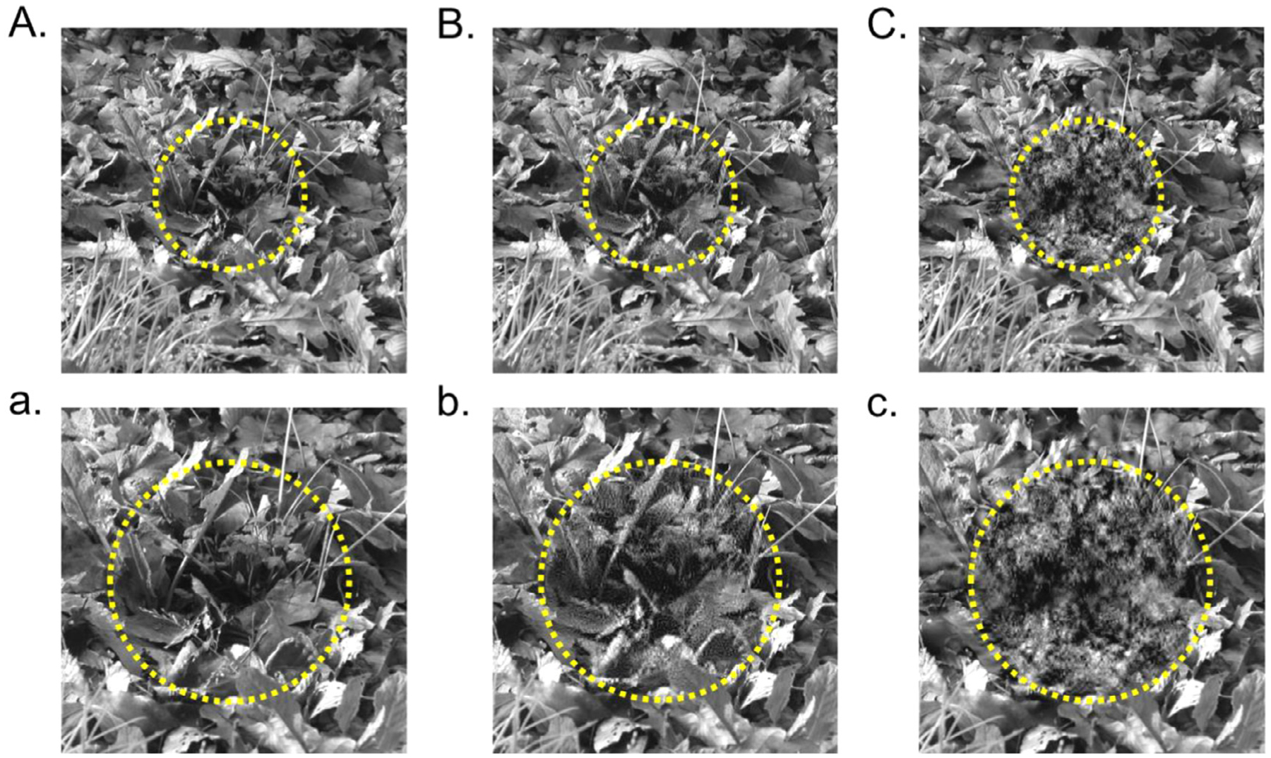
Using wavelets to degrade a spatially-restricted area. (A) Intact natural image with dashed circle denoting the targeted foveal region. (B) Natural image with only fine scale structure degraded near the fovea. (C) Natural image with all structure degraded near the fovea. Lowercase a-c show zoomed-in views of the central regions in A-C.

2.3. Extension to color images

The wavestrapping approach can be extended to color images (Fig. 4A). However, the addition of color information does require further considerations. While each pixel in a grayscale image can be described by a single number (intensity), color images contain three numbers per pixel - one for each color channel: red, green, and blue. The simplest extension of the above randomization techniques to a color image is to degrade the spatial structure in each channel independently. However, doing so does not preserve the color palette (Fig. 4B). To preserve the original colors (the color equivalent of preserving the pixel amplitude distribution), the image structure within each channel needs to be permuted in the same way across channels. In practice this can be achieved by permuting the detail coefficients within each color channel beginning with the same random seed (Fig. 4C).

Fig. 4.

Application to color images. (A) Intact natural image with RGB color channels. (B) Image with color channels degraded independently. (C) Image with color channels degraded identically. Note that the color palette is preserved in C but not B. This can most easily be seen by the examining the body of the wombat, which is tannish/brown in both A and C but mottled with red, green, and blue patches in B. Lowercase a-c show a zoomed-in view of the images for closer examination. Source photo from author A.M.P.

2.4. Extension to naturalistic movies

The above principles can be extended to dynamic natural scenes - i.e., film stimuli. In this case there is the additional dimension of time. Film stimuli incorporate the rich temporal variations in our environment and hence can provide a more engaging and ecologically-valid naturalistic experience than traditional static images (Hasson et al., 2004; Roberts et al., 2013; Sonkusare et al., 2019). The key consideration then is how to handle the temporal domain alongside the degradation of the spatial dimensions. One simple possibility is to permute the (spatial) wavelet coefficients within each frame independently, breaking the temporal structure associated with the scrambled spatial scales. However, this whitens the temporal spectra - introducing spurious high frequencies - as each frame differs abruptly from the preceding one. To fully preserve the temporal structure, one can use the same random seed for each frame (and for color videos, within each color channel too). Even with all spatial scales scrambled, preserving the temporal structure leaves an “imprint” of moving objects within the scene, as well as pans and cuts (see Supplementary Material S2, Sup Movie 1 for an example). Given the importance of motion to the visual system - including the “biological motion” of humans (Allison et al., 2000; Schultz and Pilz, 2009) - this preservation of apparent motion is crucial when permuting dynamic films in the wavelet domain to study the visual cortex.

This second strategy of a constant random seed destroys higher order statistics in the spatial domain but leaves those in the temporal domain exactly preserved. Wavelet resampling can also be applied in the temporal domain, treating the video as a single multidimensional time series, rather than as a series of discrete two-dimensional images. Notably, temporal variance of dynamic natural scenes also possesses a 1/f^α amplitude spectrum (Fig. 5A). This spatio-temporal wavestrapping can be achieved in two steps: parallel two-dimensional spatial resampling followed by parallel one-dimensional temporal resampling (Fig. 5B). Alternatively, the entire film could be wavestrapped using a single three-dimensional DWT following the same principles as wavestrapping a single three-dimensional spatial object (such as a single whole-brain fMRI volume (Breakspear et al., 2004)), although this mixes together information from the spatial and temporal domains.

Fig. 5.

Extension of wavestrapping to movies. (A) Temporal spectrum from a film clip shown as the power spectral density (PSD) across temporal frequency. Note that the spectrum was calculated from the red channel, middle pixel of Supplementary Movie 1 using a 10 second window and 50% overlap. (B) Schema for two-step wavestrapping of films. In Step 1, each frame and at each time point is spatially resampled (indicated by orange arrows). The resampling procedure is identical at the same scale for each time point and each frame. In Step 2, the time series from each pixel from the spatially wavestrapped data is resampled in the temporal dimension (indicated by yellow arrows). The resampling procedure at the same scale for each voxel is identical. All resampling is performed in the wavelet domain after appropriate wavelet decomposition (two-dimensional for Step 1 and one-dimensional for Step 2).

Using wavelets to manipulate movie data in the time domain can also adopt extensions outlined above for spatial images - namely focusing on high or low temporal scales and/or choosing specific temporal moments (such as scene transitions) and leaving other blocks unchanged. Temporal resampling can also extend to the parallel stream of audio information.

2.5. Thermodynamics of natural scenes

Recent work has shown that static (Saremi and Sejnowski, 2013) and dynamic (Munn and Gong, 2018) natural scenes possess the statistical hallmarks of criticality - that is, they reside close to a phase transition (i.e., a statistical boundary) between order and disorder. Computational analyses of natural scenes using the methods of statistical mechanics has suggested that this phase transition resides within specific latent layers of a natural scene (Saremi and Sejnowski, 2013) and is associated with thermodynamic “frustration” (see Supplementary Material, S3). By residing near these phase transitions, natural scenes are able to reflect a critical balance between (1) the ordered arrangement of the contours, edges, and textures of various sizes that endow it with structure and information and (2) the idiosyncratic and haphazard nature of this arrangement into the objects that characterize any specific scene and hence yield its semantic meaning and unique visual impression.

By applying our wavestrapping approach progressively it is possible to demonstrate the balance between order and disorder inherent to natural images (Fig. 6). This is because the randomization can be realized in varying degrees of depth, from just a few permuted coefficients up to full permutation. This is achieved by selecting random subsets of coefficients for permutation, leaving others invariant. Fig. 7A and Movie 1 both demonstrate the process of progressively disordering a natural image, which can be thought of as “heating” the scene. As can be seen in Fig. 7B, the amount of variability between realizations increases monotonically with the depth of randomization. Note that fully randomized realizations (i.e., randomization depth of 100%) are the most highly variable - akin to a gas. These highly variable realizations can be appreciated if one “boils” the scene (i.e., continues to randomize at a depth of 100% - see Movie 2). However, incremental permutations do show scale-specific expressions of variability (Fig. 7C) which differ between scenes. That is, despite their featureless 1/f spatial spectra, each natural scene has a distinct signature of increasing variability at different scales. Incremental wavelet resampling thus unpacks the latent statistical frustration within natural scenes which is not uniform across scales and scenes.

Fig. 6.

(A) Images used to demonstrate the thermodynamic properties of natural scenes. (B) Variability vs. wavelet scales. Each colored line is a single permutation of the corresponding image at one scale. Image variability is measured as the root mean squared differences between the original and scrambled image across pixels. Black lines show image averages. (C) Mean (black) across all four images ± standard deviation (red). There are no trends in mean image variability.

Fig. 7.

(A) Wavelet-based randomization (“heating”) of a natural scene, increasing incrementally from the original scene to fully randomized in steps of 25%. (B) Variability amongst an ensemble of random realizations increases monotonically with increasing depth of randomization at all scales. (C) However, some scales (here fine and coarse) show slightly greater variability with randomization than others (here mid-scales).

The wavelet-based randomization (or heating) can easily be reversed. For example, Movie 3 shows the process of “cooling” the scene back down from a boil (i.e., a fully randomized state) to its natural state. Interestingly, we can then continue to cool the image beyond its natural state and hence approach a single ordered state - akin to a solid (Movie 4). This process of “freezing” is further demonstrated in Fig. 8A, which shows the process of progressive ordering of a natural image. As can be seen in Fig. 8B, the amount of variability between realizations increases to a maximum at approximately 50% of wavelets ordered, corresponding to a mixture of natural and ordered phases, then decreases again as the single ordered state is approached. Similar to the process of randomization, the incremental ordering permutations do show scale-specific expressions of variability (Fig. 8C) which differ between scenes. Finally, we can “thaw” a frozen image (i.e., in a 100% ordered state) to its original, natural state (Movie 5) by progressive randomization (or heating) as described above.

Fig. 8.

(A) Wavelet-based ordering (“cooling”) of a natural scene, increasing incrementally from the original scene to fully ordered in steps of 25%. (B) Variability amongst an ensemble of realizations increases to a maximum at approximately 50% of wavelets ordered, corresponding to a mixture of natural and ordered phases, then decreases again as the single ordered state is approached. (C) Some scales show greater variability with ordering than others.

Fig. 9 further demonstrates the notion of natural image thermodynamics with natural images being positioned at a critical phase between fully ordered and disordered states. Subtle manipulations of dynamic natural scenes, using wavelet resampling to parametrically disrupt the complex statistics of their criticality whilst measuring cortical dynamics, represents an elusive but untested means of understanding how the structure of cortical dynamics are tuned adaptively to those of the natural world. Interestingly, the “critical” nature of dynamic natural scenes (i.e., that they are perched between order and disorder reflecting the balance of scene stability and sudden, spontaneous transitions) mirrors the critical, avalanche-like dynamics that occur throughout cortical systems (Cocchi et al., 2017). Incremental disruption - both “heating” (randomizing) and “cooling” (ordering) - allows tuning of a natural scene through its critical point and could be used in conjunction with imaging or neurophysiological recordings to further explore this intriguing area.

Fig. 9.

Natural images (middle column) reside near a critical boundary between order and disorder. Incremental, wavelet-based randomization (or heating) and ordering (or cooling) lead to fully disordered (right most column) vs. fully ordered states (left most column), respectively. Sandwiched between the images are plots of the variability seen across both scale and the depth of ordering or randomization when cooling or heating the natural image.

3. Probing the visual hierarchy - an fMRI demonstration

We conducted an fMRI experiment to illustrate the application of wavelet-based manipulations of natural images to probe the functional architecture of the visual hierarchy. As outlined above, there are numerous potential ways to manipulate static and dynamic natural scenes using wavelets. We designed a parametric, passive-fixation task to demonstrate some of the practical considerations of performing an fMRI experiment using wavelet-degraded stimuli (e.g., number of conditions can multiply quickly, use of a fixation task aimed at controlling attentional resources, etc.). Our proof-of-principle application to a visual fMRI experiment builds upon prior research in this field with the overarching goal being to contrast levels of cortical activity in different visual regions elicited by the presentation of intact natural images vs. wavelet-degraded natural images. Importantly, the basic image properties (luminance, spectra) remain the same between the two image types; only the higher-order statistical dependences (i.e., the structure of that image content) differ. To control for possible transition effects between (natural and wavestrapped) stimuli, we designed a factorial experiment which counterbalances the nature and order of their presentation.

Although primarily demonstrative, the experiment was motivated by a central hypothesis: that higher visual areas would be more sensitive to the complex structure present in natural images than lower visual areas. This was motivated by decades of previous research showing that primate visual cortex is organized hierarchically, with neurons responding to increasingly complex features as one progresses up the cortical hierarchy (DeYoe and Van Essen, 1988; Felleman and Van Essen, 1991; Van Essen, 2004).

3.1. Materials and methods

3.1.1. Subjects

Seven, right-handed participants (22–24 years, mean 22.9 years; 3 male, 4 female) who disavowed a history of neurological or psychiatric diseases completed a functional neuroimaging experiment. All participants had normal or corrected to normal vision. The experiment was conducted with the written consent of each participant following approval by the local human research ethics committee in accordance with national guidelines.

3.1.2. Experimental design

Stimuli were presented in blocks of 8 s while participants fixated on a small superimposed crosshair. Stimuli consisted of natural images, degraded images obtained through wavestrapping these natural images at select (fine or coarse) scales, and colored noise control images matched for luminance and spectra content obtained through wavestrapping the natural images at all spatial scales.

A partial 3 × 2 × 2 within-subjects factorial design was used. The independent variables were type of image manipulation (N1: degrade from natural image, N2: degrade from noise, N3: restore from noise), spatial scale manipulated (S1: fine and S2: coarse), and presentation of manipulation (F1: flip vs. F2: flick). All experimental conditions are summarized in the Supplementary Material (S2, Table 1), with representative conditions described in detail below:

• N1,S1,F1 - the fine scale information (S1) of a natural image was permuted (N1). This resulted in the degradation of the structure at that scale and hence a natural image with all scales of structure intact except the fine scale. The experimental block involved flipping back and forth (F1) between the original image and the degraded image.

• N1,S2,F2 - the coarse scale information (S2) of a natural image was permuted (N1). This resulted in the degradation of the structure at that scale and hence a natural image with all scales of structure intact except the coarse scale. The experimental block involved flicking through (F2) a series permutations of the same source image (i.e., the permutation was carried out a number of times on the same natural image, and were presented in succession during the imaging block).

• N2,S2,F2 - the coarse scale information (S2) of a noise image was permuted (N2). Since we began with a noise image, there was no natural scene structure to degrade; however, the permutation was identical to what was performed on a natural image and leads to a slightly distinct noise image that differs only at the targeted spatial scale. The experimental block involved flicking through (F2) a series of permutations on the same source image.

• N3,S2,F1 - the coarse scale information (S2) from a natural image was put into a noise image (N3). The experimental block involved flipping back and forth (F1) between the original noise image and the noise image with structure added.

These stimuli permutations were designed to parametrically control the depth of image manipulation and the spatial scale targeted while controlling for the effects of image transitions. The factorial design was incomplete (partial) in that it was not possible to test the flick presentation type (F2) for the condition that involved adding structure to a noise image (N3). That is, for any given natural scene there is only one possible instance of structure that can be added to remain faithful to the original scene (i.e., any alteration of this structure would change the scene). In contrast, there is no limit to the number of instances of noise images that can be constructed from each natural scene due to the randomized nature of the wavestrapped permutations. In addition to the above conditions (all of which involve a changing stimulus, whether flipping or flicking), we also included two static image block types: a natural image (N1, S0, F0) and a noise image (N2, S0, F0). An isoluminant gray background was shown as a baseline block.

In total then, there were 12 different experimental block types and a baseline. Each block was presented three times per scan run. All experimental blocks were presented for 8 s and the gray background baseline was presented for 12 s. During the ON period for the stimulus blocks with image change (i.e., flip or flick), the transition occurred every 0.5 s. The block types were pseudo-randomized except that we ensured that each block type followed the gray background baseline condition an equal number of times and that the last block of every run was the gray background condition to permit the fMRI signal to return to baseline. 12 runs were collected per subject, in a single scan session.

To control attention, aid fixation, and monitor subject alertness, a color/orientation conjunction task was performed at fixation throughout the entire run (Puckett and DeYoe, 2015; Treisman and Gelade, 1980). For this purpose, a small circle (10 × 10 pixels, subtending 0.15° visual angle) was superimposed upon the images. The circle contained a pattern that randomly changed every 2 s among 4 possible configurations: red horizontal, red vertical, green horizontal, and green vertical. The participant was required to report the nature of each change via one of two button presses (button 1 = red horizontal or green vertical, button 2 = red vertical or green horizontal). In addition to the color/orientation patch, a fine grid was overlaid on the images to aid fixation (Schira et al., 2007).

An example of the visual stimulus and block paradigm (with annotation), is presented in the Supplementary Material (S2, Sup Movie 2).

3.1.3. image manipulation

Stimuli were constructed by manipulating a set of natural images using the wavelet transform (as outlined in Section 2). The natural images were sourced from the “Zurich natural images” database, which is freely available for academic use (Einhauser and Konig, 2003). Note that the subset of images from this database used here are shown in the Supplementary Material (S2, Sup Figs. 1 and 2). In general, constructing the stimuli involved: converting the RGB image to greyscale, permuting the detail coefficients at a specific spatial scale (or scales) using the wavelet transform, resizing the image (to 768 × 768, subtending 11° visual angle), and then adjusting the luminance values so that the resampled amplitude spectra matched those from the original natural images. More specifically:

• To degrade a single spatial scale of natural image structure (factor N1), we permuted the coefficients associated with one of two spatial scales (i.e., levels): fine (S1) and coarse (S2). Note that the coefficient levels corresponding to fine and coarse natural image structure are dependent on the input image size and were determined empirically. For this, we permuted the coefficients across a series of levels and chose the two levels corresponding to fine and coarse natural image structure by visual inspection. Note that the fine scale manipulation targeted structure in the range of 4.5 – 8.8 cycles per degree and the coarse scale manipulation targeted structure in the range of 1.3 – 2.4 cycles per degree.

• To construct noise images that shared the same basic image properties as our natural images (factor N2), we simply performed the wavelet degradation on the natural images across all spatial scales. This destroys all natural image structure, leaving a noise image with the same 1/f^α frequency distribution as the original natural image.

• To put natural image back into a noise image (factor N3), we first degraded all the spatial scales except that of interest (i.e., all but S1 or S2). Then we degraded the remaining structure at that scale. This produced a pair of images: one noise image (all scales permuted) and another that was identical to the noise image except that one spatial scale of information still remained.

All wavelet resampling was performed using Daubechies wavelets, which are a family of orthogonal wavelets characterized by a maximal number of vanishing moments while minimizing asymmetry (here we used the db6 wavelet with 6 vanishing moments). To avoid edge effects when performing the wavelet degrading, which manifest as sharp horizontal or vertical striping in the image, we did not perform the wavelet degradation over the entire image. Instead, we left an outer border (1/20th of the image size) untouched around the entire image. After the detail coefficients associated with spatial locations inside this border were permuted, the image was cropped so that only the permuted portion remained.

3.1.4. Retinotopic localizer

To localize cortical responses to visual images, we performed two types of phase-encoded retinotopic mapping: one to map polar angle and the other to map eccentricity representations. Briefly, the polar angle stimulus consisted of a rotating bowtie (two wedges opposite one another and meeting at fixation) and the eccentricity stimulus consisted of an expanding ring (Schira et al., 2009). The aperture contained one of three colored texture patterns (checkers, expanding and contracting spirals, or rotating sinusoidal gratings) which changed randomly every 250 ms. Participants performed a fixation color detection task at a central maker, and a fixation grid was overlaid atop the stimuli.

3.1.5. Magnetic resonance imaging data acquisition

Data were acquired on a Philips 3T Achieva X Series equipped with Quasar Dual gradients and a 32-channel head coil. Whole-brain, anatomical images were collected using a magnetization-prepared rapid acquisition with gradient echo MPRAGE sequence with a TE of 2.8 ms, TR of 6.3 ms, flip angle of 8°, FOV of 256 mm × 256 mm, a matrix size of 340 × 340, and 250 slices that were 0.75 mm thick - resulting in an isotropic voxel size of 0.75 mm.

The voxel resolution of the functional echo planar images (EPIs) collected here was 1.5 × 1.5 × 1.5 mm³ across 31–32 oblique coronal slices covering the occipital pole. EPIs were acquired with a TR of 2 s, a TE of 25 ms, a SENSE factor of 2, a 128 × 128 matrix (ascending acquisition), and a FOV of 192 mm. For polar angle mapping 186 vol were collected, for eccentricity mapping 174 vol were collected, and for the natural image experiment 184 vol were collected. Before data analysis, the first few volumes were discarded to account for the high T1 saturation that occurs at the beginning of a scan. For both mapping protocols the first 6 vol were discarded, and for the natural image experiment the first 4 vol were discarded.

3.1.6. Data analysis

Pre-processing of the functional data was performed using SPM8 (SPM software package, Wellcome Department, London, UK; http://www.fil.ion.ucl.ac.uk/spm/). Data were motion corrected using a rigid body transform and 7th degree B-spline interpolation. Images were slice scan time corrected using the first image as the reference slice and resliced into the space of the first image.

For retinotopic mapping, “traveling-wave” analysis procedures were conducted using the mrVista Toolbox (Stanford University, Stanford, CA; http://white.stanford.edu/software/). The cyclic retinotopic mapping data was analysed using a fast Fourier transform based correlation analysis, as built in the mrLoadRet software from the mrVISTA toolbox. This estimates a coherency value for each voxel in the cortex as a ratio between the power at the stimulus frequency and noise. The retinotopic location (both polar angle and eccentricity) for each voxel was determined by the phase value at the stimulus frequency. The retinotopy data were then displayed on a 3D rendered brain surface (Engel et al., 1997; Schira et al., 2009).

Volumetric segmentation of white matter was performed manually using ITK Gray (Yushkevich et al., 2006). 3D surface reconstructions of the left and right hemisphere were generated using mrMesh (a function within the mrVista Toolbox) by growing a 3-voxel thick layer (1.5 mm isotropic voxels) above the gray/white boundary. To improve data visualization (i.e. when projecting functional data onto surfaces), these surfaces were also computationally-inflated using the “smoothMesh” option in mrMesh (8 iterations). Note that the cortical surface models were only used for data visualization and region-of-interest (ROI) definition. All analyses and statistics were performed using the volumetric data.

Further analysis in the mrVista Toolbox included a general linear model (GLM) of responses across early visual areas (V1, V2, V3) for each individual subject. The Boynton Gamma HRF was used to model the haemodynamic response function (Boynton et al., 1996). All runs were concatenated and the null gray background condition was used as baseline.

3.2. Results

We first used the retinotopic mapping data to define V1, V2, and V3 ROIs in both hemispheres for each individual (Fig. 10). We then extracted the GLM-derived β-weights associated with each experimental condition from all voxels in each ROI. The mean β-weight was then computed for each visual area, combining both hemispheres.

Fig. 10.

Defining visual area ROIs. For each individual subject, early visual cortex was partitioned into V1, V2, and V3 ROIs using polar angle retinotopic mapping data. On the far left is an inflated cortical surface model for the left hemisphere of a single subject. Next to that is a zoomed-in view of the occipital cortex showing the polar angle retinotopic map (un-thresholded). On the right is the same zoomed-in view of the occipital cortex, showing the three visual area ROIs overlaid upon the curvature pattern.

Fig. 11A shows the average response in each of the visual area ROIs for each condition across all subjects. Inspection of Fig. 11A reveals a few salient, interesting response differences across visual areas and across experimental conditions. Notably, as one progresses up the visual hierarchy (V1 → V2 → V3), the response amplitude decreases across all conditions. It also appears that, in general, the natural images elicit greater activation than the noise images (N1>N2,N3). This is true not only for the conditions involving image manipulation, but also for the no manipulation conditions (N1,S0,F0 vs. N2,S0,F0). However, the degree of difference between natural image (N1) vs. noise image (N2) conditions appears to become greater as one progresses up the hierarchy.

Fig. 11.

Activation across the early visual hierarchy for intact vs. degraded natural images. (A) Group averaged β-weights for all experimental conditions in each visual areas ROI. Error bars represent SEM across individuals. (B) β-weights in each visual area ROI for the different types of image manipulations (N1: degrade from natural image, N2: degrade from noise, N3: restore from noise), collapsed across all other factors. (C) β-weights across eccentricity for both scale conditions in each visual area, collapsed across other factors. Ecc 1 to Ecc 6 range from the fovea to the periphery (0.06 ≤ Ecc 1 ≤ 0.48; 0.48 ≤ Ecc 2 ≤ 0.95; 0.95 ≤ Ecc 3 ≤ 1.36; 1.36 ≤ Ecc 4 ≤ 1.93; 1.93 ≤ Ecc 5 ≤ 2.74; 2.74 ≤ Ecc 6 ≤ 3.89°). For (B) and (C), whiskers with caps show min/max, bottom and top edges of boxes indicate 25th and 75th percentile, and central line marks the median across all participants.

Qualitative assessment of Fig. 11A appears to support the core hypothesis that higher cortical areas are more sensitive to more complex statistical features of natural scenes than V1 (i.e., cortical areas respond more strongly when natural image structure is present than when absent and this difference increases as one progresses up the hierarchy). To test this, we collapsed the data across the spatial scale (S1 and S2) and presentation (F1 and F2) factors, and removed the static, no manipulation conditions (N1,S0,F0 and N2,S0,F0; Fig. 11B). We then performed a 2-way repeated measures ANOVA to investigate if the visual areas differentially responded to the different image manipulations (N1, N2, and N3). We found that a differential response was indeed present. That is, in addition to significant main effects for both visual area [F = 52.3, p<0.001] and the type of image manipulation [F = 11.2, p = 0.0018], there was also a significant interaction effect [F = 16.6, p<0.001]. Looking at Fig. 11B, it appears that the interaction effect reflects an increasing effect of natural image structure on the responses as one progresses from V1 to V3. Recall that N1 is a natural image with one scale of structure degraded, N2 is essentially a noise image (all scales of structure degraded), and N3 is mostly a noise image but still has one scale of structure present. Hence, N1 has the most natural image structure, N3 the second most, and N2 has the least. In V1, there is little difference among the three conditions suggesting that V1 is only weakly influenced by the presence versus absence of the higher-order correlations that characterize natural image structure. In V2, however, the effect of image type on the average response becomes stronger and appears graded by the amount of structure present. This same differential response is further pronounced in V3.

Sensitivity to different spatial scales is known to vary as functions of both visual area and eccentricity. That is, receptive field size increases up the visual hierarchy and at increasingly peripheral eccentricities (Dumoulin and Wandell, 2008). We hence also explored the effect of the scale condition (S) and its interaction with visual area and eccentricity. For this, we first sub-divided each visual area ROI into 6 eccentricity bands using the retinotopic mapping data (0.06 ≤ Ecc 1 ≤ 0.48; 0.48 ≤ Ecc 2 ≤ 0.95; 0.95 ≤ Ecc 3 ≤ 1.36; 1.36 ≤ Ecc 4 ≤ 1.93; 1.93 ≤ Ecc 5 ≤ 2.74; 2.74 ≤ Ecc 6 ≤ 3.89°). We collapsed the data across the presentation (F1 and F2) and image manipulation (N1, N2, and N3) factors, and removed the static, no manipulation conditions (Fig. 11C). We then performed a 3-way repeated measures ANOVA finding a significant main effect again for visual area [F = 37.0, p < 0.001] as well as significant main effects for eccentricity [F = 3.5, p = 0.014] and scale [F = 80.6, p < 0.001]. There were also significant interaction effects between visual area and eccentricity [F = 3.3, p = 0.002] as well as between eccentricity and scale [F = 4.5, p = 0.004] but not between visual area and scale [F = 1.3, p = 0.303] nor among the three [F = 0.6, p = 0.804]. Looking at Fig. 11C, the main effects are clear. For visual area, we see a general diminishing of the response as one progresses up the visual hierarchy (similar to the effect of area seen in Fig. 11B). For eccentricity, we see a the same basic inverted-U pattern across eccentricity for each combination of spatial scale condition and visual area except for the fine scale condition in V3 (likely driving the interaction effect). For the scale condition, we see consistently greater responses to the coarse scale manipulation compared to the fine scale (also clearly seen in Fig. 11A), particularly at intermediate eccentricities.

With respect to the scale effect, note that the process of wavestrapping a noise image (N2) simply results in another noise image since no structure was originally present. However, it is important to understand that the resulting noise image is still different from the source noise image, and the difference is dependent on the manipulated scale. Therefore, when the images are presented by flicking between or flipping through the different instances, changes in the image occur at the targeted spatial scale. From our results then, it appears that when the changes occur at the coarse scale, a higher degree of activity is seen in visual cortex compared to when the changes occur at the fine scale. The perceptual difference between the fine and coarse scale resampling of noise can be seen by contrasting conditions N2,S1,F1 vs. N2,S2,F1 or N2,S1,F2 vs. N2,S2,F2 in Supplementary Movie 2.

Note that the primary motivation for ‘flipping’ or ‘flicking’ across multiple instances within a block was to make the stimuli “dynamic” and hence more salient to the visual system compared to using a static image across the block duration. The choice of flipping versus flicking was selected to probe the role of prior context on visual responses -i.e. whether a statistical violation (the wavelet-degraded scale) would have a greater cortical salience when introduced in and out of a preserved scene (F1), or whether the violation would accrue a stronger response when continually presented (F2). Whereas the dynamic conditions did elicit greater responses than their corresponding static conditions (Fig. 11A), we did not find any main effect of the presentation factor (F1 vs. F2) [F = 0.2, p = 0.681] nor an interaction with visual area [F = 3.4, p = 0.067] when conducting a 2-way repeated measures ANOVA.

4. Discussion

Sensory and cognitive neuroscience has traditionally employed simple, abstract, and narrowband stimuli to examine cortical response properties. These stimuli have served the field well, offering a way to tightly control variables of interest and leading to an extensive characterization of the response of single neurons and populations of neurons to basic image properties such as luminance, contrast, orientation, and spatial frequency. Despite this, these stimuli lack ecological validity as they rarely come close to approximating the types of stimuli encountered in typical sensory experiences outside of experimental conditions. Pertinently, there is mounting evidence suggesting that the cortex may be more strongly ‘tuned’ to the statistical properties of naturalistic stimuli (for review, see Sonkusare et al., 2019). For example, a recent study (Isherwood et al., 2017) using broadband noise stimuli observed that stimuli with 1/f^α spectra close to that of natural scenes (i.e., α = 1.25, Fig. 1C) elicited stronger BOLD responses than stimuli with 1/f^α spectra outside of the natural range (i.e., α = 0.25 or α = 2.25). Interestingly, this apparent tuning of the cortex to the spectra of natural stimuli is mirrored by visual sensitivity and preference at the behavioral level. Discrimination sensitivity, detection sensitivity, as well as aesthetic preference are highest for noise stimuli with natural 1/f^α spectra and lowest for unnatural 1/f^α spectra (Spehar and Taylor, 2013; Spehar et al., 2015). This supports the notion that the visual system is tuned to the statistical properties of natural scenes. Findings such as these highlight the importance of using more complex, naturalistic stimuli in neuroscientific pursuits.

The benefit of complementing studies using traditional, abstract stimuli with those that use more ecological stimuli is clear. The use of naturalistic stimuli, however, is still relatively nascent, and as such, considerable challenges remain. One such issue is determining how to manipulate these naturalistic stimuli with sufficient control and rigor. Seminal early work disrupted the temporal narrative by sharp block shuffling of movie segments in the time domain to unveil large-scale temporal hierarchies in the cortex (Hasson et al., 2008). The wavelet approach outlined in the present manuscript offers an alternative, more nuanced opportunity in this direction to turn the focus on hierarchies in the visual system. Our work demonstrates that it is possible to parametrically and subtly manipulate the complex statistical properties of natural scenes with a high degree of control and flexibility - and that the visual system is sensitive to these subtle manipulations.

There are a wide range of ways that wavelets can be used to manipulate stimuli to probe functional effects of natural scene statistics in the visual hierarchy, some of which were described in Part 1. The neuroimaging study here (Part 2) makes use of one of these, demonstrating some of the practical considerations of performing an fMRI experiment using wavelet-degraded stimuli. In doing so, we found evidence in support of our main hypothesis (that higher hierarchical regions in visual cortex are more sensitive to natural scene statistics). These results are convergent with other recent research, using substantially different visual stimuli, showing that sensitivity to the distinctive higher-order correlations of natural scenes begins to arise in visual area V2. For example, Freeman et al. (2013) found that generated, naturalistic texture stimuli (with higher-order correlations) differentially modulated cortical responses in V2 but not V1 compared to spectrally matched noise (without the higher-order correlations). Notably, comparable results were found by the authors using both fMRI in humans and neural recordings in macaque. Yu et al. (2015) similarly showed that many neurons in macaque V2 (but few in V1) are sensitive to higher-order properties of natural scenes. Rather than degrading natural images as done in the present study or constructing stimuli that mimic naturalistic textures (Freeman et al., 2013), Yu et al. used binary textures that were highly unnatural, but isolated specific multipoint correlations characteristic of natural images (i.e., the statistics of the combinations of luminance values that appear in several points of a natural image) (Hermundstad et al., 2014; rkacik et al., 2010). Note that the uniform textures generated by Freeman et al. (2013) appears more “natural” than the binary textures (Yu et al., 2015), although both can be easily visually disambiguated from an actual natural image as they lack the contextual information and complex variability present in natural scenes. It is clear then, that although selectivity to higher-order correlations in natural images begin to arise in V2, future work is required to determine where along the hierarchy further selectivity to additional natural image structure emerges.

The human visual system is composed of many functionally distinct cortical visual areas (Grill-Spector and Malach, 2004; Zeki et al., 1991). Sensory-driven responses tend to decrease as one progress up the visual hierarchy, and as such, our finding that responses to all of our stimuli decrease as one progresses up the visual hierarchy is unsurprising. Notably, however, we also found that the higher cortical areas appear to be more sensitive to the complex visual features - that is, the decrease in responses up the visual stream was more pronounced for wavelet resampled stimuli. The present application to fMRI data thus suggests that the higher order structure being degraded by the wavelet technique is directly related to the complex features that the higher visual areas encode. That is, cells along the visual hierarchy become increasingly sensitive to the conditional dependences among multiple neurons in lower hierarchical levels, mirroring the complex conditional dependences in unaltered natural scenes. Presumably, this effect would be stronger in even higher-order areas; however, our data are insufficient to test this. Due to the size and orientation of our fMRI acquisition slab, we only have partial coverage of hV4 for most participants. In addition, time constraints restricted the number of runs of each retinotopic mapping stimulus - limiting the data quality and thus our ability to confidently demarcate higher-order dorsal and lateral areas. Future studies could be designed to circumvent this issue, for example by having a separate scan session dedicated to the collection of a comprehensive, high-quality retinotopic mapping dataset.

One powerful aspect of the wavelet-based approach outlined here is the ability to target structure at specific spatial scales. As mentioned, receptive field size and hence spatial frequency sensitivity is known to vary both across visual areas as well as across eccentricities within a visual area (Dumoulin and Wandell, 2008; Yoshor et al., 2007). By combining the experiment with fMRI-based estimates of population receptive field sizes (Dumoulin and Wandell, 2008; Zeidman et al., 2018), future studies will be able to take a more detailed look at the relationship between cortical activity related to specific scales of natural image structure and the underlying receptive field sizes. Our preliminary results suggest that manipulations to coarse scales elicit stronger results across the visual cortex than manipulations to the small scales. Interestingly, this is found when wavestrapping the noise images (N2) as well as those with structure present (N1). Although the mean perturbation across the images and realizations do not show a scale-specific effect, the variability is higher at coarser scales (see Fig. 11). Hence the greater responses to coarse scale manipulations (S2) compared to the fine scale manipulations (S1) may either reflect stronger neuronal sensitivity to coarse scale information or encoding of the trial-to-trial variability. In studying the effect of scale, it will also be important to test across the full range of spatial scales, rather than only two as done in the present study. Full-range, parametric studies are necessary to reveal any important non-monotonicity that might be present in the response properties (Rainer et al., 2001).

Although participants in our experiment attended to a fixation task while passively viewing raw and altered static natural images presented in successive transitions, it is important to note that perception in the wild is embedded in a broader action-perception cycle (Fuster, 2002). It thus makes sense to not only use wavelet resampling to degrade the spatial and temporal statistics, but to do so while participants freely view movies (i.e., with unrestricted eye movements). As reviewed above, wavelet resampling is directly applicable to dynamic, spatio-temporal stimuli (S2, Sup Movie 1) - and there exists several different ways of achieving this: preserving, destroying, or manipulating the complex temporal statistics embedded in dynamic natural scenes. Block resampling is one variant of this broader class, preserving the temporal structure within blocks but degrading the temporal spectra - precisely and only at the time-scale of the block.

As a final consideration, image manipulations of higher order statistics could be made at the time of saccades, during fixational eye movements, or during scene transitions - introducing subtle stimulus errors into the active stream of visual perception, while avoiding low-level changes in luminance, contrast, or spectra. This inclusion of parametric prediction errors would allow novel probes of the predictive coding principles of visual function (Edwards et al., 2017; Friston, 2005; Vetter et al., 2012). Other recent work has used wavelet resampling to construct dynamic stimuli from a static natural scene by cyclically permuting the wavelet scales, hence tuning a static scene in and out of its (preserved) noise context (Koenig-Robert and VanRullen, 2013; Koenig-Robert et al., 2015). This approach allows cyclic presentation of both expected and surprising semantic content (of the natural scene) while keeping the spectral properties of the stimulus constant (unlike a traditional event related paradigm), thus probing cortical hierarchies for their role in predictive coding and error responses (Gordon et al., 2019a, 2017, 2019b).

References

- Allison T, Puce A, McCarthy G, 2000. Social perception from visual cues: role of the STS region. Trends Cogn Sci 4, 267–278. [DOI] [PubMed] [Google Scholar]
- Boynton GM, Engel SA, Glover GH, Heeger DJ, 1996. Linear systems analysis of functional magnetic resonance imaging in human V1. J Neurosci 16, 4207–4221. [DOI] [PMC free article] [PubMed] [Google Scholar]
- Breakspear M, Brammer MJ, Bullmore ET, Das P, Williams LM, 2004. Spatiotemporal wavelet resampling for functional neuroimaging data. Hum Brain Mapp 23, 1–25. [DOI] [PMC free article] [PubMed] [Google Scholar]
- Bullmore E, Long C, Suckling J, Fadili J, Calvert G, Zelaya F, Carpenter TA, Brammer M, 2001. Colored noise and computational inference in neurophysiological (fMRI) time series analysis: resampling methods in time and wavelet domains. Hum Brain Mapp 12, 61–78. [DOI] [PMC free article] [PubMed] [Google Scholar]
- Burton GJ, Moorhead IR, 1987. Color and spatial structure in natural scenes. Appl Opt 26, 157–170. [DOI] [PubMed] [Google Scholar]
- Cocchi L, Gollo LL, Zalesky A, Breakspear M, 2017. Criticality in the brain: a synthesis of neurobiology, models and cognition. Prog Neurobiol 158, 132–152. [DOI] [PubMed] [Google Scholar]
- Dumoulin SO, Wandell BA, 2008. Population receptive field estimates in human visual cortex. Neuroimage 39, 647–660. [DOI] [PMC free article] [PubMed] [Google Scholar]
- Edwards G, Vetter P, McGruer F, Petro LS, Muckli L, 2017. Predictive feedback to V1 dynamically updates with sensory input. Sci Rep 7, 16538. [DOI] [PMC free article] [PubMed] [Google Scholar]
- Einhauser W, Konig P, 2003. Does luminance-contrast contribute to a saliency map for overt visual attention? Eur J Neurosci 17, 1089–1097. [DOI] [PubMed] [Google Scholar]
- Engel SA, Glover GH, Wandell BA, 1997. Retinotopic organization in human visual cortex and the spatial precision of functional MRI. Cereb Cortex 7, 181–192. [DOI] [PubMed] [Google Scholar]
- Field DJ, 1987. Relations between the statistics of natural images and the response properties of cortical cells. J Opt Soc Am A 4, 2379–2394. [DOI] [PubMed] [Google Scholar]
- Field DJ, 1994. What is the goal of sensory coding? Neural Comput 6, 559–601. [Google Scholar]
- Field DJ, 1999. Wavelets, vision and the statistics of natural scenes. Roy Soc of London Phil Tr A 357, 2527. [Google Scholar]
- Frazor RA, Geisler WS, 2006. Local luminance and contrast in natural images. Vision Res 46, 1585–1598. [DOI] [PubMed] [Google Scholar]
- Freeman J, Ziemba CM, Heeger DJ, Simoncelli EP, Movshon JA, 2013. A functional and perceptual signature of the second visual area in primates. Nat Neurosci 16, 974–981. [DOI] [PMC free article] [PubMed] [Google Scholar]
- Friston K, 2005. A theory of cortical responses. Philos Trans R Soc Lond B Biol Sci 360, 815–836. [DOI] [PMC free article] [PubMed] [Google Scholar]
- Fuster JM, 2002. Physiology of executive functions: the perception-action cycle. In: Stuss DT, Knight RT (Eds.), Principles of Frontal Lobe Function. Oxford University Press, New York, NY, US, pp. 96–108. [Google Scholar]
- Gordon N, Hohwy J, Davidson MJ, van Boxtel JJA, Tsuchiya N, 2019a. From intermodulation components to visual perception and cognition-a review. Neuroimage 199, 480–494. [DOI] [PubMed] [Google Scholar]
- Gordon N, Koenig-Robert R, Tsuchiya N, van Boxtel JJ, Hohwy J, 2017. Neural markers of predictive coding under perceptual uncertainty revealed with Hierarchical Frequency Tagging. Elife 6. [DOI] [PMC free article] [PubMed] [Google Scholar]
- Gordon N, Tsuchiya N, Koenig-Robert R, Hohwy J, 2019b. Expectation and attention increase the integration of top-down and bottom-up signals in perception through different pathways. PLoS Biol 17, e3000233. [DOI] [PMC free article] [PubMed] [Google Scholar]
- Graham D, Schwarz B, Chatterjee A, Leder H, 2016. Preference for luminance histogram regularities in natural scenes. Vision Res 120, 11–21. [DOI] [PubMed] [Google Scholar]
- Graps A, 1995. An introduction to wavelets. IEEE Comput Sci Eng 2, 50–61. [Google Scholar]
- Grill-Spector K, Malach R, 2004. The human visual cortex. Annu Rev Neurosci 27, 649–677. [DOI] [PubMed] [Google Scholar]
- Hasson U, Nir Y, Levy I, Fuhrmann G, Malach R, 2004. Intersubject synchronization of cortical activity during natural vision. Science 303, 1634–1640. [DOI] [PubMed] [Google Scholar]
- Hasson U, Yang E, Vallines I, Heeger DJ, Rubin N, 2008. A hierarchy of temporal receptive windows in human cortex. J Neurosci 28, 2539–2550. [DOI] [PMC free article] [PubMed] [Google Scholar]
- Hermundstad AM, Briguglio JJ, Conte MM, Victor JD, Balasubramanian V, Tkacik G, 2014. Variance predicts salience in central sensory processing. Elife 3. [DOI] [PMC free article] [PubMed] [Google Scholar]
- Hubel DH, Wiesel TN, 1959. Receptive fields of single neurones in the cat’s striate cortex. J Physiol 148, 574–591. [DOI] [PMC free article] [PubMed] [Google Scholar]
- Hubel DH, Wiesel TN, 1968. Receptive fields and functional architecture of monkey striate cortex. J Physiol 195, 215–243. [DOI] [PMC free article] [PubMed] [Google Scholar]
- Isherwood ZJ, Schira MM, Spehar B, 2017. The tuning of human visual cortex to variations in the 1/f(alpha) amplitude spectra and fractal properties of synthetic noise images. Neuroimage 146, 642–657, [DOI] [PubMed] [Google Scholar]
- Karklin Y, Lewicki MS, 2009. Emergence of complex cell properties by learning to generalize in natural scenes. Nature 457, 83–86. [DOI] [PubMed] [Google Scholar]
- Koenig-Robert R, VanRullen R, 2013. SWIFT: a novel method to track the neural correlates of recognition. Neuroimage 81, 273–282. [DOI] [PubMed] [Google Scholar]
- Koenig-Robert R, VanRullen R, Tsuchiya N, 2015. Semantic Wavelet-Induced Frequency-Tagging (SWIFT) Periodically Activates Category Selective Areas While Steadily Activating Early Visual Areas. PLoS ONE 10, e0144858. [DOI] [PMC free article] [PubMed] [Google Scholar]
- Munn B, Gong P, 2018. Critical Dynamics of Natural Time-Varying Images. Phys Rev Lett 121, 058101. [DOI] [PubMed] [Google Scholar]
- Olshausen BA, Field DJ, 1996. Emergence of simple-cell receptive field properties by learning a sparse code for natural images. Nature 381, 607–609. [DOI] [PubMed] [Google Scholar]
- Puckett AM, DeYoe EA, 2015. The attentional field revealed by single-voxel modeling of fMRI time courses. J Neurosci 35, 5030–5042. [DOI] [PMC free article] [PubMed] [Google Scholar]
- Rainer G, Augath M, Trinath T, Logothetis NK, 2001. Nonmonotonic noise tuning of BOLD fMRI signal to natural images in the visual cortex of the anesthetized monkey. Curr Biol 11, 846–854. [DOI] [PubMed] [Google Scholar]
- Roberts JA, Wallis G, Breakspear M, 2013. Fixational eye movements during viewing of dynamic natural scenes. Front Psychol 4, 797. [DOI] [PMC free article] [PubMed] [Google Scholar]
- Ruderman DL, Bialek W, 1994. Statistics of natural images: scaling in the woods. Phys Rev Lett 73, 814–817. [DOI] [PubMed] [Google Scholar]
- Saremi S, Sejnowski TJ, 2013. Hierarchical model of natural images and the origin of scale invariance. Proc Natl Acad Sci U S A 110, 3071–3076. [DOI] [PMC free article] [PubMed] [Google Scholar]
- Schira MM, Tyler CW, Breakspear M, Spehar B, 2009. The foveal confluence in human visual cortex. J Neurosci 29, 9050–9058. [DOI] [PMC free article] [PubMed] [Google Scholar]
- Schira MM, Wade AR, Tyler CW, 2007. Two-dimensional mapping of the central and parafoveal visual field to human visual cortex. J Neurophysiol 97, 4284–4295. [DOI] [PubMed] [Google Scholar]
- Schultz J, Pilz KS, 2009. Natural facial motion enhances cortical responses to faces. Exp Brain Res 194, 465–475. [DOI] [PMC free article] [PubMed] [Google Scholar]
- Sekuler AB, Bennett PJ, 2001. Visual neuroscience: resonating to natural images. Curr Biol 11, R733–R736. [DOI] [PubMed] [Google Scholar]
- Sonkusare S, Breakspear M, Guo C, 2019. Naturalistic stimuli in neuroscience: critically acclaimed. Trends Cogn Sci 23, 699–714. [DOI] [PubMed] [Google Scholar]
- Spehar B, Taylor RP, 2013. Fractals in art and nature: why do we like them?, Human Vision and Electronic Imaging XVIII. International Society for Optics and Photonics, 865118. [Google Scholar]
- Spehar B, Wong S, van de Klundert S, Lui J, Clifford CW, Taylor RP, 2015. Beauty and the beholder: the role of visual sensitivity in visual preference. Front Hum Neurosci 9, 514. [DOI] [PMC free article] [PubMed] [Google Scholar]
- Tkacik G, Prentice JS, Victor JD, Balasubramanian V, 2010. Local statistics in natural scenes predict the saliency of synthetic textures. Proc Natl Acad Sci U S A 107, 18149–18154. [DOI] [PMC free article] [PubMed] [Google Scholar]
- Tolhurst DJ, Tadmor Y, Chao T, 1992. Amplitude spectra of natural images. Ophthalmic Physiol Opt 12, 229–232. [DOI] [PubMed] [Google Scholar]
- Treisman AM, Gelade G, 1980. A feature-integration theory of attention. Cogn Psychol 12, 97–136. [DOI] [PubMed] [Google Scholar]
- van der Schaaf A, van Hateren JH, 1996. Modelling the power spectra of natural images: statistics and information. Vision Res 36, 2759–2770. [DOI] [PubMed] [Google Scholar]
- Vetter P, Edwards G, Muckli L, 2012. Transfer of predictive signals across saccades. Front Psychol 3, 176. [DOI] [PMC free article] [PubMed] [Google Scholar]
- Yoshor D, Bosking WH, Ghose GM, Maunsell JH, 2007. Receptive fields in human visual cortex mapped with surface electrodes. Cereb Cortex 17, 2293–2302. [DOI] [PubMed] [Google Scholar]
- Yu Y, Schmid AM, Victor JD, 2015. Visual processing of informative multipoint correlations arises primarily in V2. Elife 4, e06604. [DOI] [PMC free article] [PubMed] [Google Scholar]
- Yushkevich PA, Piven J, Hazlett HC, Smith RG, Ho S, Gee JC, Gerig G, 2006. User-guided 3D active contour segmentation of anatomical structures: significantly improved efficiency and reliability. Neuroimage 31, 1116–1128. [DOI] [PubMed] [Google Scholar]
- Zeidman P, Silson EH, Schwarzkopf DS, Baker CI, Penny W, 2018. Bayesian population receptive field modelling. Neuroimage 180, 173–187. [DOI] [PMC free article] [PubMed] [Google Scholar]
- Zeki S, Watson JD, Lueck CJ, Friston KJ, Kennard C, Frackowiak RS, 1991. A direct demonstration of functional specialization in human visual cortex. J Neurosci 11, 641–649. [DOI] [PMC free article] [PubMed] [Google Scholar]
Associated Data
This section collects any data citations, data availability statements, or supplementary materials included in this article.