

Abstract
Fast and slow waves were detected in a bovine cancellous bone sample for thicknesses ranging from 7 to 12 mm using bandlimited deconvolution and the modified least-squares Prony’s method with curve fitting (MLSP+CF). Bandlimited deconvolution consistently isolated two waves with linear-with-frequency attenuation coefficients, as evidenced by high correlation coefficients between attenuation coefficient and frequency: 0.997 ± 0.002 (fast wave) and 0.986 ± 0.013 (slow wave) (mean ± standard deviation). Average root-mean-squared (RMS) differences between the two algorithms for phase velocities were 5 m/s (fast wave, 350 kHz) and 13 m/s (slow wave, 750 kHz). Average RMS differences for signal loss were 1.6 dB (fast wave, 350 kHz) and 0.4 dB (slow wave, 750 kHz). Phase velocities for thickness = 10 mm were 1726 m/s (fast wave, 350 kHz) and 1455 m/s (slow wave, 750 kHz). Results show support for the model of two waves with linear-with frequency attenuation, successful isolation of fast and slow waves, good agreement between bandlimited deconvolution and MLSP+CF as well as with a Bayesian algorithm, and potential variations of fast and/or slow wave properties with bone sample thickness.
I. INTRODUCTION
As first reported by Hosokawa and Otani, through-transmission ultrasound measurements in cancellous bone can exhibit two longitudinal waves, a fast wave and a slow wave (Hosokawa and Otani, 1997; Hosokawa and Otani, 1998). Fast and slow waves may have anisotropic properties (Hosokawa and Otani, 1997; Yamashita et al., 2012). Alcohol can be used instead of water as a filling fluid in vitro in order to enhance separation between fast and slow waves (Kaczmarek et al., 2002). In bovine cancellous bone, fast wave velocity is maximum when propagation is parallel to the main trabecular orientation (Mizuno et al., 2010; Qin et al., 2012). Many experiments are performed in purely cancellous bone, but two longitudinal waves may also be observed even when cortical plates are attached to the cancellous bone (Mizuno et al., 2008; Mizuno et al., 2011; Nagatani et al., 2014). The fast wave is thought to originate from solid and fluid components vibrating in phase while the slow wave is thought to originate from solid and fluid components vibrating out of phase (Haire and Langton, 1999; Lee et al., 2003; Fellah et al., 2004).
Decomposition of measured signals into fast and slow waves may help elucidate mechanisms underlying the interaction between ultrasound and cancellous bone. One clinical device measures fast and slow waves in the wrist. This device has been validated in vivo (Otani et al., 2009; Breban et al., 2010; Sai et al., 2010) and in vitro (Mano et al., 2006; Mano et al., 2007). Successful separation of fast and slow waves may improve diagnostic capability of ultrasound devices. Separate identification of fast and slow waves can be difficult when the two waves overlap in time and frequency domains. Therefore, several methods have been developed to perform the fast/slow wave separation task, including a Bayesian method (Marutyan et al., 2007), space alternating generalized expectation maximization algorithm (SAGE) (Dencks et al., 2009, 2013), the Modified Least Squares Prony’s (MLSP) method (Wear, 2010), coded excitation (Lashkari et al., 2012), the MLSP plus curve-fitting method (MLSP+CF) method (Wear, 2013), bandlimited deconvolution (Wear, 2014), and generalized harmonic analysis (Maruo and Hosokawa, 2014).
Through-transmission measurements of cancellous bone in vitro can elucidate relationships between fast / slow wave parameters (e.g., attenuation and velocity) and bone structure. Nagatani et al. (2008) performed through-transmission measurements in bovine cancellous bone with thickness ranging from 6 to 15 mm. Fujita et al. (2013) performed similar measurements in equine radius with thicknesses ranging from 1.1 to 8.7 mm. These datasets offer opportunities to investigate how fast and slow waves propagate through bone samples. The purpose of the present paper is to apply signal processing methods that were developed after the work of Nagatani et al. (broadband deconvolution and MLSP+CF) to investigate phase velocity and attenuation of fast and slow waves in bovine cancellous bone. These results are compared to results obtained using a Bayesian algorithm by Nelson et al. (2011).
II. METHODS
A. Data Acquisition
The data acquisition process has been described in a previous publication (Nagatani et al., 2008). Briefly, a bovine cancellous bone sample, 20 × 20 × 15 mm, was obtained from the femoral head of 3-year-old cow. The sample was immersed in degassed water in an acoustical tube at room temperature and interrogated in through-transmission. The surface areas of the planar PVDF transmitter and receiver (custom-made, using PVDF films) were 20 × 20 mm. The distance between transmitter and receiver was 60 mm.
A function generator (WF1945, NF Corporation, Kanagawa, Japan) was used to generate a single-cycle, 1 MHz, sinusoidal wave with peak-to-peak amplitude of 5 V. The output of the function generator was amplified by 20 dB using a power amplifier (4055, NF Corporation, Kanagawa, Japan) and applied to the transmitter. Signals transmitted through the bone sample were received by a digital oscilloscope (TDS 524A, Tektronix Inc., Oregon, United States) with 40 dB preamplifier (5307, NF Corporation, Kanagawa, Japan). The propagation direction was parallel to the bone axis.
After initial measurement of the 15-mm thick bone sample, 1 mm of thickness was filed away. Then the 14-mm bone sample was measured. This alternation of ultrasound measurement and 1-mm filing continued until a set of measurements for thicknesses ranging from 15 to 6 mm, in 1 mm increments, was obtained.
B. Parametric Model
The measurement is assumed to involve two co-axial transducers in a through-transmission or “pitch/catch” orientation. If X(f) is the spectrum of the signal passing through a water-only path and Y(f) is the spectrum of the signal passing through a water-sample-water path, then it is assumed that the frequency-dependent effects of the bone sample may be described by
| (1) |
where f is the ultrasound frequency. The factor in brackets in Equation (1) is sometimes referred to as a transmission coefficient. One model for Hfast(f) and Hslow(f) for cancellous bone considers two waves propagating simultaneously through a linear-with-frequency attenuating medium (Marutyan et al., 2006),
| (2) |
where j stands for either fast or slow, Aj are frequency-independent gain factors that include effects of transmission through boundaries, αj(f) are attenuation coefficients that are assumed to depend linearly on frequency, αj(f) = βj f where βj are attenuation coefficient slopes, vj(f) are phase velocities, d is sample thickness, and c is the speed of sound in water. Equation (2) includes an exponential factor, exp[-i 2πfd/c], to explicitly account for the fact that, in a substitution experiment, the attenuating sample replaces an equivalent length of water in the acoustic beam path. Note that Marutyan et al. (2006) used Hj(f) in a slightly different sense—to describe the effect of sample itself (not necessarily the spectral ratio from a substitution experiment) and therefore omitted this exponential factor. A connection between phase velocity and attenuation slope follows from the Kramer-Kronig relations. For media with linear-with-frequency attenuation coefficients (O’Donnell et al., 1981; Waters et al., 2005, Table II),
| (3) |
Equation (3) reduces to Equation (26) from Anderson et al. (2008) when velocity changes are relatively small.
Signal loss is given by
| (4) |
A previous study indicated that signal loss at the center frequency of the signal is a more stable parameter than individual measurements of Aj, or βj (Wear, 2013). Aj is particularly problematic because it corresponds to the extrapolation of signal loss to zero frequency, which is considerably outside the measurement frequency band. Small errors in the slope of the linear fit of the logarithm of signal loss with frequency over can result in large errors in Aj. Therefore, in this paper, measurements of signal loss at the center frequency are reported rather than individual measurements of Aj, or βj.
C. Multi-path filter
Figure 1 shows measurements transmitted through water only, x(t) (top panel), and through the cancellous bone sample, y(t) (bottom panel). The waveform transmitted through bone contains (from left to right) 1) a relatively low-amplitude, low-frequency, fast wave, followed by 2) a relatively high-amplitude, high-frequency, slow wave with a time delay similar to that for the water-only measurement, followed by 3) a low-amplitude, low-frequency, signal. The low frequency and longer time delay of the signal after the slow wave are indicative of high attenuation and longer path length that are consistent with multiple scattering and refraction. The amplitudes of fast waves were smaller than those of the slow waves, as has been reported in many other experimental studies (Hosokawa and Otani, 1997; Hosokawa and Otani, 1998; Otani, 2005). (However, in the case of high bone volume fraction, fast wave amplitude is not necessarily much smaller than the slow wave amplitude (Mizuno et al., 2009)).
Figure 1.

Measurements transmitted through water only (top panel) and through a cancellous bone sample (bottom panel). The dotted line in the bottom panel shows the output of the multipath filter, which was used for data analysis.
The multipath signal following the slow wave was suppressed using these steps: The envelope of the total radio-frequency (RF) waveform (fast wave + slow wave + multipath signal) was computed using a Hilbert transform. The slow wave envelope was assumed to have a Gaussian shape A(t) = A0exp[(t-t0)2/2σ2] where t is time. The parameters t0 and σ were estimated by fitting the RF signal envelope to a Gaussian function over a time range for which A(t) > A0/2, where A0 was the maximum envelope value. Over this time range, the RF signal was assumed to be dominated by the slow wave. Then for times t > t0 + σ, the signal envelope was multiplied by the ratio of the Gaussian fit to the original signal envelope. The phase of the signal was not changed. The result of this process (single path RF) is shown in Figure 1 (bottom panel).
D. Interpolation and Band-Pass Filtering
The input signal to the transmitting transducer was a half-cycle, rectangular-gated (duration = 0.5 μsec) 1 MHz sine wave. The half-cycle shape was chosen in order to produce broad bandwidth. However, the rectangular gate in time domain produced zeros in frequency domain, resulting in small values for the Fourier transforms of x(t) and y(t), which are denoted here by X(f) and Y(f) where f is frequency, at harmonics of 2 MHz. These small values resulted in irregular values of measurements of H(f) = Y(f) / X(f) at harmonics of 2 MHz. These irregular values adversely affected the measurements using both bandlimited deconvolution and MLSP+CF. In order to mitigate this source of error, values of |H(f)| near these harmonics fn = n × 2 MHz were estimated by performing a local linear regression of measurements of |H(f)| using data from small intervals on either side of the harmonic (fn – 400 kHz to fn – 200 kHz and fn+ 200 kHz to fn + 400 kHz) and linearly interpolating to estimate values of |H(f)| in the interval fn ± 200 kHz.
H(f) was bandpass-filtered as follows. H(f) was filtered with a Gaussian low-pass filter, LPF(f) = exp(-f2/2σ12) where σ1 = 4 MHz in order to suppress high-frequency noise. H(f) was high-pass filtered with a Gaussian high-pass filter, HPF(f) = 1 - exp(-f2/2σ22) where σ2 = 70 kHz in order to suppress slowly-varying trends in the time-domain. The high-pass filter had little effect on bandlimited deconvolution (which did not analyze data below 200 kHz) but improved performance of the MLSP+CF method.
Figure 2 shows the effects of filtering and interpolation. The solid line shows the unfiltered measurement, |H(f)|, and the dotted line shows the filtered and interpolated measurement, |H2(f)|.
Figure 2.

The effects of filtering and interpolation. The solid line shows the unfiltered measurement, |H(f)|, and the dotted line shows the filtered and interpolated measurement, |H2(f)|.
E. Bandlimited Deconvolution
This method has been described in a previous publication (Wear, 2014). Briefly, the RF signal transmitted through the bone, y(t), was modeled as the convolution of the signal transmitted through a water-only path, x(t), and an impulse response, htotal(t), which contained fast and slow terms, htotal(t) = hfast(t) + hslow(t) (Marutyan et al., 2006). A bone filter function, Htotal(f) = Hfast(f) + Hslow(f), was computed taking the ratio of the fast Fourier transform (FFT) of the signal transmitted through bone to the FFT of the signal transmitted through a water-only path. Frequency-domain rectangular windows for 200 kHz < |f| < 5.8 MHz were applied to measured bone filter functions. Elimination of frequencies below 200 kHz suppressed slowly-varying trends in the deconvolved time domain signal and therefore facilitated separation of fast and slow waves. Elimination of frequencies above 5.8 MHz suppressed regions of the spectrum with low SNR. The impulse response was obtained by taking the inverse FFT of the windowed bone filter function.
A time threshold corresponding to a local minimum in the envelope of the impulse response, |htotal(t)|, (which was computed using a Hilbert transform) between time shifts corresponding to velocities between 1550 and 1700 m/s was used to separate fast and slow wave impulse responses. The fast wave impulse response, hfast(t), was estimated by multiplying htotal(t) by a time-domain window with a value equal to one for times before the threshold and zero for times after the threshold. The slow wave impulse response could be found from hslow(t) = htotal(t) - hfast(t). Fast and slow wave bone filter functions, Hfast(f) and Hslow(f), were estimated by applying FFT’s to hfast(t) and hslow(t).
Attenuation coefficients and phase velocities were then estimated from Hfast(f) and Hslow(f) using standard methods described in the previously (Wear, 2000; Wear 2010). The center frequency of each wave is downshifted due to frequency-dependent attenuation (Wear 2000b). Since fast wave attenuation coefficient slopes tend to be higher than slow wave attenuation coefficient slopes (Hosokawa and Otani, 1997; Cardoso et al., 2003, Anderson et al., 2010), the fast wave energy is typically concentrated around lower frequencies than the slow wave energy. Therefore, Hfast(f) and Hslow(f) were analyzed over different frequency bands. Hfast(f) was analyzed from 200 to 500 kHz. Hslow(f) was analyzed from 550 to 750 kHz. These ranges were chosen to coincide with regions of maximum fast and slow wave signal (see Figure 3) and regions of quasi-linear measurements of frequency-dependent attenuation coefficients. The fast wave range is consistent with the finding by Nagatani and Tachibana (2014) that fast wave mean instantaneous frequency varied between 250 and 550 kHz for bovine cancellous bone. Frequency-dependent phase shift, Δϕ(f), was computed as the difference in unwrapped phases of the received signals with and without the sample in the water path. Frequency-dependent phase velocities were computed using a linear fit to Δϕ(f) and
| (5) |
Fast wave phase velocity was measured directly at 350 kHz. Slow wave phase velocities were measured at 750 kHz.
Figure 3.

Normalized spectra for fast and slow waves.
F. Modified Least Squares Prony + Curve Fitting Method
This method has been described in a previous publication (Wear, 2013). Briefly, the signal was modeled as the sum of two components with attenuation coefficients that were linear-with-frequency and phase velocities with functional forms consistent with the Kramers Kronig relations in order to ensure causality (O’Donnell et al., 1981; Marutyan et al., 2006, 2007). The modified Least Squares Prony’s Method (MLSP) method (Wear, 2010) was used to make quick initial guesses for parameter values to be used as inputs to a curve-fitting routine. The MLSP method was applied to measured bone filter functions over the range from 0.25 to 1.6 MHz. Subsequently, six-dimensional parameter space (2 amplitudes, 2 attenuation slopes, and 2 phase velocities) was searched in order to minimize mean square difference between data and the model function over the range from 0.2 to 1.8 MHz. The search algorithm was accelerated by exploiting correlations among search parameters, resulting in a reduction from six to four dimensions. The step sizes were 4 dB/cmMHz (fast wave attenuation slope), 2 dB/cmMHz (slow wave attenuation slope), and 20 m/s (fast and slow wave phase velocities at 1 MHz). This method has been shown to produce accurate estimates of attenuation slopes and phase velocities in simulations based on parameters reported in the literature for cancellous bone (Wear, 2013).
G. Signal Velocity
Signal velocity, the velocity of the leading edge of signal, was also measured, as previously reported by Fujita et al. (2013). The leading edge arrival time was defined as the time at which the signal achieved ten percent of the amplitude of the first peak in the signal. For these measurements, signal velocity could be attributed to the fast wave.
RESULTS
A. RF Data and Deconvolved Signals
Figure 4 shows measurements transmitted through the bovine cancellous bone sample for thicknesses ranging from 6 to 15 mm. The right column magnifies the vertical scale of the left column by a factor of 10 in order to show the fast wave, which has much smaller magnitude than the slow wave. The figure shows a lower amplitude fast wave followed by a higher amplitude slow wave. It can be seen that the frequency of the fast wave is lower than the frequency of the slow wave.
Figure 4.

Measurements transmitted through bovine cancellous bone for thicknesses ranging from 6 to 15 mm. The right column magnifies the vertical scale of the left column by a factor of 10 in order to show the fast wave, which has much smaller magnitude than the slow wave.
Figure 5 shows envelopes of radio-frequency signals, y(t), (left column) and deconvolved signals, h(t), (right column) transmitted through the bovine cancellous bone sample for thicknesses ranging from 6 to 15 mm. The deconvolution process should reduce spreading (or blurring) of fast and slow pulses due to the finite bandwidth of the input pulse, x(t), and therefore may be expected to improve separation of fast and slow waves in time domain. Figure 5 shows the consistently narrower width of the slow wave, which is found near t = 41 μsec in y(t) and near t = 0 μsec in h(t), in the deconvolved waveforms. The deconvolution formula, H(f) = Y(f) / X(f), boosted the fast wave relative to the slow wave because the fast wave was concentrated at frequencies considerably below the center frequency of X(f) while the slow wave was concentrated at frequencies closer to the center frequency of X(f). The greater frequency downshift for the fast wave can be attributed to a higher attenuation slope, βfast > βslow if attenuation coefficients have linear forms αfast(f) = βfastf and αslow(f) = βslowf. For Gaussian input spectra X(f), the frequency downshift is proportional to the attenuation slope β (Wear, 2000b). Fast wave attenuation slopes are often reported to be greater than slow wave attenuation slopes (Hosokawa and Otani, 1997; Cardoso et al., 2003; Waters and Hoffmeister, 2005; Marutyan et al., 2006; Anderson et al., 2010; Nelson, 2011).
Figure 5.
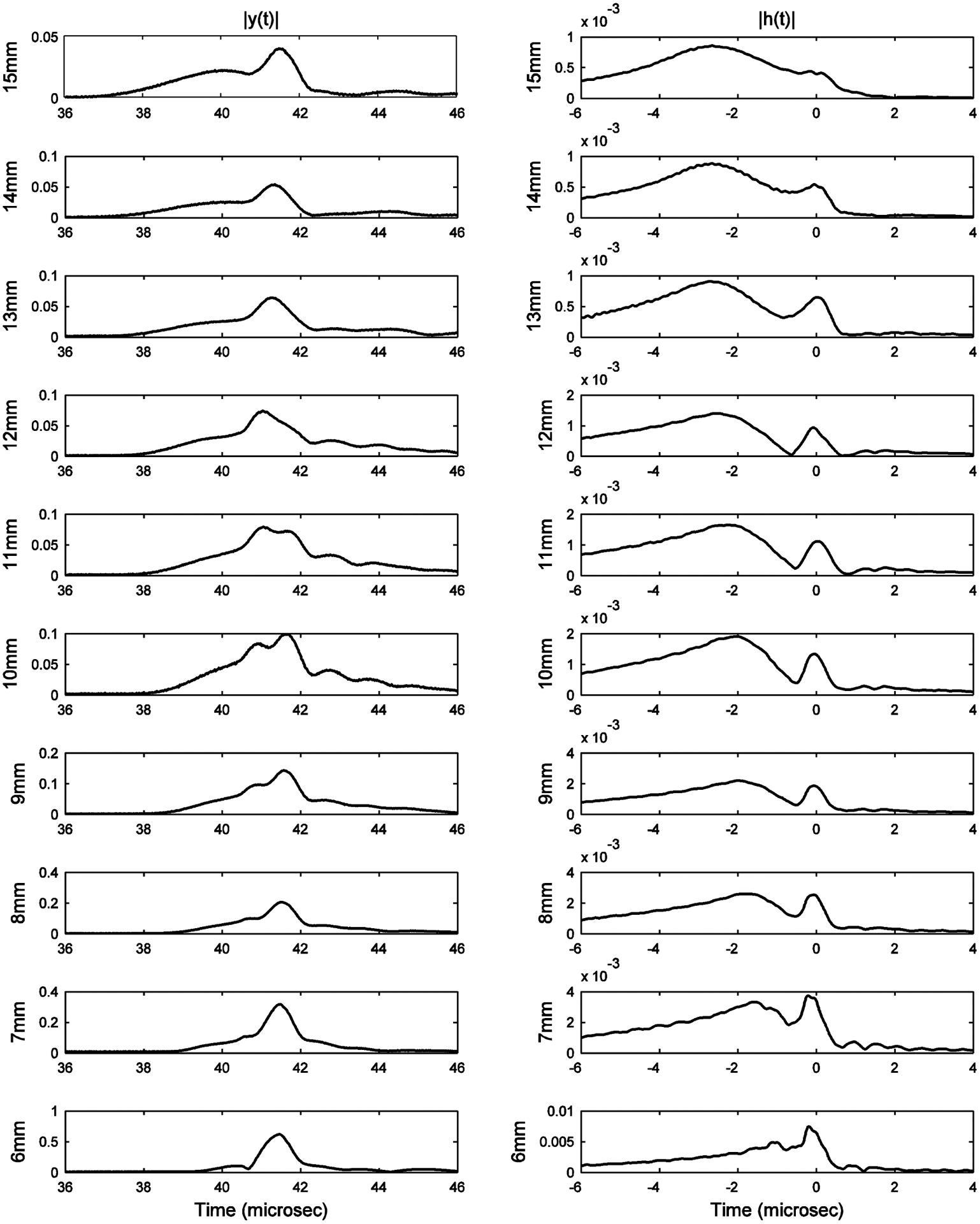
Envelopes of radio-frequency signals (left column) and deconvolved signals (right column) transmitted through bovine cancellous bone for thicknesses ranging from 6 to 15 mm. Data are auto-scaled in order to show maximum detail for each signal.
Based on Figure 5, it was determined that good separation between fast and slow waves existed for thicknesses ranging from 7 to 12 mm. Therefore, in this paper, measurements of fast and slow wave properties are reported in the range from 7 to 12 mm.
B. |Htotal(f)|, |Hfast(f)|, and |Hslow(f)|
Figure 6 shows |Htotal(f)|, |Hfast(f)|, and |Hslow(f)| for the bone sample with thickness equal to 9 mm. Hfast(f) and Hslow(f) were obtained by 1) inverse FFT of the measurement of Htotal(f), 2) time domain separation of hfast(t) from hslow(t) at the time shift of the local minimum in the envelope of htotal(t) between time shifts corresponding to velocities between 1550 and 1700 m/s, and 3) FFT of hfast(t) and hslow(t). It can be seen that Htotal(f), which has a complicated frequency dependence, can be decomposed into two component filter functions, Hfast(f) and Hslow(f), with quasi-linear frequency dependence, as shown previously (Wear, 2014).
Figure 6.

|Htotal(f)|, |Hfast(f)|, and |Hslow(f)| for the bone sample with thickness equal to 9 mm.
A correlation coefficient for Hfast(f) vs. f or Hslow(f) vs. f near one can be taken to be an indication of successful isolation of a single mode wave (fast or slow) (Haiat et al., 2008). The correlation coefficients were 0.997 ± 0.002 and 0.986 ± 0.013 for fast and slow waves respectively (mean ± standard deviation). These consistently high correlation coefficients support 1) the decomposition of the signal into two waves with linear-with-frequency attenuation, and 2) successful fast and slow wave isolation with bandlimited deconvolution.
C. Fast and Slow Wave Properties as Functions of Thickness
Figure 7 shows signal velocity versus thickness for the bone sample. Signal velocity is associated with the fast wave.
Figure 7.

Signal velocity vs. thickness for the bone sample. Error bars denote standard errors.
Figure 8 shows measurements of phase velocity and signal loss as functions of bone sample thickness for fast (left column) and slow (right column) waves. Figure 8 suggests that fast wave phase velocity at 350 kHz increased with thickness while slow wave phase velocity at 750 kHz decreased with thickness (top row). Signal loss tended to increase with bone thickness for fast and slow waves, which is expected since signal loss is not normalized to bone thickness.
Figure 8.

Measurements of phase velocity and signal loss as functions of bone sample thickness for fast and slow waves.
Previously, Nelson et al. (2011) reported Bayesian-method-based measurements of fast and slow wave parameters at one thickness value (9 mm) for one of the bone samples investigated in the present study. Table I shows a comparison of fast and slow wave parameters measured in the two studies. Values reported by Nelson et al. at 1 MHz were converted to 350 kHz and 750 kHz using Equation 3. The two studies are in fairly good agreement, considering the complexity of the signals.
Table I.
Comparison of parameter values obtained using three algorithms: Bayesian (Nelson et al., 2011), Deconvolution, and MLSP+CF on bone sample with thickness of 9 mm from Nagatani et al. (2008).
| Parameter | wave | Frequency (kHz) | Bayesian | Deconvolution | MLSP+CF |
|---|---|---|---|---|---|
| Signal Loss (dB) | fast | 350 | 15.5 | 16.7 | 18.6 |
| slow | 750 | 22.5 | 23.1 | 23.6 | |
| Phase Velocity (m/s) | Fast | 350 | 1731 | 1717 | 1683 |
| slow | 750 | 1470 | 1462 | 1470 |
Average root-mean-squared (RMS) differences between the bandlimited deconvolution and MLSP+CF for phase velocities were 5 m/s (fast wave, 350 kHz) and 13 m/s (slow wave, 750 kHz). Average RMS differences for signal loss at 500 kHz were 1.6 dB/cmMHz (fast wave) and 0.4 dB/cmMHz (slow wave).
The average computation time for deconvolution was less than half of one second. The average computation time for MLSP+CF was 3.3 sec. Data analysis was performed using a Dell notebook computer with Intel® Core™ i5-2520M CPU @ 2.5 GHz with 4 GB RAM.
DISCUSSION
In this study, phase velocity and attenuation for fast and slow waves were measured in bovine cancellous bone samples as functions of bone sample thickness. Two algorithms were used to separate fast and slow waves: bandlimited deconvolution and MLSP+CF. Bandlimited deconvolution consistently decomposed signals into two waves with linear attenuation, as evidenced by very high correlation coefficients (mean r > 0.98) between fast or slow wave attenuation coefficient and frequency. This finding supports the model for two linearly-attenuating waves in cancellous bone originally proposed by Marutyan et al. (2006). In addition, this finding supports the ability of bandlimited deconvolution to successfully isolate those linearly-attenuating fast and slow waves. The model is useful because it reduces the data reduction task to a manageable number of parameters (six) and does not require extensive knowledge of the material and structural properties of the bone in order to estimate those parameters. The true physics underlying fast and slow wave propagation is probably more complicated than the model indicates. Other approaches may offer more realistic analysis of the interaction between ultrasound and bone (Hosokawa and Otani, 1997; Haire and Langton, 1999; Kaczmarek et al., 2002; Lee et al., 2003; Fellah et al., 2004; Meziere et al., 2013). Nevertheless, the two linearly-attenuated wave model has been shown to be very effective in investigations of cancellous bone (Marutyan et al., 2006; Marutyan et al., 2007; Anderson et al., 2008; Anderson et al., 2010; Nelson et al., 2011; Hoffman et al., 2012).
A simulation was performed, using previous methods (Wear, 2014), in order to investigate whether the potential trends of phase velocity vs. bone thickness shown in Figure 8 could be artifacts of the estimation algorithms. For example, as shown in Figure 5, even after deconvolution, there remains some overlap between fast and slow waves. This overlap could degrade the accuracy of phase velocity estimates. The simulation assumed constant values for phase velocity and attenuation parameters reported by Nelson et al. (2011) at 1 MHz, which were converted to 350 kHz (fast wave) and 750 kHz (slow wave) using Equation 3. The signal-to-noise ratio (SNR) was assumed to be 51 dB, which was the average level measured for the current data set. As shown in Figure 9, the simulation did not show a significant thickness-dependent bias of estimates of phase velocity. Nelson et al. (2011) performed a similar simulation check on their Bayesian algorithm, showing that it did not introduce a thickness-dependent bias on attenuation coefficient at 1 MHz (Nelson et al., 2011, Figure 4). Note that while Nagatani et al. (2008) and Nelson et al. (2011) plotted attenuation of 1 mm slabs, Figures 8 and 9 show properties for entire bone samples. Therefore, while attenuation coefficient at 1 MHz in Figure 4 from Nelson et al. (2008) remained constant with sample thickness, signal loss in Figure 9 from the present paper increased with sample thickness.
Figure 9.

Simulation results for estimated phase velocity and signal loss as functions of bone thickness, assuming constant phase velocity and attenuation parameters from Nelson et al. (2011). The standard deviations for phase velocity estimates are less than 1 m/s. The standard deviations for signal loss estimates are less than 0.04 dB. The dashed lines show the true values for the parameters.
As mentioned above, the correlation coefficients between fast and slow wave attenuation coefficients and frequency were high: 0.997 ± 0.002 (fast wave) and 0.986 ± 0.013 (slow wave) (mean ± standard deviation). This consistently high value supports 1) the decomposition of the signal into two waves with linear-with-frequency attenuation, and 2) successful fast and slow wave isolation with bandlimited deconvolution. In addition, similar trends were measured using two different algorithms (bandlimited deconvolution and MLSP+CF) even though they had considerably different sources of estimation error (discussed below).
Other factors that could have contributed to the observed trends are 1) diffraction errors, which were not perfectly eliminated in the substitution experiments because the wavelengths of ultrasound are different in bone than in water, and 2) inhomogeneity of the sample. Analysis of data from additional bone samples will be required in order to resolve the significance of the changes in measurements of vfast(350 kHz) with thickness observed in the present study.
Average root-mean-squared (RMS) differences between the bandlimited deconvolution and MLSP+CF for phase velocities were 5 m/s (fast wave, 350 kHz) and 13 m/s (slow wave, 750 kHz). Average RMS differences for signal loss at 500 kHz were 1.6 dB/cmMHz (fast wave) and 0.4 dB/cmMHz (slow wave). Quantitative disparities between bandlimited deconvolution and MLSP+CF may arise because the two algorithms rely on different assumptions and have different error sources. For example, bandlimited deconvolution applies filters and a window to H(f) in frequency domain that can produce distortion in h(t), which is calculated as the inverse FFT of H(f). In addition, bandlimited deconvolution imposes a time threshold that divides the deconvolved time domain signal, h(t), into fast and slow components, while in reality fast and slow waves can overlap and therefore leak beyond the designated threshold (Wear, 2014). MLSP+CF imposes a relationship between attenuation slope and dispersion (Equation 3), but errors in the attenuation model (e.g., slight deviations from linear-with-frequency attenuation) would lead to errors in the dispersion model. In addition, MLSP+CF assumes that the MLSP method (Wear, 2010) applied in the first stage provides good initial guesses for parameter values and that the parameter search spaces it uses in the second and third stages include the correct parameter combination (Wear, 2013). Despite these disparate sources of error, the two methods agreed fairly well.
Sources for disagreement among the analysis methods considered here (bandlimited deconvolution and MLSP+CF) and a Bayesian method (Nelson et al., 2011) include different pre-processing (in the present study: multi-path filter, interpolation, and bandpass filtering), different frequency bands of analysis, and different underlying assumptions of the methods. Limitations of bandlimited deconvolution and MLSP+CF were discussed above. One assumption in the Bayesian method that is not made in bandlimited deconvolution or MLSP+CF is that the fast and slow wave phase velocities and attenuation slopes are independent of each other so that their joint probability density function may be factored into the product of four univariate probability density functions (Marutyan et al., 2007, Equation 4).
The disparities between bandlimited deconvolution and MLSP+CF should be considered in the context of limitations of accuracy and precision due to experimental error. For example, estimates of mean phase cancellation errors in measurements of attenuation parameters in cancellous bone range have been reported to be 2.5 – 8.3 dB/cmMHz (attenuation slope) in vitro (Wear, 2008; Cheng et al., 2011) and 14.2 dB/MHz (broadband ultrasound attenuation) in vivo (Wear, 2007). In addition, imperfect diffraction compensation can arise in substitution experiments due to velocity mismatch between sample and reference (water) (Xu and Kaufman, 1993; Kaufman et al., 1995; Droin et al., 1998). This effect is more severe for the fast wave. Droin et al. (1998) showed that between 200 and 800 kHz, a velocity mismatch of approximately 720 m/s can result in errors on the order of −0.4 dB/cm for attenuation and −20 m/s for phase velocity. Other sources of experimental error include refraction artifacts, multipath interference, and non-normal incidence.
CONCLUSION
Bandlimited deconvolution and MLSP+CF are fast signal-processing methods that showed reasonable agreement with each other and with a Bayesian method for measurements of fast and slow wave phase velocities and signal loss in bovine cancellous bone. Bandlimited deconvolution consistently decomposed signals into two waves with linear attenuation, as evidenced by very high correlation coefficients between fast and slow wave attenuation coefficients and frequency. This finding supports the model for two linearly-attenuating longitudinal waves for bovine cancellous bone when ultrasound propagates parallel to the predominant trabecular orientation.
ACKNOWLEDGEMENTS
Part of this work was supported by the Regional Innovation Strategy Support Program of Ministry of Education, Culture, Sports, Science and JSPS KAKENHI Grant Number 24360161 and 25871038.
REFERENCES
- Anderson CC, Bauer A,Q, Holland MR, Pakula M, Laugier P, Bretthorst G,L, and Miller J,G, (2010), “Inverse problems in cancellous bone: estimation of the ultrasonic properties of fast and slow waves using Bayesian probability theory,” 128, 2940–2948. [DOI] [PMC free article] [PubMed] [Google Scholar]
- Breban S, Padilla F, Fujisawa Y, Mano I, Masukawa M, Benhamou CL, Otani T, Laugier P, and Chappard C, (2010). “Trabecular and cortical bone separately assessed at radius with a new ultrasound device, in a young adult population with various physical activities,” Bone, 46, 1620–1625. [DOI] [PubMed] [Google Scholar]
- Cardoso L, Teboul F, Sedel L, Oddou C, and Meunier A, (2003). “In vitro acoustic waves propagation in human and bovine cancellous bone,” J. Bone. Miner. Res, 18, 1803–1812. [DOI] [PubMed] [Google Scholar]
- Cheng J, Serra-Hsu FS, Tian Y, Lin W, and Qin YX,(2011) “Effects of phase cancellation and receiver aperture size on broadband ultrasonic attenuation for trabecular bone in vitro,” Ultrasound in Med., & Biol, 37, 2116–2125. [DOI] [PMC free article] [PubMed] [Google Scholar]
- Dencks S, Barkmann R, Gluer CC, and Schmitz G, (2009) “Model-based parameter estimation in the frequency domain for quantitative ultrasound measurement of bone,” Proc. IEEE Ultrasonics Symp, 554–557. [Google Scholar]
- Dencks S, Schmitz G, (2013), “Estimation of multipath transmission parameters for quantitative ultrasound measurements of bone,” IEEE Trans. Ultrason. Ferro., and Freq. Cont, 60, 1884–1895. [DOI] [PubMed] [Google Scholar]
- Droin P, Berger G and Laugier P, (1998). “Velocity dispersion of acoustic waves in cancellous bone.” IEEE Trans. Ultrason. Ferro. Freq. Cont 45, 581–592. [DOI] [PubMed] [Google Scholar]
- Fellah ZEA, Chapelon JY, Berger S, Lauriks W, and Depollier C, (2004). “Ultrasonic wave propagation in human cancellous bone: application of Biot theory, J. Acoust. Soc. Am, 116, 61–73. [DOI] [PubMed] [Google Scholar]
- Fujita F, Mizuno K, and Matsukawa M, (2013). “An experimental study on the ultrasonic wave propagation in cancellous bone: Waveform changes during propagation.” J. Acoust. Soc. Am, 134, 4775–4781. [DOI] [PubMed] [Google Scholar]
- Haïat G, Padilla F, Peyrin F, and Laugier P, (2008). “Fast wave ultrasonic propagation in trabecular bone: numerical study of the influence of porosity and structural anisotropy,” J. Acoust. Soc. Am, 123, 1694–1705. [DOI] [PubMed] [Google Scholar]
- Haire TJ, and Langton CM, (1999). “Biot theory: a review of its application to ultrasound propagation through cancellous bone,” Bone, 24, 291–295. [DOI] [PubMed] [Google Scholar]
- Hoffman JJ, Nelson AM, Holland MR, and Miller JG, (2012). “Cancellous bone fast and slow waves obtained with Bayesian probability theory correlate with porosity from computed tomography,” J. Acoust. Soc. Am, 132, 1830–1837. [DOI] [PMC free article] [PubMed] [Google Scholar]
- Hosokawa A, and Otani T, (1997). “Ultrasonic wave propagation in bovine cancellous bone,” J. Acoust. Soc. Am, 101, 558–562. [DOI] [PubMed] [Google Scholar]
- Hosokawa A, and Otani T, (1998). “Acoustic anisotropy in bovine cancellous bone,” J. Acoust. Soc. Am, 103, 2718–2722. [DOI] [PubMed] [Google Scholar]
- Kazmarek M, Kubik J, and Pakula M, (2002). “Short ultrasonic waves in cancellous bone,” Ultrasonics, 40, 95–100. [DOI] [PubMed] [Google Scholar]
- Kaufman JJ, Xu W, Chiabrera AE, and Siffert RS (1995), “Diffraction effects in insertion mode estimation of ultrasonic group velocity,” IEEE Trans. Ultrason. Ferro., Freq. Cont, 42, 232–242. [Google Scholar]
- Lashkari B, Manbachi A, Mandelis A, and Cobbold RSC (2012). “Slow and fast ultrasonic wave detection improvement in human trabecular bones using Golay code modulation,” J. Acoust. Soc. Am, 132, (3), EL222–EL228. [DOI] [PubMed] [Google Scholar]
- Laugier P, (2011), “Quantitative Ultrasound Instrumentation for Bone In Vivo Characterization” in Bone Quantitative Ultrasound, ed. Laugier P and Haiat G, Springer, New York, NY., chapter 3, 47–72. [Google Scholar]
- Lee KI, Roh H, and Yoon SW (2003), “Acoustic wave propagation in bovine cancellous bone: Application of the modified Biot-Attenborough model,” J. Acoust. Soc. Am, 114, 2284–2293. [DOI] [PubMed] [Google Scholar]
- Lin L, Cheng J, Lin W, and Qin Y-X, (2012), “Prediction of trabecular bone principal structural orientation using quantitative ultrasound scanning,” J. Biomech, 45, 1790–1795. [DOI] [PMC free article] [PubMed] [Google Scholar]
- Mano I, Horii K, Takai S, Suzaki T, Nagaoka H, and Otani T, (2006), “Development of novel ultrasonic bone densitometry using acustic parameters of cancellous bone for fast and slow waves,” Jap. J. Appl. Phys, 45, 4700–4702. [Google Scholar]
- Mano I, Yamamoto T, Hagino H, Teshima R, Takada M, Tsujimoto T, and Otani T, (2007), “Ultrasonic transmission characteristics of in vitro human cancellous bone,” Jap. J. Appl. Phys, 46, 4858–4861. [Google Scholar]
- Maruo S, and Hosokawa A, (2014), “A generalized harmonic analysis of ultrasound waves propagating in cancellous bone,” Japanese J. Appl. Phys, 53, 07KF06 [Google Scholar]
- Marutyan KR, Holland MR, and Miller JG (2006), “Anomalous negative dispersion in bone can result from the interference of fast and slow waves,” J. Acoust. Soc. Am, 120, EL55–EL61. [DOI] [PubMed] [Google Scholar]
- Marutyan KR, Bretthorst GL, and Miller JG (2007). “Bayesian estimation of the underlying bone properties from mixed fast and slow mode ultrasonic signals” J. Acoust. Soc. Am, 121, EL8–EL15. [DOI] [PubMed] [Google Scholar]
- Meziere F, Muller M, Bossy E, and Derode A, (2014), “Measurements of ultrasound velocity and attenuation in numerical anisotropic porous media compared to Biot’s and multiple scattering models,” Ultrasonics, 54, 1146–1154. [DOI] [PubMed] [Google Scholar]
- Mizuno K, Matsukawa M, Otani T, Takada M, Mano I, Tsujimoto T, (2008), “Effects of structural anisotropy of cancellous bone on speed of ultrasonic fast waves in the bovine femur,” IEEE Trans. Ultrason., Ferroelec., and Freq. Contr, 1480–1487. [DOI] [PubMed] [Google Scholar]
- Mizuno K, Somiya H, Kubo T, Matsukawa M, Otani T, and Tsujimoto T, (2010), “Influence of cancellous bone microstructure on two ultrasonic wave propagations in bovine femur: an in vitro study,” J. Acoust. Soc. Am, 128, 3181–3189. [DOI] [PubMed] [Google Scholar]
- Mizuno K, Nagatani Y, Yamashita K, and Matsukawa M, (2011), “Propagation of two longitudinal waves in a cancellous bone with a closed pore boundary,” J. Acoust. Soc. Am, 130, EL122 – EL127. [DOI] [PubMed] [Google Scholar]
- Nagatani Y, Mizuno K, Saeki T, Matsukawa M, Sakaguchi T, and Hosoi H, (2008), “Numerical and experimental study on the wave attenuation in bone – FDTD simulation of ultrasound propagation in cancellous bone,” Ultrasonics, 48, 607–612. [DOI] [PubMed] [Google Scholar]
- Nagatani Y, Mizuno K, and Matsukawa M, (2014), “Two-wave behavior under various conditions of transitional area from cancellous bone to cortical bone,” Ultrasonics, 54, 1245–1250. [DOI] [PubMed] [Google Scholar]
- Nagatani Y, and Tachibana RO (2014), “Multichannel instantaneous frequency analysis of ultrasound propagating in cancellous bone,” J. Acoust. Soc. Am, 135, 1197–1206. [DOI] [PubMed] [Google Scholar]
- Nelson AM, Hoffman JJ, Anderson CC, Holland MR, Nagatani Y, Mizuno K, Matsukawa M, and Miller JG, (2011), “Determining attenuation properties of interfering fast and slow ultrasonic waves in cancellous bone,” 130, 2233–2240. [DOI] [PMC free article] [PubMed] [Google Scholar]
- O’Donnell M, Jaynes ET, and Miller JG, (1981) “Kramers-Kronig relationship between ultrasonic attenuation and pahse velocity,” J. Acoust. Soc. Am, 69, 696–701. [Google Scholar]
- Oppenheim AV, and Schafer RW, (1975), Digital Signal Processing, (Prentice-Hall Inc., Englewood Cliffs, NJ: ), Chap. 5, p. 243. [Google Scholar]
- Otani T, (2005), “Quantitative estimation of bone density and bone quality using acoustic parameters of cancellous bone for fast and slow waves,” Jap. J. Appl. Phys, 44, 4578–4582. [Google Scholar]
- Otani T, Mano I, Tsujimoto T, Yamamoto T, Teshima R, and Naka H, (2009), “Estimation of in vivo cancellous bone elasticity,” Jap. J. Appl. Phys, 48, 07GK05–1–07GK05–5. [Google Scholar]
- Sai H, Iguchi G, Tobimatsu T, Takahashi K, Otani T, Horii K, Mano I, Nagai I, Iio H, Fujita T, Yoh K, and Baba H, (2010) “Novel ultrasonic bone densitometry based on two longitudinal waves: significant correlation with pQCT measurement values and age-related changes in trabecular bone density, cortical thickness, and elastic modulus of trabecular bone in a normal Japanese population,” Osteo. Int, 21, 1781–1790. [DOI] [PubMed] [Google Scholar]
- Waters KR and Hoffmeister BK, (2005). “Kramers-Kronig analysis of attenuation and dispersion in trabecular bone,” J Acoust Soc Am, 118,3912–3920. [DOI] [PubMed] [Google Scholar]
- Wear KA (2000a), “Measurements of phase velocity and group velocity in human calcaneus,” Ultrason. Med. Biol, 26, 641–646. [DOI] [PMC free article] [PubMed] [Google Scholar]
- Wear KA (2000b), “The effects of frequency-dependent attenuation and dispersion on sound speed measurements: applications in human trabecular bone,” IEEE Trans. Ultrason., Ferro., and Freq. Cont, 47, 265–273. [DOI] [PMC free article] [PubMed] [Google Scholar]
- Wear KA, (2007), “The effect of phase cancellation on estimates of calcaneal broadband ultrasound attenuation in vivo,” IEEE Trans Ultrason., Ferro., and Freq. Cont, 54, 1352–1359. [DOI] [PMC free article] [PubMed] [Google Scholar]
- Wear KA, (2008), “The effect of phase cancellation on estimates of broadband ultrasound attenuation and backscatter coefficient in human calcaneus in vitro,” IEEE Trans Ultrason., Ferro, and Freq. Cont, 55, 384–390. [DOI] [PMC free article] [PubMed] [Google Scholar]
- Wear KA, (2010), “Decomposition of two-component ultrasound pulses in cancellous bone using modified least squares Prony’s method—phantom experiment and simulation,” Ultrasound Med. & Biol, 36, 276–287. [DOI] [PMC free article] [PubMed] [Google Scholar]
- Wear KA, (2013), “Estimation of fast and slow wave properties in cancellous bone using Prony’s method and curve fitting,” J. Acoust. Soc. Am, 133, 2490–2501. [DOI] [PMC free article] [PubMed] [Google Scholar]
- Wear KA, (2014), “Time-domain separation of interfering waves in cancellous bone using bandlimited deconvolution: simulation and phantom study. J. Acoust. Soc. Am, 135, 2102–2112. [DOI] [PMC free article] [PubMed] [Google Scholar]
- Xu W, Kaufman JJ, (1993). “Diffraction correction methods for insertion ultrasound attenuation estimation,” IEEE Trans Biomed. Eng, 40, 563–569. [DOI] [PubMed] [Google Scholar]
- Yamashita K, Fugita F, Mizuno K, Mano I, Matsukawa M, (2012), “Two-wave propagation imaging to evaluate the structure of cancellous bone,” IEEE Trans. Ultrason., Ferro., Freq. Cont, 59, 1160–1166. [DOI] [PubMed] [Google Scholar]