The Effect of Social Distancing on the Early Spread of the Novel Coronavirus

Abstract

This article quantifies the effect of individual social distancing on the spread of the novel coronavirus. To do so, we use data on time spent by individuals on activities that would potentially expose them to crowds from the American Time Use Survey linked with state‐level data on positive tests from the COVID Tracking Project. We estimate count data specifications of observed COVID‐19 infections at the state level as a function of control demographic variables, and a measure of social distance that captures the amount of time individuals across the states spend in activities that potentially expose them to crowds. Parameter estimates reveal that the number of state‐level novel coronavirus infections decrease with respect to our measure of individual social distance. From a practical perspective, our parameter estimates suggest that if the typical individual in a U.S. state were to spend eight hours away from crowds completely, this would translate into approximately 240,000 fewer COVID‐19 infections across the states. Our results suggest that, at least in the United States, social distancing policies are effective in slowing the spread of the novel coronavirus.

The first known case of the novel coronavirus (COVID‐19) was detected in the city of Wuhan, China on December 31, 2019 (Khan and Atangana, 2020). Since that time, it has emerged as a global pandemic, with the first recorded infection in the United States occurring on January 21, 2020 (Holshue et al., 2020).

The number of cases increased slowly in the United States during the early months of 2020, only reaching 88 by March 1. From that date cases grew exponentially, increasing by a power of roughly 2.58, as shown in Figure 1. While the dramatic rise in cases also represents the increase in attention and testing capacity, the steep trend demonstrates the rapid expansion of the scope of the crises.

FIGURE 1.

Confirmed COVID‐19 Cases Over Time

As a result, state governments began to take action in order to slow the spread of the virus. Washington was the first state to declare a state of emergency on February 29, but every state had done so before the end of March. The apparent success of encouraging individuals to avoid large crowds—social distancing—during the 1918–1919 Spanish Flu pandemic (Markel et al., 2007; Smith, 2007) and 2009 global influenza pandemic (Bajardi et al., 2011) led many political jurisdictions in the United States to recommend and implement social distancing policies (Bedford et al., 2020) to slow the spread of COVID‐19 infections in the population. To the extent that the spread of COVID‐19 is similar to influenza with respect to its airborne transmission via expelled aerosols and droplets by COVID‐19 infected individuals, social distancing by individuals can plausibly slow the spread of COVID‐19.

In this article, we attempt to quantify the effects of social distancing on the early spread of the novel coronavirus with data on individual time spent in crowds from the American Time Use Survey (ATUS) linked with state‐level data on positive tests from the COVID Tracking Project. In contrast to the recent approach of Fang, Wang, and Yang (2020), which utilizes aggregate human mobility reductions to infer the effects of social distance on the spread COVID‐19 in China, our approach utilizes individual time spent in specific activities that can expose them to crowds to infer the effects of social distance on the spread of COVID‐19 in the United States.

Our inquiry contributes to a growing body of research on determinants of COVID‐19's spread. For instance, Courtemanche et al. (2020) found that the earlier enactment of social distancing measures reduced the spread of the disease in March and April. Using a similar event‐study methodology, Abouk and Heydari (2021) found that stay‐at‐home orders were the most effective form of social distancing being used in the United States across states. In addition, Wang et al. (2020) found that social distancing was required to prevent hospital overload, specifically in Texas—though other states likely faced similar predicaments. However, rather than looking at the impact of specific policies, our article analyzes how preexisting levels of social distancing impacted the initial spread of COVID‐19 as one of the determinants of early outbreaks of the disease.

Beyond policy and social distancing, other sociodemographic determinants have been shown to be associated with the spread of COVID‐19. For instance, older individuals have faced a disproportionate number of severe cases from COVID‐19, particularly those living in nursing homes. In addition, preexisting health conditions such as heart disease and diabetes have been shown to increase the chances of contracting COVID‐19 (Caramelo, Ferreira, and Oliveiros, 2020). Less causally, certain community demographics have been associated with worse outbreaks; in particular, minorities and lower socioeconomic status communities have had worse outbreaks as a result of structural inequalities, labor force practices, and access to health care (Adhikari et al., 2020; van Holm, Wyczalkowski, and Dantzler, 2020; Wadhera et al., 2020). As such, along with social distancing other factors must be accounted for in predicting the level of outbreak in any state.

The remainder of this article is organized as follows. In the second section, we discuss the data and methodology of the study. Our individual COVID‐19 infection data are at the U.S. state‐level between March 3, 2020 and March 27, 2020. We link these data with measures of aggregate individual time use in activities that could expose individuals to crowds from 2018 American Time Use Data. The third section reports parameter estimates from count data specifications of individual COVID‐19 infections at the state level as a function of our measure of social distancing, community demographics, and the local economy. The last section concludes with a discussion of the implications of the research for the efficacy of social distance policies as a tool to slow the spread of COVID‐19.

Data and Methodology

The data for our study comes from three sources. Data on the number of COVID‐19 infections at the state level are from the COVID Tracking Project. We accessed the data on March 28, 2020 at 1:58PM EDT. For each state in the United States, and for the time period March 3, 2020 and March 27, 2020, the COVID Tracking Project data provides counts on the number of individual positive tests for COVID‐19.1 For our analysis, we construct a panel across time for all 50 U.S. states and the District of Columbia, and exclusive of U.S. territories and Puerto Rico.

The 2018 ATUS (Hofferth et al., 2020) is the source of the data upon which we construct our social distance measure.2 We construct a measure of social distance from the 2018 ATUS based upon the number of minutes over a 24‐hour period that individuals report spending on activities that could potentially expose them to crowds. Table 1 reports on the particular questions from the ATUS we determined are activities that could potentially expose individuals to crowds.

TABLE 1.

Description of ATUS Time Activity Measures

Activity Variable: Minutes Spent Doing	Definition
BLS PCARE TRAVEL BLS	Travel related to personal care
FOOD TRAVEL BLS	Travel related to eating and drinking
HHACT TRAVEL BLS	Travel related to household activities
PURCH TRAVEL BLS	Travel related to purchasing goods and services
CAREHH TRAVEL BLS	Travel related to caring for and helping household members
CARENHH TRAVEL BLS	Travel related to caring for and helping non‐household members
WORK TRAVEL BLS EDUC	Travel related to work
TRAVEL BLS SOCIAL	Travel related to education
TRAVEL BLS COMM	Travel related to organizational, civic, and religious activities
TRAVEL BLS LEIS TRAVEL	Travel related to telephone calls
BLS LEIS ARTS	Travel related to leisure and sports
–	Leisure and sports: Arts and entertainment (other than sports)
BLS LEIS PARTSPORT	Participating in sports, exercise, and recreation
BLS LEIS ATTSPORT BLS	Attending sporting or recreational events
LEIS ATTEND BLS LEIS	Attending or hosting social events
SOCCOM BLS LEIS	Socializing and communicating
SOCCOMEX BLS PURCH	Socializing and communicating (except social events)
GOV BLS PURCH GROC	Purchasing goods and services: Government services
BLS PURCH CONS BLS	Purchasing goods and services: Grocery shopping
PURCH VEHIC BLS	Purchasing goods and services: Consumer goods purchases
PURCH PROF BLS	Purchasing goods and services: Vehicle maintenance and repair services (not done by self)
PURCH BANK BLS	Purchasing goods and services: Professional and personal care services
PURCH HEALTH BLS	Purchasing goods and services: Financial services and banking
PURCH HHSERV BLS	Purchasing goods and services: Medical and care services
PURCH HOME	Purchasing goods and services: Household services
–	Purchasing goods and services: Home maintenance, repair, decoration, and construction (not done by self)
BLS SOCIAL CULTURE	Participating in performance and cultural activities
BLS SOCIAL ADMIN BLS	Organizational, civic, and religious activities: Administrative and support activities
SOCIAL ATTEND BLS	Attending meetings, conferences, and training
SOCIAL CIVIC BLS	Civic obligations and participation
SOCIAL MAINTEN	Organizational, civic, and religious activities: Indoor and outdoor maintenance, building, and cleanup activities
BLS SOCIAL SOCSERV	Organizational, civic, and religious activities: Social service and care activities (except medical)
BLS SOCIAL VOL BLS	Organizational, civic, and religious activities: Volunteering (organizational and civic activities)
SOCIAL VOLACT BLS	Organizational, civic, and religious activities: Volunteer activities Attending class
EDUC CLASS BLS WORK SEARCH	Working and work‐related activities: Job search and interviewing

Source: 2018 IPUMS American Time Use Survey.

Each of the 2018 ATUS time use questions are mutually exclusive, and respondents report minutes spent on the activity over a 24‐hour period. For each respondent, the sum of the answers to the questions in Table 1 was subtracted from the total number of minutes in a day (1,440). This difference is our measure of social distance for each respondent in the 2018 ATUS; it is our measure of the total time in minutes spent in activities not potentially exposed to large crowds. As shown in Figure 2, there is substantial variation between states in the average social distancing of citizens, with no regional patterns discernable.

FIGURE 2.

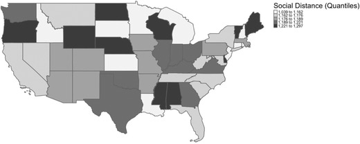
Social Distancing Across Continental States

The social distance measure was estimated for the typical individual in each U.S. state by computing the weighted mean.3 In this context, our analysis assumes individual choices about allocating time across various activities can be captured by a representative agent at the state level, measured by the state‐level mean of our social distance measure. While representative agent approaches can fail in capturing important sources of heterogeneity among individuals Barker and de‐Ramon (2006), they can also closely correspond with the behavior of heterogeneous agents (Phillips, 2019)—property we have to exploit giving the necessity of linking state‐level counts on COVID‐19 infections with individual behavioral data.

As our dependent variable is integer‐valued, our parameter estimates of the effects of social distancing on state‐level COVID‐19 infections are based upon count data estimator specifications. Suppose C_it the number of COVID‐19 infections in state i at time t is distributed as a Poisson or negative binomial random variable with mean λ_it . For C_it = c = 0, 1, . . . N, the respective Poisson and negative binomial densities are:

$$\mathrm{Prob}(C_{it}=c)=e^{-\lambda it}{{\lambda }_{it}}^c/c!$$ (1)

$$\mathrm{Prob}(C_{it}=c)=[\mathrm{\Gamma }(c+1/\alpha )/\mathrm{\Gamma }(1/\alpha )c!]\times {{[(1/\alpha )/1/\alpha +{\lambda }_{it}]}^1}^{/\alpha }\times {[{\lambda }_{it}/1/\alpha +{\lambda }_{it}]}^c$$ (2)

where λ_it = exp(β_iX_it ), X_it is the ith covariate at time t that explains the mean value λ_it , β_i is the effect of X_it on λ_it , Γ is the Gamma distribution, and α is a dispersion parameter.

Pooling observations across the time periods under consideration, log‐likelihood regression specifications of (1) and (2) permit Poisson and negative binomial parameter estimates, respectively, of how particular covariates X_it effect the number of COVID‐19 infections in state i and time t. Our dependent variable C_it is the number of COVID‐19 infections.

As control covariates to mitigate the effects of confounding, we include 13 variables to account for state demographics and the labor force. Data on demographics and the labor force were collected from the Integrated Public Use Microdata Series (IPUMS) using the 2018 1‐year American Community Survey. Specifically, we control for the percentage of the state population that is African American, percentage of the state that is Latinx, percentage of state population that is foreign born, average age of individuals in state, percentage of state population with a baccalaureate degree, percentage of state population that is self‐employed, percentage of state population that lives in metropolitan areas, and the average weekly earnings in the state. In addition, the model accounts for the impact of the labor force and the ways that different industries were potentially exposed to COVID‐19 early in the pandemic. Specifically, we include a measure for the percentage of the labor force that works in accommodations or entertainment, the percentage that works in healthcare, and the percentage that works in retail. All three aspects of the labor force should positively predict the number of COVID‐19 cases.

Results

Table 2 reports a statistical summary of all covariates constructed in our data to estimate the count data regression specifications.4 In Table 3, we report time fixed effect parameter estimates for Poisson and negative binomial regression specifications of the number of COVID‐19 infections at the state level. The fixed effect parameter estimates reported in Table 3 condition any unobservables explicitly on time, mitigating or eliminating any bias in parameter estimates due to unobserved heterogeneity across the states that is a function of the time path of COVID‐19 infections.

TABLE 2.

Summary Statistics

Variable	Mean	Std. Dev.	Min	Max
Number of positive cases	394.1799	2311.144	0	44635
Mean social distance of individuals in state (minutes per day)	1185.582	46.24771	1039.117	1296.798
Percentage of males	0.493567	0.007911	0.476005	0.517365
Percentage of African Americans	0.111705	0.104	0.005927	0.44239
Percentage of Latino/Latina/Latinx	0.123938	0.103858	0.01469	0.492641
Percentage of state with bachelor's degree or higher	0.344235	0.069243	0.226414	0.632259
Percentage of labor force employed	0.111618	0.02018	0.077688	0.175108
Percentage of Individuals with home access to Internet	0.809559	0.035006	0.699197	0.882497
Percentage of residents living inside MSA	0.681507	0.246464	0	1
Median age of residents	43.33013	3.235945	33	51
Population of state (100,000)	66.45874	74.56481	5.78759	395.1222
Median Income of state ($10,000)	7.850979	1.443466	5.76	11.31
Percentage of labor force in accommodations	0.122674	0.024266	0.092992	0.263641
Percentage of labor force in healthcare	0.159797	0.020622	0.104825	0.20107
Percentage of labor force in retail	0.132103	0.014897	0.060642	0.160024
Whether stay at home order had been issued	0.071616	0.257963	0	1

TABLE 3.

Regression Results

	Poisson	Negative Binomial
	DV: Number of COVID‐19 Infections
Mean social distance of individuals in state (minutes per day)	0.993***	0.998***
	(0.000862)	(0.000527)
Percentage of males	1.260e+29***	2.40e‐06***
	(6.923e+29)	(7.79e‐06)
Percentage of African Americans	7,360***	4.619**
	(1,373)	(3.553)
Percentage of Latino/Latina/Latinx	1.557	0.475***
	(0.603)	(0.0502)
Percentage of state with bachelors degree or higher	433,810***	21.21***
	(263,799)	(10.12)
Percentage of labor force self‐employed	0.00386***	106.6***
	(0.00342)	(108.8)
Percentage of Individuals with home access to Internet	0.139**	5.350*
	(0.140)	(5.240)
Percentage of residents living inside MSA	29.17***	3.339***
	(2.957)	(0.428)
Median age of residents	0.897***	0.894***
	(0.0193)	(0.0168)
Population of state (100,000)	1.008***	1.007***
	(0.000136)	(0.000284)
Median Income of state ($10,000)	0.824***	1.059***
	(0.0188)	(0.0139)
Percentage of labor force in accommodations	19.23	247,371***
	(103.2)	(352,222)
Percentage of labor force in healthcare	1.076e+24***	7.335e+12***
	(3.028e+24)	(3.400e+13)
Percentage of labor force in retail	1.651e+14***	2,739***
	(3.893e+14)	(6,450)
Overdispersion test: Ho: φ = 0	13,176***
Observations	1,145	1,145
Number of date	24	24
AIC	257,224.4	11,439.41

Robust standard errors in parentheses.

^***p < 0.01;

^**p < 0.05;

^* p < 0.1.

In both cases, the parameter estimates are reported as incidence rate ratio (IRR). For a particular covariate, the IRR is defined as the incidence rate of COVID‐19 occurrences when the covariate increases divided by the incidence rate of COVID‐19 occurrences when the covariate does not change (Sedgwick, 2010). If the IRR for a particular covariate is greater (less) than unity, the increases in the covariate increase (decrease) the occurrences—or in our case counts—of COVID‐19 infections.

For all specifications, as a goodness‐of‐fit measure, we report the χ^s statistic for the joint significance of all the parameters. To assess relative goodness‐of‐fit across the specifications in Table 3, we report the value of the Akaike Information Criterion (Akaike, 1998) as the joint significance of the parameters do not inform on how well the estimated model approximates the true model—which is arguably the ultimate goal of statistical inference. The Akaike information criterion (AIC) is a measure of the information discrepancy between the estimated model and the true population model. The smaller the AIC for an estimated model, the lower is the discrepancy between it and the true population model. Finally, we report a test for overdispersion in the Poisson specification, which is inadequate if there is not equality in the mean and variance.5

Across the fixed effects Poisson and negative binomial parameter estimates in Table 3, most of the covariates are statistically significant. As there is evidence of overdispersion, the negative binomial estimates—which has a lower AIC—are preferred. The estimated negative binomial IRR parameter for social distance is less than unity, suggesting that less time spent in activities that likely exposes an individual to crowds lowers the spread of COVID‐19 infections. Practically, and approximating the estimated IRR by rounding through significant digits as 0.998, the IRR estimate for social distance suggests that each minute of social distance lowers COVID‐19 infections by approximately 500 across the states.6 If, for example, the typical individual in a U.S. state were to spend 8 hours away from crowds completely during the March 4, 2020 to March 27, 2020 time period, this would have translated into approximately 240,000 less COVID‐19 infections across the states.

The estimated IRR on several of the demographic controls for the negative binomial parameter estimates in Table 3 may also be instructive for COVID‐19 mitigation policies. In particular, it appears that the number of COVID‐19 infections increase significantly with the percentage of a state's population that is African American, percentage of state population that is foreign born, average age of individuals in state, percentage of state population with a baccalaureate degree, percentage of state population that is self‐employed, percentage of state population that lives in metropolitan areas and cities, and the percentage in accommodations, healthcare or retail, as the estimated IRR parameter is greater than unity for these control covariates. In addition, there is a negative finding with regard to the percentage of the state's population that is male or Latinx.

Conclusion

In this article, we quantified the effects of social distancing on the early spread of the COVID‐19 across the United States with data on individual time spent on activities that would potentially expose them to crowds from the ATUS linked with state‐level data on positive COVID‐19 tests from the COVID Tracking Project. Count data parameter estimates revealed that the number of state‐level COVID‐19 infections decrease with respect to our measure of individual social distancing. Our estimates also appear to be practically significant and consequential, suggesting that each minute of social distance lowers COVID‐19 infections by approximately 500 across the states. This would translate into approximately 240,000 less COVID‐19 infections across the states, if the typical individual were to social distance for 8 hours. Our results suggest that, at least in the United States, the implementation of social distancing policies would substantially slow the spread of COVID‐19 infections.

While our primary interest was in the effect of individual social distancing on COVID‐19 infections, our parameter estimates also revealed that the number of state‐level COVID‐19 infections increase with the percentage of a state's population that is African American, percentage of state population that is foreign born, average age of individuals in state, percentage of state population with a baccalaureate degree, percentage of state population that is self‐employed, or works in accommodations, healthcare, or retail, the percentage of state population that lives in metropolitan areas and cities, as the estimated IRR parameter is greater than unity statistically significant for these control covariates. As such, this research joins a growing body of research on the unequal impacts of COVID‐19, and the particularly disproportionate effects it had on minorities and older Americans. This suggests that in addition to implementing social distance policies, effective COVID‐19 mitigation policies should also consider how the sociodemographic characteristics include in our control covariates are important for the spread of an infectious disease (Lenzi, et al., 2011) like COVID‐19.

Our data cannot account for the unobserved future COVID‐19 infection rates—as a lengthier time series of COVID‐19 infections across the U.S. states was not yet available/observable at the time of this analysis. As such, these should be taken as results for the early period of the COVID‐19 crises. However, these results demonstrate that social distancing was not equal across states as the COVID‐19 pandemic unfolded, and that patterns of development dictate some aspect of the diseases spread. Yet, the IRR parameter estimates in Table 3 suggest that at least in the United States, social distancing policies—encouraging and/or mandating that individuals to reduce the amount of time they spend in crowds—can be effective in slowing the spread of the COVID‐19 infections.

REFERENCES

- Abouk, Rahi , and Heydari Babak. 2021. “The Immediate Effect of COVID‐19 Policies on Social‐Distancing Behavior in the United States.” Public Health Reports 136(2):245–52. [DOI] [PMC free article] [PubMed] [Google Scholar]
- Adhikari, Samrachana , Pantaleo Nicholas P., Feldman Justin M., Ogedegbe Olugbenga, Thorpe Lorna, and Troxel Andrea B.. 2020. “Assessment of Community‐Level Disparities in Coronavirus Disease 2019 (COVID‐19) Infections and Deaths in Large US Metropolitan Areas.” JAMA Network Open 3(7):e2016938. [DOI] [PMC free article] [PubMed] [Google Scholar]
- Akaike, Hirotogu. 1998. “Information Theory and an Extension of the Maximum Likelihood Principle.” Pp., 199–213 in Parzen Emanuel, Tanabe Kunio, and Kitagawa, eds Genshiro., Selected Papers of Hirotugu Akaike. Springer Series in Statistics. New York, NY: Springer.. [Google Scholar]
- Bajardi, Paolo , Poletto Chiara, Ramasco Jose J., Tizzoni Michele, Colizza Vittoria, and Vespignani Alessandro. 2011. “Human Mobility Networks, Travel Restrictions, and the Global Spread of 2009 H1N1 Pandemic.” PLoS One 6(1):e16591. [DOI] [PMC free article] [PubMed] [Google Scholar]
- Barker, Terry , and de‐Ramon Sebastian A.. 2006. “Testing the Representative Agent Assumption: The Distribution of Parameters in a Large‐scale Model of the EU 1972–1998.” Applied Economics Letters 13(6):395–398. [Google Scholar]
- Bedford, Juliet , Enria Delia, Giesecke Johan, Heymann David L., Ihekweazu Chikwe, Kobinger Gary, Lane H. Clifford, Memish Ziad, Oh Myoung‐don, Sall Amadou Alpha, Schuchat Anne, Ungchusak Kumnuan, and Wieler Lothar H.. 2020. “COVID‐19: Towards Controlling of a Pandemic.” The Lancet 395(10229):1015–18. [DOI] [PMC free article] [PubMed] [Google Scholar]
- Cameron, A. Colin , and Trivedi Pravin K.. 1990. “Regression‐based Tests for Overdispersion in the Poisson model.” Journal of econometrics 46(3):347–364. [Google Scholar]
- Caramelo, F. , Ferreira N., and Oliveiros B.. 2020. “Estimation of Risk Factors for COVID‐19 Mortality—Preliminary Results.” MedRxiv. 〈 10.1101/2020.02.24.20027268〉. [DOI] [Google Scholar]
- Courtemanche, Charles , Garuccio Joseph, Le Anh, Pinkston Joshua, and Yelowitz Aaron. 2020. “Strong Social Distancing Measures in the United States Reduced the COVID‐19 Growth Rate.” Health Affairs 39(7):1237–46. [DOI] [PubMed] [Google Scholar]
- Fang, Hanming , Wang Long, and Yang Yang. 2020. “Human Mobility Restrictions and the Spread of the Novel Coronavirus (2019‐NCoV) in China.” Journal of Public Economics 191(November). 〈 10.1016/j.jpubeco.2020.104272〉. [DOI] [PMC free article] [PubMed] [Google Scholar]
- Gersovitz, Mark , and Hammer Jeffrey S.. 2004. “The Economical Control of Infectious Diseases.” The Economic Journal 114(492):1–27. [Google Scholar]
- Hamermesh, Daniel S. , Frazis Harley, and Stewart Jay. 2005. “Data watch: The American Time Use Survey.” Journal of Economic Perspectives 19(1):221–232. [Google Scholar]
- Hofferth, Sandra L. , Flood Sarah M., Sobek Matthew, and Backman Daniel. 2020. “American Time Use Survey Data Extract Builder: Version 2.8.” College Park, MD: University of Maryland and Minneapolis, MN: IPUMS. [Google Scholar]
- Holm, Eric Joseph van , Wyczalkowski Christopher K, and Dantzler Prentiss A. 2020. “Neighborhood Conditions and the Initial Outbreak of COVID‐19: The Case of Louisiana.” Journal of Public Health (Oxford, England). 〈 10.1093/pubmed/fdaa147〉. [DOI] [PMC free article] [PubMed] [Google Scholar]
- Holshue, Michelle L. , DeBolt Chas, Lindquist Scott, Lofy Kathy H., Wiesman John, Bruce Hollianne, Spitters Christopher, Ericson Keith, Wilkerson Sara, Tural Ahmet, Diaz George, Cohn Amanda, Fox LeAnne, Patel Anita, Gerber Susan I., Kim Lindsay, Tong Suxiang, Lu Xiaoyan, Lindstrom Steve, Pallansch Mark A., Weldon William C., Biggs Holly M., Uyeki Timothy M., and Pillai Satish K.. 2020. “First Case of 2019 Novel Coronavirus in the United States.” New England Journal of Medicine 382(10):929–36. [DOI] [PMC free article] [PubMed] [Google Scholar]
- Khan, Muhammad Altaf , and Atangana Abdon. 2020. “Modeling the Dynamics of Novel Coronavirus (2019‐NCov) with Fractional Derivative.” Alexandria Engineering Journal, 59(4):2379–89. [Google Scholar]
- Kleven, Henrik Jacobsen . 2004. “Optimum Taxation and the Allocation of Time.” Journal of Public Economics 88(3):545–57. [Google Scholar]
- Lenzi, Luana , Wiens Astrid, Grochocki Mônica Holtz Cavichiolo, and Pontarolo Roberto. 2011. “Study of the Relationship between Socio‐demographic Characteristics and New Influenza A (H1N1).” The Brazilian Journal of Infectious Diseases 15(5):457–461. [DOI] [PubMed] [Google Scholar]
- Markel, Howard , Lipman Harvey B., Alexander Navarro J., Sloan Alexandra, Michalsen Joseph R., Stern Alexandra Minna, and Cetron Martin S.. 2007. “Nonpharmaceutical Interventions Implemented by US Cities During the 1918–1919 Influenza Pandemic.” JAMA 298(6):644–54. [DOI] [PubMed] [Google Scholar]
- Phillips, Kerk L. 2019. “Heterogeneous utility from a Representative Agent Model: Immigrants vs Non‐immigrants.” Journal of Economic Studies 46(7):1309–1318. [Google Scholar]
- Sedgwick, Philip. 2010. “Incidence Rate Ratio.” BMJ (Clinical Research Ed.) 341(September). 〈 10.1136/bmj.c4804〉. [DOI] [PubMed] [Google Scholar]
- Smith, Richard. 2007. “Social Measures May Control Pandemic Flu Better than Drugs and Vaccines.” BMJ (Clinical Research Ed.) 334(7608):1341. 〈 10.1136/bmj.39255.606713.DB〉. [DOI] [PMC free article] [PubMed] [Google Scholar]
- Wadhera, Rishi K. , Wadhera Priya, Gaba Prakriti, Figueroa Jose F., Maddox Karen E. Joynt, Yeh Robert W., and Shen Changyu. 2020. “Variation in COVID‐19 Hospitalizations and Deaths Across New York City Boroughs.” JAMA 323(21):2192. 〈 10.1001/jama.2020.7197〉. [DOI] [PMC free article] [PubMed] [Google Scholar]
- Wang, Xutong , Pasco Remy F., Du Zhanwei, Petty Michaela, Fox Spencer J., Galvani Alison P., Pignone Michael, Claiborne Johnston S., and Meyers Lauren Ancel. 2020. “Impact of Social Distancing Measures on Coronavirus Disease Healthcare Demand, Central Texas, USA.” Emerging Infectious Diseases 26(10):2361–69. [DOI] [PMC free article] [PubMed] [Google Scholar]