Impact of Covid‐19 on the convergence of GDP per capita in OECD countries

Abstract

The main objective of this study is to assess the consequences of coronavirus disease 2019 (Covid‐19) on the gross domestic product (GDP) per capita in Organisation for Economic Co‐operation and Development (OECD) countries. For this purpose, the developments from the convergence theory for panel data were considered, as well as data from the OECD database for the last quarter of 2017 to the third quarter of 2020. This statistical information was, also, analysed through spatial autocorrelation approaches. The findings obtained show that the pandemic, specifically in the first two quarters of 2020, eliminated the signs of convergence verified from the end of 2017 until the end of 2019 in OECD countries, bringing new challenges for the future. In terms of policy recommendations, it is suggested to design instruments by the European Union and international organizations in order to promote a globally balanced development, preventing consequences beyond the socioeconomic.

1. INTRODUCTION

GDP per capita is an important variable in assessing economies’ level of development and is considered by several studies to analyse the processes of economic convergence. In general, countries are concerned with their economic growth performance, because it has impacts on employment and, consequently, on social stability. This virtual obsession with economic performance sometimes brings about impacts on both environmental and social dimensions, creating new tasks in terms of sustainability. Social justice, for example, is, in fact, a determinant for a balanced and sustainable development (Martinho, 2019a). These commitments between the economic, social and environmental are not easy to obtain. Nonetheless, the current context relative to the Covid‐19 pandemic has brought new challenges and changed the paradigms that have been in place in recent decades. This context, as well as other external impacts, also has implications for the statistical time series and the approaches considered for research analysis (Martinho, 2019b).

The process of globalization and the dynamics generated across the globe have promoted the appearance of diverse initiatives in dealing with new challenges and concerns. The processes of economic integration (the European Union, for example) and the creation of international organizations (World Trade Organization, for instance) are illustrations of these preoccupations and ways of dealing with these new tasks (Gostomski & Michalowski, 2015).

One of the major objectives, for the diverse international organizations and economic integration processes around the world, is convergence in the levels of development between countries and regions. Many studies have been carried out about convergence processes for various countries around the globe and economic sectors (Martinho & Barandela, 2020); however, few have been developed to assess the implications of the pandemic for these dynamics.

A balanced economic growth is fundamental for sustainable development, where social dimensions are relevant (Megyesiova & Lieskovska, 2018). In general, the external consequences of global events, such as the financial crisis, have a large impact on the economic growth of countries (Ziesemer, 2010) and, specifically, on the processes of convergence (Adamu et al., 2017). The historic contexts of each country also have implications for economic development (Good & Ma, 1999), as well as international phenomena such as migration (Taylor & Williamson, 1997).

Convergence processes deserve particular attention from several global studies, to assess the economic growth dynamics between countries and regions and to find the most appropriate approach (Altinay, 2003), statistical databases (Bentzen, 2015) and datasets (Daban et al., 1997).

GDP per capita and productivity are variables considered by many studies related to the analysis of convergence. GDP per capita is an interesting indicator for the level of development of certain economies, standard of living (Akeel & Khoj, 2020) and wealth conditions (Huynh, 2020), used in research concerning several topics where economic performance needs to be addressed (Azhgaliyeva et al., 2020). It is specifically useful to analyse the research funding that deals with the implications of Covid‐19 (Campo et al., 2020), to assess the socioeconomic impacts of the pandemic (Duan et al., 2020), or even to compare contexts between regions (Paez et al., 2021) and countries (Santos et al., 2020). GDP per capita as a proxy of the standard of living is relevant for assessing the state of healthcare during the Covid‐19 pandemic (Asfahan et al., 2020). Convergence theory developments are also considered by analyses outside the field of economic growth (Lee & Chang, 2009).

In convergence frameworks, countries with a weaker economic performance catch up and converge to the level of income of those which are more dynamic. This was found, for example, among some OECD countries and the United States (Bentzen, 2005). Using the United States as a benchmark in convergence assessments is common in some approaches (Cunado et al., 2003). In any case, not all OECD countries reveal evidence of convergence tendencies towards catching up with more‐developed countries (Cunado et al., 2006). Public policies have real consequences for the trends of convergence (Fay et al., 2008), inside and outside the OECD countries.

More recently, with the development of new approaches and technologies, spatial autocorrelation (SA) has begun to be considered in convergence analysis. Some of these analyses assessed the role of competitiveness for economic growth and convergence in regions of the European Union, considering cross‐section spatial error and spatial lag models (Alexa et al., 2019). Others considered the impacts of political regimes on economic performance (Diebolt et al., 2013), as well as the implications from trade liberalization (German‐Soto & Escobedo Sagaz, 2011), spill‐over effects (Gomez‐Zaldivar et al., 2020) and policy intervention (Li & Haynes, 2011).

Considering the diversity of realities within the European Union integration process (Furkova, 2020), the respective convergence/divergence trends have attracted the attention of several researchers (Olejnik, 2008), to assess the impacts on new member‐states (Smetkowski, 2015). However, there are other contexts that have deserved the consideration of academics who have carried out studies related to spatial dynamics, such as those from the following countries: Russia (Balash et al., 2020), Belarus (Celbis et al., 2018), Mexico (German‐Soto & Brock, 2015), Romania (Goschin, 2017), China (He et al., 2017), Great Britain (Henley, 2005), Tunisia (Labidi, 2019), the Iberian Peninsula (Martinho et al., 2020), the United States (Rey & Montouri, 1999), Colombia (Royuela & Adolfo Garcia, 2015) and Brazil (Silveira‐Neto & Azzoni, 2006).

Spatial autocorrelation approaches have also been considered in other assessments, such as the following: personal insolvency (Bishop, 2013), ripple effect on housing values (de la Paz et al., 2017), technical efficiency (Ezcurra, Iraizoz, & Rapun, 2008), transport infrastructures (Gao et al., 2019), economic growth efficiency with low carbon (Ju & Zhang, 2020), pollutant emissions (Li et al., 2018), food inflation (Liontakis & Kremmydas, 2014), eco‐efficiency (Liu et al., 2020), rental housing (Liu et al., 2020), transport efficiency (Ma, Wang, Sun, Liu, & Li, 2018), sulphur dioxide emissions (Nan et al., 2020), fertility rate (Salvati et al., 2020), homicides and personal damages (Santos‐Marquez & Mendez, 2020), interregional migration (Sardadvar & Rocha‐Akis, 2016), diabetes incidence/prevalence (Shrestha et al., 2016), carbon emissions (Su, 2020), educational standards (Tselios, 2008) and energy efficiency (Zhang et al., 2017).

Some of the analyses related to spatial issues found increasing returns to scale (Dall'Erba et al., 2008), based on the developments associated with the Verdoorn law (Angeriz et al., 2008), and identify processes which promote spatial asymmetries (Cracolici et al., 2007) through agglomeration or polarization dynamics. The SA highlights the role of geography in these processes (Le Gallo, 2004) and in economic performance (Patacchini & Rice, 2007). On the other hand, spatial dynamics are complex and involve several dimensions (Li & Fang, 2014).

Polarization processes are associated with circular and cumulative phenomena, where the richer regions and countries have become even richer and the poorer ones even poorer. In general, explanations concerning these processes are based on the Verdoorn and Kaldor laws (Kaldor, 1966; Kaldor, 1984; Verdoorn, 1949), considering developments from the Keynesian theory. In the Verdoorn and Kaldor laws, the process of growth is endogenous and captures effects of learning‐by‐doing, where the productivity/employment growth is dependent on output growth. Manufacturing is considered to be the engine of economic growth, with increasing returns to scale, generating spill‐over effects for the other economic sectors. For the agricultural sector, constant or decreasing returns to scale are expected. In these frameworks, the external demand growth (exports) is the main driver of the output growth, which, in turn, explains the productivity/employment growth (through the Verdoorn–Kaldor law). Increases in productivity allow for lower ratios among wages, productivity and lower prices and consequently better competitiveness, which promotes external demand. At this time, the process starts again, through circular and cumulative phenomena. This is a theoretical explanation for the processes of divergence predicted by the Keynesian theory for economic growth.

Agglomeration processes are more associated with the New Economic Geography, where Paul Krugman, among other authors, played a determinant role (Fujita et al., 2001). In these processes, increasing returns to scale for the manufacturing sector and constant returns for the agricultural sector are also expected. For the New Economic Geography, economic growth also follows circular and cumulative phenomena; however, in these cases, the starting points of the process are the real wage differences between regions and countries. In fact, the nations with higher real wages (ratio between nominal wages and prices) attract more workers to create more demand in the market for the enterprises that focus on where there is more population. This concentration of the population and economic activity, through centripetal forces (forward and backword linkages), allows for lower transport costs and lower prices and, consequently, better real wages. In these contexts, the immobility of sectors such as agriculture appears as a promoter for centrifugal forces. There are some assumptions in these frameworks, sometimes known as ‘tricks’, such as monopolistic competition in the manufacturing sector.

Oftentimes, spatial autocorrelation is assessed through the global and local Moran’s I statistics (Ayouba et al., 2020). For the global SA, it is expected that these statistics range from −1 to 0 for negative spatial correlations, and between 0 and 1 for positive correlations. The local SA is analysed through spatial cluster (high–high, low–low, high–low and low–high) maps. The high–high and low–low clusters are related to positive local spatial correlations, for high and low values, respectively, and the high–low and low–high clusters are associated with negative local SA.

Another question concerns the argument as to whether the convergence is absolute (not depending on other factors) or conditional (depending on other variables) for a given steady state. SA effects have been considered by some researchers as impacts that may condition the processes of convergence (Batog & Batog, 2015). The history of each country and the respective specificities also have impacts on economic growth (Felice, 2019) and development frameworks (Rey, 2018), and consequently, condition the convergence/divergence trends.

The specification of the spatial weights matrix is a critical step in the elaboration of the models with SA, considering their impacts on the results obtained (Bhattacharjee & Jensen‐Butler, 2013). The same occurs with the several assumptions considered to obtain the models, such as those related to the way in which growth is addressed and the different interdependences are measured (Rodriguez‐Pose, 1999).

2. METHODOLOGY

In this framework, it seems pertinent to carry out a study to assess the impacts of the Covid‐19 pandemic on the convergence process of the OECD countries. For this purpose, several statistics were considered from the OECD (2021) database for GDP per capita (gross domestic product – expenditure approach; per head, US dollars, volume estimates, fixed purchasing power parity (PPP), OECD reference year, seasonally adjusted), over the last quarter of 2017 to the third quarter of 2020. The countries Colombia and Turkey were not considered in this analysis, due to the lack of data in the database for this indicator and this period. In some cases, to benchmark and consider the availability of data in the database, the contexts from Bulgaria, Costa Rica, Romania and Saudi Arabia were also considered. These data were analysed through panel data regressions (Islam, 1995), considering spatial autocorrelation effects also following Stata (Stata, 2021; StataCorp, 2017a; StataCorp, 2017b) procedures. For spatial autocorrelation analysis, procedures from the GeoDa (Anselin et al., 2006; GeoDa, 2021) software were considered. The shapefiles for the georeferenced approaches were obtained from Eurostat (2021) and worked through the QGIS (QGIS.org, 2021) software.

The economic literature associates the convergence conceptions with the neoclassical theory and with models where the economic growth, among countries, is convergent at the same steady state (absolute convergence) (Solow, 1956). In these cases, the poorer regions have grown faster than richer ones. These processes, with constant or decreasing returns to scale, are characterized by having input supply and technical progress that are exogenous and freely available in poorer countries, allowing for frameworks of catching up. More recently associated with the endogenous growth theory is the concept of conditional convergence, where nations do not converge at the same steady state, but at different steady states conditioned by the stock of human capital (Barro, 1991), for example. The convergence for different steady states is dependent on the specific particularities of the various countries and regions allowing the existence of clubs of convergence to be promoted (Chatterji, 1992). The concepts of sigma and beta convergence appear, in general, in the research related to convergence assessments. Sigma convergence quantifies the level of dispersion of the GDP per capita or productivity, and beta convergence is obtained through regression via a relation between the growth rates and starting levels, which are expected to be negative (Barro et al., 1991). Beta convergence is a necessary condition for sigma convergence, but not solely sufficient (Sala‐i‐Martin, 1996).

3. DATA ANALYSIS

Table 1 was obtained considering data from the OECD database, for the final quarter of 2017 to the third quarter of 2020. For the average GDP per capita growth rate over the final quarter of 2017 to the final quarter of 2019 (before the Covid‐19 pandemic), across 35 OECD countries including Bulgaria, Costa Rica, Romania and Saudi Arabia, the table highlights that the United States, the European Union (Ireland, Romania, Hungary, Lithuania, Poland, Bulgaria, Latvia, Estonia, Slovak Republic, Portugal, Slovenia, Denmark and the Czech Republic) and Korea are the nations with a higher level of wealth.

TABLE 1.

Gross domestic product per capita growth rate on average (%), over OECD countries plus the four non‐member states

Country	2017 final quarter–2019 final quarter	2017 final quarter–2020 third quarter	First three quarters of 2020
Australia	0.186	−0.646	−3.973
Austria	0.254	−0.061	−0.900
Belgium	0.335	−0.122	−1.342
Bulgaria	0.979	0.283	−1.571
Canada	0.133	−0.342	−1.608
Chile	−0.267	−1.402	−5.945
Costa Rica	0.299	−0.569	−2.883
Czech Republic	0.463	−0.124	−1.688
Denmark	0.506	0.052	−1.160
Estonia	0.891	0.345	−1.114
Finland	0.077	−0.158	−0.786
France	0.196	0.030	−0.410
Germany	0.023	−0.275	−1.072
Greece	0.393	−0.768	−3.864
Hungary	1.164	0.521	−1.192
Iceland	0.188	−1.072	−4.433
Ireland	1.292	1.261	1.177
Israel	0.344	−0.812	−5.437
Italy	0.083	−0.137	−0.724
Japan	−0.089	−0.375	−1.138
Korea	0.611	0.215	−0.843
Latvia	0.904	0.499	−0.579
Lithuania	1.127	0.621	−0.728
Luxembourg	0.100	0.071	−0.007
Mexico	−0.164	−1.992	−9.303
Netherlands	0.258	−0.045	−0.850
New Zealand	0.303	−0.909	−5.756
Norway	0.223	−0.010	−0.632
Poland	1.095	0.679	−0.430
Portugal	0.603	−0.005	−1.626
Romania	1.181	0.289	−2.090
Saudi Arabia	−0.140	−0.709	−2.225
Slovak Republic	0.620	0.283	−0.617
Slovenia	0.567	0.204	−0.761
Spain	0.308	−0.407	−2.313
Sweden	0.073	−0.227	−1.028
Switzerland	0.269	−0.004	−0.730
United Kingdom	0.160	−0.445	−2.060
United States	0.473	0.060	−1.043

Including the GDP per capita of 2020 (final quarter of 2017 to third quarter of 2020) and, thus, the impact from the pandemic reveals that the countries suffering greater economic implications from Covid‐19 were Mexico, Chile, New Zealand, Israel, Iceland, Australia, Greece, Costa Rica, Spain, Saudi Arabia, Romania, the United Kingdom, the Czech Republic, Portugal, Canada, Bulgaria and Belgium. Amongst countries from the European Union, Spain, Romania, the United Kingdom (here Brexit also had impacts), the Czech Republic, Portugal and Belgium are among the nations suffering greater impacts from the pandemic, in terms of total cases; this context explains, at least in part, the higher negative growth rates for GDP per capita (Worldometer, 2021). The same does not occur, for example, for Greece, showing the high vulnerability of this country to external impacts, due to the economic and refugee crises (Kousi et al., 2021).

In the beginning, it seemed as though this pandemic, as an external shock, could have had a symmetrical effect on several countries; however, it was soon found that the impact from Covid‐19 would be different across the various nations (Greiner & Owusu, 2020) and amongst different societal dimensions (Figari et al., 2020). The economic and social fields are, for the moment, those which deserve greater attention. In fact, countries with economies which were already struggling are those where it has been more challenging to deal with the consequences of this event on enterprises’ performance and employment. Socioeconomic conditions will be some of the main challenges during and after this pandemic (Abel & Gietel‐Basten, 2020), particularly those relating to gender inequality (Sarker, 2021).

4. SPATIAL AUTOCORRELATION ASSESSMENT

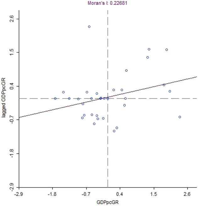
Figures 1, 2, 3, 4, 5, 6, 7, 8 were obtained through GeoDa software, data obtained from the OECD databases and shapefiles from Eurostat. The shapefiles were worked with the QGIS software. These figures show the global and local spatial autocorrelation for the GDP per capita growth rates on average over the final quarter of 2017 to the third quarter of 2020 for the OECD countries plus Bulgaria, Costa Rica, Romania and Saudi Arabia. These four OECD non‐member countries were considered because of the availability of statistical information in the database for these nations and the importance of these states for international geostrategy, in the European Union and in the Middle East. In these figures, global spatial autocorrelation is assessed directly through Moran’s I statistics that is expected to assume values between 0 and −1 (for negative spatial correlation in each variable) and 0 and 1 (for positive spatial correlation). The local spatial autocorrelation is analysed with LISA cluster maps. In the high–high and low–low clusters, there are positive spatial autocorrelations for high and low values, respectively. The low–high and high–low clusters are associated with negative spatial autocorrelation (Anselin et al., 2006; GeoDa, 2021).

FIGURE 1.

Global spatial autocorrelation for the average gross domestic product per capita growth rate, from the final quarter of 2017 to the final quarter of 2019, for OECD countries plus the four non‐member states

FIGURE 2.

Local spatial autocorrelation for the average gross domestic product per capita growth rate, from the final quarter of 2017 to the final quarter of 2019, for OECD countries plus the four non‐member states

FIGURE 3.

Global spatial autocorrelation for the average gross domestic product per capita growth rate, from the final quarter of 2017 to the final quarter of 2019, for OECD countries

FIGURE 4.

Local spatial autocorrelation for the average gross domestic product per capita growth rate, from the final quarter of 2017 to the final quarter of 2019, for OECD countries

FIGURE 5.

Global spatial autocorrelation for the average gross domestic product per capita growth rate, from the final quarter of 2017 to the third quarter of 2020, for OECD countries plus the four non‐member states

FIGURE 6.

Local spatial autocorrelation for the average gross domestic product per capita growth rate, from the final quarter of 2017 to the third quarter of 2020, for OECD countries plus the four non‐member states

FIGURE 7.

Global spatial autocorrelation for the average gross domestic product per capita growth rate, from the final quarter of 2017 to the third quarter of 2020, for OECD countries

FIGURE 8.

Local spatial autocorrelation for the average gross domestic product per capita growth rate, from the final quarter of 2017 to the third quarter of 2020, for OECD countries

Figure 1 demonstrates that, before the pandemic’s impact, for the OECD countries plus Bulgaria, Costa Rica, Romania and Saudi Arabia, there is positive global spatial autocorrelation for the average GDP per capita growth rates; however, this is not so strong when considering the value for the Moran's I statistics (0.312). Figure 2 confirms the weak spatial autocorrelation across the countries considered and shows that there is positive local spatial autocorrelation for higher values in Romania, Lithuania and Latvia and negative spatial autocorrelation for the United States (high–low) and the United Kingdom (low–high). This framework highlights promising perspectives regarding the convergence process of the GDP per capita of the OECD countries and Bulgaria, Costa Rica, Romania and Saudi Arabia.

Considering only the OECD countries (Figures 3 and 4), the results for the spatial autocorrelation are even weaker because of, for example, the absence of the effect from Romania which was verified, in Figure 2, to be a cluster with positive local spatial correlation for higher values of the GDP per capita growth rates. Romania appears here with interesting performances for GDP per capita and is spatially correlated with neighbouring countries in this variable. In terms of policy implementation, this could provide relevant insight for policymakers. These performances for the GDP per capita growth rates and the respective spatial autocorrelation for higher values were also found for Lithuania and Latvia. Considering the lower level of GDP for the Eastern and Central European countries, these interesting performances of the GDP per capita growth rates in Romania, Lithuania and Latvia may support a faster convergence context in the European Union. In fact, the Central and East European countries may bring relevant contributions to the European Union process of convergence (Stanisic et al., 2018). The main objective of the European structural support is to promote faster growth for poorer regions, and it seems that there have been some interesting signs of this, in recent years, from Eastern Europe.

With the Covid‐19 impact during the first three quarters of 2020 (Figures 5, 6, 7, 8), spatial autocorrelation weakened, with the Moran's I statistics assuming results of 0.035 and 0.038, respectively, for global spatial autocorrelation with and without Bulgaria, Costa Rica, Romania and Saudi Arabia. Bulgaria, Costa Rica, Romania and Saudi Arabia are the nations with a more negative GDP per capita growth rate on average, and this contexts had an impact on the results of the spatial autocorrelation. Several countries, in the European Union, were implementing efforts to improve their economic performance and to achieve the targets designated by European institutions. Some of them, such as Portugal and Greece, were recovering from the consequences of other external impacts (financial and economic crises). The Covid‐19 pandemic created new and additional difficulties. These external shocks with their consequent changes of paradigm are, also, sources of opportunities to design and implement innovative approaches in socioeconomic domains (Alsharef et al., 2021). The main question that arises here is how these countries will be able to create advantages from these new challenges.

5. RESULTS OF SIGMA AND BETA CONVERGENCE

The results presented in this section were obtained through the Stata software, considering statistical information from the OECD database for GDP per capita (gross domestic product – expenditure approach; per head, US dollars, volume estimates, fixed PPP, OECD reference year, seasonally adjusted).

5.1. Sigma convergence

Figures 9 and 10 for sigma convergence measured through the coefficient of variation reveal that there are signs of convergence over the final quarter of 2017 to the first quarter of 2019 for the OECD countries, with or without Bulgaria, Costa Rica, Romania and Saudi Arabia. Nonetheless, the dispersion of GDP per capita is greater for those countries that do not belong to the OECD (Figure 9).

FIGURE 9.

Coefficient of variation for GDP per capita, over the period 2017q4–2020q3 and across the OECD countries plus the four non‐member states

FIGURE 10.

Coefficient of variation for GDP per capita, over the period 2017q4–2020q3 and across the OECD countries

The tendencies of divergence verified from the first quarter of 2019 were accentuated with the Covid‐19 pandemic in the beginning of 2020; however, the signs of convergence in the third quarter of 2020 seem to be greater without Bulgaria, Costa Rica, Romania and Saudi Arabia (Figure 10), showing the difficulties of these countries to recuperate economically after external impacts.

Indeed, after a consistent trend of convergence since the beginning of 2018, the second and fourth quarters of 2019 show relevant evidence of divergence among the OECD countries. Some explanations for these signs may be related, for example, to the uncertain trade between China and the United States, Brexit and elections occurring for some large economies.

5.2. Beta convergence

The results presented in Table 2 confirm that the signs of convergence verified over the final quarter of 2017 to the final quarter of 2019 disappeared with the arrival of the Covid‐19 pandemic. In turn, the signs of convergence between 2017 and 2019 were greater without countries which are non‐members of the OECD (−0.239) than with these nations (−0.220). Nonetheless, the Central and East European countries may play a determinant role in the global convergence process, within the European Union framework (Stanisic et al., 2018). The Hausman test shows the preference for fixed effects before the pandemic. In addition, there is evidence that the spatial impacts on the GDP per capita growth rate evolution, over the periods considered, are only statistically significant for the longer period (2017–2020), and these spatial effects come from the dependent variable lagged and from the error term lagged (random spatial effects). These spatial implications for the period 2017–2020 are greater when including Bulgaria, Costa Rica, Romania and Saudi Arabia. The coefficients of the spatial effects have a positive influence on the GDP per capita growth rate, showing a direct relationship between these variables. Considering that, from the previous section for the spatial autocorrelation assessment, spatial autocorrelation became weaker after the first quarter of 2020 (when the GDP per capita growth rates showed poorer performance) and that these frameworks were slightly worse with the non‐OECD members, the pandemic reduced the spread effects over neighbouring countries. On the other hand, these contexts had a direct impact on economic growth performance, more so when Bulgaria, Costa Rica, Romania and Saudi Arabia were considered.

TABLE 2.

Results from the conditional convergence model, for GDP per capita, with panel data and spatial effects over the period 2017q4–2020q3 and across OECD countries plus the four non‐member states

Countries/period	OECD + Bulgaria, Costa Rica, Romania and Saudi Arabia/2017q4–2019q4		OECD/2017q4–2019q4		OECD + Bulgaria, Costa Rica, Romania and Saudi Arabia/2017q4–2020q3		OECD/2017q4–2020q3
Model	Fixed effects	Random effects	Fixed effects	Random effects	Fixed effects	Random effects	Fixed effects	Random effects
Constant		0.025 (1.380) [0.169]		0.013 (0.680) [0.496]		−0.046 (−1.240) [0.216]		−0.066 (−1.520) [0.129]
Logarithm of GDP per capita of the previous year	−0.220* (−5.210) [0.000]	−0.002 (−1.170) [0.241]	−0.239* (−5.490) [0.000]	−0.000 (−0.490) [0.621]	0.007 (0.080) [0.936]	0.003 (1.040) [0.300]	−0.045 (−0.440) [0.662]	0.005 (1.340) [0.179]
Lagged independent variable (logarithm of GDP per capita of the previous year)	0.148 (1.740)** [0.082]	−0.000 (−0.140) [0.892]	0.125 (1.460) [0.145]	−0.000 (−0.400) [0.691]	−0.139 (−0.480) [0.629]	0.000 (1.210) [0.228]	0.307 (1.020) [0.309]	0.000 (0.910) [0.364]
Lagged dependent variable (GDP per capita growth rate)	−0.074 (−0.360) [0.719]	0.235 (1.360) [0.174]	−0.089 (−0.420) [0.674]	0.185 (1.030) [0.303]	0.627* (5.370) [0.000]	0.663* (6.650) [0.000]	0.580* (4.230) [0.000]	0.647* (5.850) [0.000]
Lagged error term	0.010 (0.050) [0.960]	−0.181 (−0.880) [0.380]	−0.066 (−0.310) [0.753]	−0.165 (−0.780) [0.437]	0.635* (5.530) [0.000]	0.581* (4.920) [0.000]	0.574* (4.100) [0.000]	0.485* (3.370) [0.001]
Hausman test	34.680* [0.000]		36.960* [0.000]		0.000 [0.966]		0.080 [0.999]

Note:

^*, statistically significant at 5%;

^**, statistically significant at 10%.

6. CONCLUSIONS

The socioeconomic dynamics created over recent years, between the quarters of 2017 and 2019, showed interesting evidence of convergence among the OECD countries, where some Central and Eastern European Countries (including the non‐member Romania) may play a relevant role in European Union development. Nonetheless, the Covid‐19 pandemic changed some paradigms and brought about new challenges for more vulnerable economies, compromising the efforts made around the world to promote balanced development.

The literature review highlights the relevance of GDP per capita for economic performance assessments, namely when it is intended to analyse processes of convergence. On the other hand, the scientific literature shows that the economic growth of nations is vulnerable to external impacts, such as the financial crisis and the Covid‐19 pandemic. This vulnerability is particularly visible in weaker economies, where the problems of development and the capacity of response to unexpected challenges are more accentuated. Considering that the processes of convergence are contexts where poorer countries attempt to catch up to the levels of growth of wealthier ones, the contexts created by these external forces are especially relevant in designing strategies which support the mitigation of trends in socioeconomic divergence. In any case, it remains unclear how global countries will be able to deal with the damage sustained from the pandemic and how they will be able to project innovative approaches to future challenges.

The data analysis reveals that the United States, Korea and some countries from the European Union (Ireland, Romania, Hungary, Lithuania, Poland, Bulgaria, Latvia, Estonia, Slovak Republic, Portugal, Slovenia, Denmark and the Czech Republic) were the leading countries, in terms of GDP per capita growth rates on average, before the pandemic. The economic impacts from Covid‐19 were greater in countries with a higher incidence rate from the pandemic, in terms of total cases – with the exception of Greece, which appears among some of the countries with worse GDP per capita growth rates, but with a comparatively low number of cases. This shows the vulnerability of more fragile economies to unexpected events. Indeed, there are groups of countries in the European Union which have implemented great effort, over a number of years, to achieve the goals proposed by international and European institutions who now see their situations being brought back to the start or, in some cases, worse. These new contexts are real opportunities to redesign and think about newer, more sustainable and adjusted paradigms for climate change and global warming. It seems that these current times may be one of the last chances to change the thinking behind economic development and its impact on other societal domains.

The spatial assessment highlights that there are signs of spatial autocorrelation which were stronger for the period before the pandemic, and in this case, the spatial correlations were even greater when also considering the non‐members of the OECD – for example, Romania, which has positive local spatial autocorrelations for higher values. After Covid‐19, the contexts are different and the spatial correlations are higher when the non‐members are not considered, showing that there is a diverse pattern of these countries in the reaction to the pandemic; however, the differences are not so relevant.

The results for sigma and beta convergence confirm the findings highlighted before. In fact, the dispersion of GDP per capita (measured through the coefficient of variation) is greater when considering the non‐members of the OECD, and the signs of convergence on the third quarter of 2020 are weaker. In addition, the results from the regressions for the beta convergence reveal that the evidence of convergence disappeared with the pandemic.

As a few final remarks, it is worth noting that the Covid‐19 pandemic had strong implications for OECD economic growth and the convergence processes between these countries. In terms of practical implications, the findings obtained within this study may provide interesting support for public institutions, international organizations, governments and policymakers. After the pandemic, it will be important that the European Union institutions consider Eastern and Central countries, such as Romania, Lithuania and Latvia, when implementing strategies for GDP per capita growth that may be spread to neighbouring countries and promote convergence processes. In any case, during the pandemic and in the future, it could be important to design specific policy instruments for the economies which were more susceptible to the impacts of Covid‐19, such as the four non‐members OECD countries considered in this research. In fact, these countries are determinants for international geostrategy and the creation of measures by the European Union institutions and international organizations. It will be crucial to promote a balanced development in the coming years, to prevent global and localized social and political instability.

For future research, it might be interesting to analyse the effects of the pandemic on the economic growth dynamic over a larger period. It could also bring relevant inputs for assessing the impact of other variables, related to the new paradigm associated with the pandemic, in the GDP per capita process of convergence in OECD countries. For example, it could be important to analyse how changes in the organization of the workforce may affect the global process of economic convergence. Online working has come to stay, and this has had several direct and indirect implications on socioeconomic contexts which could be assessed further.

Martinho, V. J. P. D. (2021). Impact of Covid‐19 on the convergence of GDP per capita in OECD countries. Regional Science Policy & Practice, 13(S1), 55–72. 10.1111/rsp3.12435

REFERENCES

- Abel, G. J. , & Gietel‐Basten, S. (2020). International remittance flows and the economic and social consequences of COVID‐19. Environment and Planning a‐Economy and Space, 52, 1480–1482. 10.1177/0308518X20931111 [DOI] [Google Scholar]
- Adamu, P. , Kaliappan, S. R. , Sirag, A. , & Chenbap, R. J. (2017). Can well‐being between sub‐Saharan Africa (SSA) and Organization for Economic Cooperation and Development (OECD) member countries converge? GeoJournal, 82, 369–377. 10.1007/s10708-015-9687-6 [DOI] [Google Scholar]
- Akeel, H. , & Khoj, H. (2020). Is education or Real GDP per capita helped countries staying at home during Covid‐19 pandemic: Cross‐section evidence? Entrepreneurship and Sustainability Issues, 8, 841–852. 10.9770/jesi.2020.8.1(56) [DOI] [Google Scholar]
- Alexa, D. , Cismas, L. M. , Rus, A. V. , & Silaghi, M. I. P. (2019). Economic growth, competitiveness and convergence in the European regions. A spatial model estimation. Economic Computation and Economic Cybernetics Studies and Research, 53, 107–124. 10.24818/18423264/53.1.19.07 [DOI] [Google Scholar]
- Alsharef, A. , Banerjee, S. , Uddin, S. M. J. , Albert, A. , & Jaselskis, E. (2021). Early impacts of the COVID‐19 pandemic on the United States construction industry. International Journal of Environmental Research and Public Health, 18, 1559. 10.3390/ijerph18041559 [DOI] [PMC free article] [PubMed] [Google Scholar]
- Altinay, G. (2003). Estimating growth rate in the presence of serially correlated errors. Applied Economics Letters, 10, 967–970. 10.1080/1350485032000165485 [DOI] [Google Scholar]
- Angeriz, A. , Mccombie, J. , & Roberts, M. (2008). New estimates of returns to scale and spatial spillovers for EU regional manufacturing, 1986‐2002. International Regional Science Review, 31, 62–87. 10.1177/0160017607306750 [DOI] [Google Scholar]
- Anselin, L. , Syabri, I. , & Kho, Y. (2006). GeoDa: An introduction to spatial data analysis. Geographical Analysis, 38, 5–22. 10.1111/j.0016-7363.2005.00671.x [DOI] [Google Scholar]
- Asfahan, S. , Shahul, A. , Chawla, G. , Dutt, N. , Niwas, R. , & Gupta, N. (2020). Early trends of socio‐economic and health indicators influencing case fatality rate of COVID‐19 pandemic. Monaldi Archives for Chest Disease, 90, 451–457. 10.4081/monaldi.2020.1388 [DOI] [PubMed] [Google Scholar]
- Ayouba, K. , Le Gallo, J. , & Vallone, A. (2020). Beyond GDP: An analysis of the socio‐economic diversity of European regions. Applied Economics, 52, 1010–1029. 10.1080/00036846.2019.1646885 [DOI] [Google Scholar]
- Azhgaliyeva, D. , Yang, L. , & Liddle, B. (2020). An empirical analysis of energy intensity and the role of policy instruments. Energy Policy, 145, 111773. 10.1016/j.enpol.2020.111773 [DOI] [Google Scholar]
- Balash, V. , Balash, O. , Faizliev, A. , & Chistopolskaya, E. (2020). Economic growth patterns: Spatial econometric analysis for Russian regions. Information, 11, 289. 10.3390/info11060289 [DOI] [Google Scholar]
- Barro, R. J. (1991). Economic growth in a cross section of countries. The Quarterly Journal of Economics, 106, 407–443. 10.2307/2937943 [DOI] [Google Scholar]
- Barro, R. J. , Sala‐I‐Martin, X. , Blanchard, O. J. , & Hall, R. E. (1991). Convergence across states and regions. Brookings Papers on Economic Activity, 107–182. 10.2307/2534639 [DOI] [Google Scholar]
- Batog, B. , & Batog, J. (2015). Conditional income convergence in the European Union: R&d spending and export influence. Transformations in Business and Economics, 14, 407–418. [Google Scholar]
- Bentzen, J. (2005). Testing for catching‐up periods in time‐series convergence. Economics Letters, 88, 323–328. 10.1016/j.econlet.2005.04.001 [DOI] [Google Scholar]
- Bentzen, J. (2015). Comparing data sources of real GDP in purchasing power parities. Applied Economics Letters, 22, 1303–1308. 10.1080/13504851.2015.1026576 [DOI] [Google Scholar]
- Bhattacharjee, A. , & Jensen‐Butler, C. (2013). Estimation of the spatial weights matrix under structural constraints. Regional Science and Urban Economics, 43, 617–634. 10.1016/j.regsciurbeco.2013.03.005 [DOI] [Google Scholar]
- Bishop, P. (2013). The spatial distribution of personal insolvencies in England and Wales, 2000‐2007. Regional Studies, 47, 419–432. 10.1080/00343404.2011.581653 [DOI] [Google Scholar]
- Campo, K. N. , Rodrigues, I. C. P. , Lopes, E. S. N. , & Gabriel, L. P. (2020). Early public research funding response to COVID‐19 pandemic in Brazil. Revista da Sociedade Brasileira de Medicina Tropical, 53, e20200522. 10.1590/0037-8682-0522-2020 [DOI] [PMC free article] [PubMed] [Google Scholar]
- Celbis, M. G. , Wong, P.‐H. , & Guznajeva, T. (2018). Regional integration and the economic geography of Belarus. Eurasian Geography and Economics, 59, 462–495. 10.1080/15387216.2019.1573694 [DOI] [Google Scholar]
- Chatterji, M. (1992). Convergence clubs and endogenous growth. Oxford Review of Economic Policy, 8, 57–69. [Google Scholar]
- Cracolici, M. F. , Cuffaro, M. , & Nijkamp, P. (2007). Geographical distribution of unemployment: An analysis of provincial differences in Italy. Growth and Change, 38, 649–670. 10.1111/j.1468-2257.2007.00391.x [DOI] [Google Scholar]
- Cunado, J. , Gil‐Alana, L. A. , & De Gracia, F. P. (2003). Empirical evidence on real convergence in some OECD countries. Applied Economics Letters, 10, 173–176. 10.1080/1350485022000044066 [DOI] [Google Scholar]
- Cunado, J. , Gil‐Alana, L. A. , & de Gracia, F. P. (2006). Additional empirical evidence on real convergence: A fractionally integrated approach. Review of World Economics, 142, 67–91. 10.1007/s10290-006-0057-9 [DOI] [Google Scholar]
- Daban, T. , Domenech, R. , & Molinas, C. (1997). International and intertemporal comparisons of real product in OECD countries: A growth sensitivity analysis. Review of Income and Wealth, 43, 33–48. 10.1111/j.1475-4991.1997.tb00199.x [DOI] [Google Scholar]
- Dall'Erba, S. , Percoco, M. , & Piras, G. (2008). The European regional growth process revisited. Spatial Economic Analysis, 3, 7–25. 10.1080/17421770701733399 [DOI] [Google Scholar]
- de la Paz, P. T. , Lopez, E. , & Juarez, F. (2017). Ripple effect on housing prices. Evidence from tourist Markets in Alicante, Spain. International Journal of Strategic Property Management, 21, 1–14. 10.3846/1648715X.2016.1241192 [DOI] [Google Scholar]
- Diebolt, C. , Mishra, T. , Ouattara, B. , & Parhi, M. (2013). Democracy and economic growth in an interdependent world. Review of International Economics, 21, 733–749. 10.1111/roie.12067 [DOI] [Google Scholar]
- Duan, H. K. , Hu, H. , Vasarhelyi, M. , Rosa, F. S. , & Lyrio, M. V. L. (2020). Open government data (OGD) driven decision aid: A predictive model to monitor COVID‐19 and support decisions in a Brazilian state. Revista Do Servico Publico, 71, 140–164. 10.21874/rsp.v71i0.5009 [DOI] [Google Scholar]
- Eurostat . (2021). Several Statistics and Information.
- Ezcurra, R. , Iraizoz, B. , & Rapun, M. (2008). Regional efficiency in the European Union. European Planning Studies, 16, 1121–1143. 10.1080/09654310802315807 [DOI] [Google Scholar]
- Fay, M. , De Rosa, D. , & Pauna, C. (2008). Product market regulation in Romania: A comparison with OECD countries – part I. Romanian Journal of Economic Forecasting, 9, 5–34. [Google Scholar]
- Felice, E. (2019). The roots of a dual equilibrium: GDP, productivity, and structural change in the Italian regions in the long run (1871‐2011). European Review of Economic History, 23, 499–528. 10.1093/ereh/hey018 [DOI] [Google Scholar]
- Figari, F. , Fiorio, C. , Gandullia, L. , & Montorsi, C. (2020). The resilience of the Italian social protection system at the beginning of Covid‐19 outbreak: Territorial evidence. Politica Economica, 36, 3–34. 10.1429/97786 [DOI] [Google Scholar]
- Fujita, M. , Krugman, P. , & Venables, A. J. (2001). The spatial economy: Cities, regions, and international trade. The MIT Press. [Google Scholar]
- Furkova, A. (2020). Does spatial heterogeneity matter in the EU Regions’ convergence income process? Ekonomicky Casopis, 68, 677–698. 10.31577/ekoncas.2020.07.02 [DOI] [Google Scholar]
- Gao, X. , Li, T. , & Cao, X. (2019). Spatial fairness and changes in transport infrastructure in the Qinghai‐Tibet plateau area from 1976 to 2016. Sustainability, 11, 589. 10.3390/su11030589 [DOI] [Google Scholar]
- GeoDa . (2021). GeoDa Software.
- German‐Soto, V. , & Brock, G. (2015). Strength in diversity: A spatial dynamic panel analysis of Mexican regional industrial convergence, 1960‐2003. Comparative Economic Studies, 57, 183–202. 10.1057/ces.2014.42 [DOI] [Google Scholar]
- German‐Soto, V. , & Escobedo Sagaz, J. L. (2011). Has trade liberalization increased economic inequality among the Mexican states? An analysis from a spatial econometric perspective. Economia Mexicana‐Nueva Epoca, 20, 37–77. [Google Scholar]
- Gomez‐Zaldivar, M. , Fonseca, F. J. , Mosqueda, M. T. , & Gomez‐Zaldivar, F. (2020). Spillover effects of economic complexity on the per capita GDP growth rates of Mexican states, 1993‐2013. Estudios de Economia, 47, 221–243. 10.4067/S0718-52862020000200221 [DOI] [Google Scholar]
- Good, D. F. , & Ma, T. (1999). The economic growth of Central and Eastern Europe in comparative perspective, 1870‐1989. European Review of Economic History, 3, 103–137. 10.1017/S1361491699000076 [DOI] [Google Scholar]
- Goschin, Z. (2017). Exploring regional economic convergence in Romania. A spatial modeling approach. Eastern Journal of European Studies, 8, 127–146. [Google Scholar]
- Gostomski, E. , & Michalowski, T. (2015). Negotiations on the transatlantic free trade area. Effects of the proposed agreement on the economies of the European Union and the United States of America. European Integration Studies, 0, 127–138. 10.5755/j01.eis.0.9.12801 [DOI] [Google Scholar]
- Greiner, A. , & Owusu, B. K. (2020). How to spend 750 billion euro? Applying sacrifice theory to determine Covid‐19 compensations in the EU. Economics Bulletin, 40, 2457–2470. 10.2139/ssrn.3634483 [DOI] [Google Scholar]
- He, S. , Fang, C. , & Zhang, W. (2017). A geospatial analysis of multi‐scalar regional inequality in China and in metropolitan regions. Applied Geography, 88, 199–212. 10.1016/j.apgeog.2017.08.017 [DOI] [Google Scholar]
- Henley, A. (2005). On regional growth convergence in Great Britain. Regional Studies, 39, 1245–1260. 10.1080/00343400500390123 [DOI] [Google Scholar]
- Huynh, T. L. D. (2020). Does culture matter social distancing under the COVID‐19 pandemic? Safety Science, 130, 104872. 10.1016/j.ssci.2020.104872 [DOI] [PMC free article] [PubMed] [Google Scholar]
- Islam, N. (1995). Growth empirics: A panel data approach. The Quarterly Journal of Economics, 110, 1127–1170. 10.2307/2946651 [DOI] [Google Scholar]
- Ju, H. , & Zhang, X. (2020). Spatial econometrics analysis on the convergence of low‐carbon economic growth efficiency in the Yangtze River Economic Belt. Environmental Engineering and Management Journal, 19, 1115–1123. [Google Scholar]
- Kaldor, N. (1966). Causes of the slow rate of economic growth of the United Kingdom: An inaugural lecture. Cambridge University Press. [Google Scholar]
- Kaldor, N. (1984). Causes of growth and stagnation in the world economy. Cambridge University Press. [Google Scholar]
- Kousi, T. , Mitsi, L.‐C. , & Simos, J. (2021). The early stage of COVID‐19 outbreak in Greece: A review of the national response and the socioeconomic impact. International Journal of Environmental Research and Public Health, 18, 322. 10.3390/ijerph18010322 [DOI] [PMC free article] [PubMed] [Google Scholar]
- Labidi, M. A. (2019). Development policy and regional economic convergence: The case of Tunisia. Regional Science Policy and Practice, 11, 583–595. 10.1111/rsp3.12206 [DOI] [Google Scholar]
- Le Gallo, J. (2004). Space‐time analysis of GDP disparities among European regions: A Markov chains approach. International Regional Science Review, 27, 138–163. 10.1177/0160017603262402 [DOI] [Google Scholar]
- Lee, C.‐C. , & Chang, C.‐P. (2009). Stochastic convergence of per capita carbon dioxide emissions and multiple structural breaks in OECD countries. Economic Modelling, 26, 1375–1381. 10.1016/j.econmod.2009.07.003 [DOI] [Google Scholar]
- Li, G. , & Fang, C. (2014). Analyzing the multi‐mechanism of regional inequality in China. Annals of Regional Science, 52, 155–182. 10.1007/s00168-013-0580-2 [DOI] [Google Scholar]
- Li, H. , & Haynes, K. E. (2011). Economic structure and regional disparity in China: Beyond the Kuznets transition. International Regional Science Review, 34, 157–190. 10.1177/0160017610386480 [DOI] [Google Scholar]
- Li, M. , Li, C. , & Zhang, M. (2018). Exploring the spatial spillover effects of industrialization and urbanization factors on pollutants emissions in China’s Huang‐Huai‐Hai region. Journal of Cleaner Production, 195, 154–162. 10.1016/j.jclepro.2018.05.186 [DOI] [Google Scholar]
- Liontakis, A. , & Kremmydas, D. (2014). Food inflation in the European Union: Distribution analysis and spatial effects. Geographical Analysis, 46, 148–164. 10.1111/gean.12033 [DOI] [Google Scholar]
- Liu, Q. , Wang, S. , Li, B. , & Zhang, W. (2020). Dynamics, differences, influencing factors of eco‐efficiency in China: A spatiotemporal perspective analysis. Journal of Environmental Management, 264, 110442. 10.1016/j.jenvman.2020.110442 [DOI] [PubMed] [Google Scholar]
- Liu, R. , Li, T. , & Greene, R. (2020). Migration and inequality in rental housing: Affordability stress in the Chinese cities. Applied Geography, 115, 102138. 10.1016/j.apgeog.2019.102138 [DOI] [Google Scholar]
- Ma, F. , Wang, W. , Sun, Q. , Liu, F. , & Li, X. (2018). Integrated transport efficiency and its spatial convergence in China's provinces: A super‐SBM DEA model considering undesirable outputs. Applied Sciences‐Basel, 8, 1698. 10.3390/app8091698 [DOI] [Google Scholar]
- Martinho, V. D. , Sanchez‐Carreira, M. D. C. , & Reis Mourão, P. (2020). Transnational economic clusters: The case of the Iberian Peninsula. Regional Science Policy and Practice, 1–18. 10.1111/rsp3.12346 [DOI] [Google Scholar]
- Martinho, V. J. P. D. (2019a). Social justice: Disparities in average earnings across Portuguese municipalities. Social Sciences, 8, 125. 10.3390/socsci8040125 [DOI] [Google Scholar]
- Martinho, V. J. P. D. (2019b). Testing for structural changes in the European Union's agricultural sector. Agriculture, 9, 92. 10.3390/agriculture9050092 [DOI] [Google Scholar]
- Martinho, V. J. P. D. , & Barandela, J. S. (2020). Exploring dynamics between the socioeconomic sectors from north of Portugal and Galicia. Regional Science Inquiry, 12, 221–228. [Google Scholar]
- Megyesiova, S. , & Lieskovska, V. (2018). Analysis of the sustainable development indicators in the OECD countries. Sustainability, 10, 4554. 10.3390/su10124554 [DOI] [Google Scholar]
- Nan, Y. , Li, Q. , Cai, H. , & Zhou, Q. (2020). Are there industrial SO2 convergences in China’s prefecture‐level cities? New evidence from a spatial econometric perspective. Energy & Environment, 31, 440–460. 10.1177/0958305X19869390 [DOI] [Google Scholar]
- OECD . (2021). Several Statistics.
- Olejnik, A. (2008). Using the spatial autoregressively distributed lag model in assessing the regional convergence of per‐capita income in the EU25. Papers in Regional Science, 87, 371–384. 10.1111/j.1435-5957.2008.00190.x [DOI] [Google Scholar]
- Paez, A. , Lopez, F. A. , Menezes, T. , Cavalcanti, R. , & da Pitta, M. G. d. R. (2021). A Spatio‐temporal analysis of the environmental correlates of COVID‐19 incidence in Spain. Geographical Analysis. 10.1111/gean.12241 [DOI] [PMC free article] [PubMed] [Google Scholar]
- Patacchini, E. , & Rice, P. (2007). Geography and economic performance: Exploratory spatial data analysis for Great Britain. Regional Studies, 41, 489–508. 10.1080/00343400600928384 [DOI] [Google Scholar]
- QGIS.org . (2021). QGIS Geographic Information System. QGIS Association. [Google Scholar]
- Rey, S. J. , & Montouri, B. D. (1999). US regional income convergence: A spatial econometric perspective. Regional Studies, 33, 143–156. 10.1080/00343409950122945 [DOI] [Google Scholar]
- Rey, S. J. (2018). Bells in space: The spatial dynamics of US interpersonal and interregional income inequality. International Regional Science Review, 41, 152–182. 10.1177/0160017615614899 [DOI] [Google Scholar]
- Rodriguez‐Pose, A. (1999). Convergence or divergence? Types of regional responses to socio‐economic change in Western Europe. Tijdschrift voor Economische en Sociale Geografie, 90, 363–378. 10.1111/1467-9663.00079 [DOI] [Google Scholar]
- Royuela, V. , & Adolfo Garcia, G. (2015). Economic and social convergence in Colombia. Regional Studies, 49, 219–239. 10.1080/00343404.2012.762086 [DOI] [Google Scholar]
- Sala‐i‐Martin, X. X. (1996). Regional cohesion: Evidence and theories of regional growth and convergence. European Economic Review, 40, 1325–1352. 10.1016/0014-2921(95)00029-1 [DOI] [Google Scholar]
- Salvati, L. , Benassi, F. , Miccoli, S. , Rabiei‐Dastjerdi, H. , & Matthews, S. A. (2020). Spatial variability of total fertility rate and crude birth rate in a low‐fertility country: Patterns and trends in regional and local scale heterogeneity across Italy, 2002–2018. Applied Geography, 124, 102321. 10.1016/j.apgeog.2020.102321 [DOI] [Google Scholar]
- Santos, E. , Oliveira, M. , Ratten, V. , Tavares, F. O. , & Tavares, V. C. (2020). A reflection on explanatory factors for COVID‐19: A comparative study between countries. Thunderbird International Business Review, 63, 285–301. 10.1002/tie.22188 [DOI] [Google Scholar]
- Santos‐Marquez, F. , & Mendez, C. (2020). Regional convergence, spatial scale, and spatial dependence: Evidence from homicides and personal injuries in Colombia 2010‐2018. Regional Science Policy and Practice, 1–23. 10.1111/rsp3.12356 [DOI] [Google Scholar]
- Sardadvar, S. , & Rocha‐Akis, S. (2016). Interregional migration within the European Union in the aftermath of the Eastern enlargements: A spatial approach. Review of Regional Research‐Jahrbuch Fur Regionalwissenschaft, 36, 51–79. 10.1007/s10037-015-0100-1 [DOI] [Google Scholar]
- Sarker, M. R. (2021). Labor market and unpaid works implications of COVID‐19 for Bangladeshi women. Gender, Work and Organization. 10.1111/gwao.12587 [DOI] [PMC free article] [PubMed] [Google Scholar]
- Shrestha, S. S. , Thompson, T. J. , Kirtland, K. A. , Gregg, E. W. , Beckles, G. L. , Luman, E. T. , Barker, L. E. , & Geiss, L. S. (2016). Changes in disparity in county‐level diagnosed diabetes prevalence and incidence in the United States, between 2004 and 2012. PLoS ONE, 11, e0159876. 10.1371/journal.pone.0159876 [DOI] [PMC free article] [PubMed] [Google Scholar]
- Silveira‐Neto, R. , & Azzoni, C. R. (2006). Location and regional income disparity dynamics: The Brazilian case. Papers in Regional Science, 85, 599–613. 10.1111/j.1435-5957.2006.00099.x [DOI] [Google Scholar]
- Smetkowski, M. (2015). Spatial patterns of regional economic development in central and eastern European countries. Geographia Polonica, 88, 539–555. 10.7163/GPol.0033 [DOI] [Google Scholar]
- Solow, R. M. (1956). A contribution to the theory of economic growth. The Quarterly Journal of Economics, 70, 65–94. 10.2307/1884513 [DOI] [Google Scholar]
- Stanisic, N. , Makojevic, N. , & Curcic, T. T. (2018). The EU enlargement and income convergence: Central and Eastern European countries vs. Western Balkan countries. Entrepreneurial Business and Economics Review, 6, 29–41. 10.15678/EBER.2018.060302 [DOI] [Google Scholar]
- Stata . (2021). Stata: Software for Statistics and Data Science.
- StataCorp . (2017a). Stata 15 base reference manual. Stata Press. [Google Scholar]
- StataCorp . (2017b). Stata statistical software: Release 15. StataCorp LLC. [Google Scholar]
- Su, H. (2020). Performance audit of carbon emission intensity in Chinese inland and coastal areas. Journal of Coastal Research, 115, 451–455. 10.2112/JCR-SI115-126.1 [DOI] [Google Scholar]
- Taylor, A. M. , & Williamson, J. G. (1997). Convergence in the age of mass migration. European Review of Economic History, 1, 27–63. 10.1017/S1361491697000038 [DOI] [Google Scholar]
- Tselios, V. (2008). Income and educational inequalities in the regions of the European Union: Geographical spillovers under welfare state restrictions. Papers in Regional Science, 87, 403–430. 10.1111/j.1435-5957.2008.00191.x 403‐U123 [DOI] [Google Scholar]
- Verdoorn, P. J. (1949). Fattori che regolano lo sviluppo della produttività del lavoro. Ed. L'industria. [Google Scholar]
- Worldometer . (2021). Coronavirus Statistics.
- Zhang, W. , Pan, X. , Yan, Y. , & Pan, X. (2017). Convergence analysis of regional energy efficiency in China based on large‐dimensional panel data model. Journal of Cleaner Production, 142, 801–808. 10.1016/j.jclepro.2016.09.096 [DOI] [Google Scholar]
- Ziesemer, T. H. W. (2010). The impact of the credit crisis on poor developing countries: Growth, worker remittances, accumulation and migration. Economic Modelling, 27, 1230–1245. 10.1016/j.econmod.2010.02.008 [DOI] [Google Scholar]