Polygonal surface processing and mesh generation tools for the numerical simulation of the cardiac function

Abstract

In order to simulate the cardiac function for a patient‐specific geometry, the generation of the computational mesh is crucially important. In practice, the input is typically a set of unprocessed polygonal surfaces coming either from a template geometry or from medical images. These surfaces need ad‐hoc processing to be suitable for a volumetric mesh generation. In this work we propose a set of new algorithms and tools aiming to facilitate the mesh generation process. In particular, we focus on different aspects of a cardiac mesh generation pipeline: (1) specific polygonal surface processing for cardiac geometries, like connection of different heart chambers or segmentation outputs; (2) generation of accurate boundary tags; (3) definition of mesh‐size functions dependent on relevant geometric quantities; (4) processing and connecting together several volumetric meshes. The new algorithms—implemented in the open‐source software vmtk—can be combined with each other allowing the creation of personalized pipelines, that can be optimized for each cardiac geometry or for each aspect of the cardiac function to be modeled. Thanks to these features, the proposed tools can significantly speed‐up the mesh generation process for a large range of cardiac applications, from single‐chamber single‐physics simulations to multi‐chambers multi‐physics simulations. We detail all the proposed algorithms motivating them in the cardiac context and we highlight their flexibility by showing different examples of cardiac mesh generation pipelines.

1. We propose a set of algorithms and tools aiming to facilitate and speed‐up the mesh generation process for cardiac geometries.

2. The main novelties regard the polygonal surface processing, the boundary tags definition, the mesh‐size definition, and the volumetric mesh processing.

3. The new algorithms can be combined with each other to create personalized application‐specific pipelines.

4. We demonstrate the robustness and the flexibility of the proposed tools through various examples on different kinds of cardiac geometries.

1. INTRODUCTION

The mathematical and numerical modeling of the cardiac function is a very challenging research topic. ¹ Advances in this field can help to better understand the heart physiology ² , ³ , ⁴ , ⁵ , ⁶ , ⁷ and are promoting a new approach to the study of cardiac pathologies and their treatments. ⁸ , ⁹ , ¹⁰ , ¹¹ , ¹² , ¹³ , ¹⁴

In terms of modeling, the multi‐physics aspects of the cardiac function can be grouped into three main processes: the electrophysiology that takes into account the electric signal propagation and the biochemical processing occurring at cells level; the active and passive mechanics that, driven by the electric signal and by the pressure evolution inside the cardiac chambers, models the movement and the internal stresses of the cardiac muscle; and the fluid‐dynamics that, together with the motion of the four cardiac valves, regulates the blood flow circulation in the entire human body.

From the geometric point of view, the heart is characterized by a very complex anatomy, as illustrated in Figure 1A. Both the ventricular and the atrial muscles are in continuity from the left to the right side of the heart, while they are connected to each other only by the fibrotic tissue of the annuli, which also acts as electrical insulators. ¹⁶ On the contrary, from the hemodynamic point of view, the internal cavities are connected only along the atrioventricular direction, while a clear separation between the right and the left cavities is necessary to divide the oxygenated and the non‐oxygenated blood. ¹⁶ Thus, from the geometric point of view, a complete electro‐mechano‐fluid model of the cardiac function must take into account both the atrio‐ventricular muscle separation and the right–left hemodynamic division. The complexity is furtherly increased by the presence on the endocardium of the papillary muscles and the trabeculae carneae, which make the inner part of the heart a rough and irregular surface, as shown for the ventricles in Figure 1B. Depending on the focus of the study, this geometric complexity can be addressed with a different level of detail, see for example, Figure 1B–D.

FIGURE 1.

On the left (A), an example of heart geometry, elaborated from the Zygote Solid Heart model ¹⁵ : the Left Atrium (LA) and the Left Ventricle (LV) are filled up with oxygenated blood (in red), while the right atrium (RA) and the right ventricle (RV) are full of non‐oxygenated blood (in blue); the ventricular myocardial muscle is shown in transparency, while the atrial muscle—being very thin—is not depicted. On the right (B‐D), the same ventricular geometry depicted with a decreasing level of details; for the most detailed one (B) an inside zoom of the papillary muscles and trabeculae carneae is also shown

Starting from these general considerations, in the literature we can find a variety of computational studies focused on completely different aspects of the cardiac function: standalone electrophysiology simulations ¹⁷ , ¹⁸ , ¹⁹ often focused on particular pathologies and clinical applications ¹³ , ²⁰ ; electromechanics studies ² , ⁷ , ²¹ , ²² ; fluid‐dynamics simulations involving the cardiac valve modeling ²³ , ²⁴ , ²⁵ , ²⁶ , ²⁷ , ²⁸ ; and, more seldom, full electro‐mechano‐fluid simulations of the heart, albeit with some simplifications. ²⁹ , ³⁰

A computational study of the cardiac function, especially in the case of patient‐specific geometries reconstructed from medical images, generally starts from the processing of polygonal surfaces and the generation of a computational mesh. The difficulty of this first pre‐processing step increases with the number of cardiac chambers we aim to address and the level of geometric detail desired. On the one hand, the mesh generation of a smooth left‐ventricle cut at the base (see Figure 1D) can be considered a relatively simple process. On the other hand, dealing with detailed cardiac geometries (see Figure 1B) or with the constraint of creating conforming meshes between the different chambers of the heart can be a very challenging time‐ and manpower‐consuming operation.

Mesh generation is a field characterized by very different techniques. A detailed review of this topic goes beyond the aim of this paper and can be found, for instance, in References 31, 32, 33, 34, 35 Concerning the cardiac field, various application‐specific pipelines have been proposed in literature. ³⁶ , ³⁷ , ³⁸ , ³⁹ , ⁴⁰ , ⁴¹ , ⁴² , ⁴³ , ⁴⁴ , ⁴⁵ , ⁴⁶

In this context, grid‐based techniques ⁴⁷ invariably start from an initial regular grid—for example, the medical image voxel grid—and adapt the mesh till matching the desired geometry—for example, a multi‐label image segmentation. Exploiting such kind of techniques, Prassl et al ³⁸ proposed a pipeline to build detailed biventricular geometries for electrophysiology models. Similarly, Strocchi et al ⁴⁵ generated a cohort of four‐chambers meshes for electro‐mechanical models from high‐resolution CT‐scans, exploiting the integration in the pipeline of an automatic multi‐label segmentation method. ⁴⁸ As a drawback, these methods all rely on a specific kind of image data or segmentation technique. ³⁸ Thus, they are not applicable, for instance, in the case where each chamber is reconstructed from a different image.

Another technique consists in the use of an application‐specific template mesh, that is deformed into each patient‐specific geometry. ³⁹ , ⁴⁰ , ⁴⁶ , ⁴⁹ The template can be an idealized geometry ³⁹ or an atlas built from a large dataset of medical images. ⁵⁰ , ⁵¹ , ⁵² , ⁵³ In this context, Lamata et al, ³⁹ using an idealized biventricular template, proposed a pipeline to generate smooth biventricular hexahedral meshes for mechanics simulations; This et al ⁴⁶ exploit a smooth template geometry of the left‐heart endocardium to perform patient‐specific hemodynamics simulations; Hoogendoorn et al ⁴⁹ adopt an atlas‐based method to perform patient‐specific electrophysiology simulations in smooth biventricular geometries; Zhang et al ⁴⁰ proposed an atlas‐based method to build cubic Hermite finite element meshes of a full‐heart smooth geometry. Recently, template‐based techniques have also been proposed in the context of isogeometric analysis. ⁵⁴ , ⁵⁵ However, all these techniques strongly rely on the features of the template geometry and are strictly related to the application they are designed for. Additionally, they may have difficulty capturing detailed cardiac geometries, due to the significant anatomical variations of the heart. ⁵⁶ , ⁵⁷ , ⁵⁸

In the context of patient‐specific cardiovascular applications, surface‐based techniques such as advancing‐fronts ⁵⁹ , ⁶⁰ , ⁶¹ and Delaunay‐based methods ⁶² still remain very popular. These methods discretize the domain starting from the external polygonal surface and propagate the mesh‐size of the polygonal elements towards the inside of the volume. The main advantage is a full control over the meshing process through, for instance, coarsening or refinement of specific parts of the surface. Moreover, since they can start from the output of any medical image segmentation algorithm, they can accurately reproduce detailed patient‐specific geometries of both healthy or pathological hearts. This is of fundamental importance since, among all the parameters considered for a cardiovascular simulation, recent studies demonstrate how the geometry has a significant impact on the outputs. ⁶³ , ⁶⁴ , ⁶⁵ As a drawback, these methods require triangulated surfaces of sufficient good quality, whereas thin or intersecting surfaces, typical of cardiac segmentation outputs, can be problematic. Consequently, flexible and easy‐to‐use algorithms to process polygonal surfaces are required to make surface‐based techniques more powerful for cardiac mesh generation.

Summarizing, a unique mesh generation pipeline for all the cardiac applications cannot hardly proposed. For this reason, in this paper, in the context of surface‐based techniques, we propose various independent algorithms and tools that can be combined with each other in a flexible way, creating application‐dependent pipelines. In particular, we start from stable algorithms and tools originally designed for vascular surface processing and mesh generation and implemented in the vascular modeling toolkit (vmtk) ^* library ⁶⁶ and we extend them with new specific algorithms developed for cardiac mesh generation. As sketched in Figure 2, the proposed algorithms will address four different tasks: polygonal surface processing; boundary tags definition; mesh‐size definition; volumetric mesh processing. For each of these tasks, we propose new algorithms to facilitate and automatize common steps in a cardiac mesh generation pipeline, overcoming the typical problems related to surface‐based techniques and cardiac mesh generation. The proposed algorithms—publicly available in a fork of vmtk ^† —are released in a unique framework that allows tremendous flexibility in the creation of mesh‐generation pipelines designed for the needs of the specific cardiac model. Thus, the proposed framework can be used to create single‐ or multi‐chamber geometries with different levels of details, depending on the kind of simulation to be performed. This feature can be considered the primary contribution of our paper. Indeed, despite the existence of numerous open‐source or commercial softwares in this area (e.g., Gmsh, ⁶⁷ Netgen, ⁶⁸ Cubit, ⁶⁹ MeshLab, ⁷⁰ Meshmixer, ⁷¹ Meshtool, ⁴⁴ Blender ⁷² ), having all the tools required to build a cardiac computational mesh in a single pipeline can significantly speed‐up this time‐ and manpower‐consuming operation.

FIGURE 2.

A sketch of the cardiac mesh tools covered in this paper, highlighting the four groups into which they are divided

Moreover, the possibility of creating fully‐automatic pipelines for a specific application can also be exploited for clinical studies on huge datasets or to create virtual cohorts of heart models. ⁷³

The outline of the paper is as follows: in Section 2 we illustrate all the proposed algorithms, and for each of them we provide motivations through significant examples in the cardiac context; in Section 3 we combine the proposed algorithms in single pipelines to generate different kinds of cardiac meshes, and show some examples of already published numerical studies focused on different aspects of the cardiac function; a final discussion and the conclusions of our work are drawn in Section 4.

2. METHODS

In Table 1 we summarize all the new algorithms and tools proposed in this paper, underlining their main input and output. As sketched in Figure 2, we can group them into the following four macro‐areas, to each of which we will dedicate a specific section.

1. Polygonal surface processing (Section 2.1). Among the variety of algorithms related to this broad topic, we propose four algorithms designed for specific processing needs in the framework of cardiac applications. In particular, three of them—surface‐connection (Section 2.1.1), boolean‐connection (Section 2.1.2), and harmonic‐connection (Section 2.1.3)—concern different ways to join two separate polygonal surfaces. This operation is of paramount importance in cardiac applications, where the segmentation output can consist of multiple surfaces, for example, the endocardium and the epicardium of the ventricles or different cardiac chambers. Additionally, we also propose an algorithm—surface‐thickening (Section 2.1.4)—to post‐process a cardiac muscular mesh (e.g., an atrium or a ventricle) in order to locally modify its thickness.

2. Boundary tags definition (Section 2.2). While in most engineering applications the geometry can be defined as a CAD model ⁷⁴ and consequently the boundaries are identifiable as part of this model (e.g., by exploiting sharp edges), significant boundaries of cardiovascular geometries (e.g., valvular annuli) could also appear in smooth parts of the domain. In this context, we propose a flexible and precise tool—surface‐tagger (Section 2.2)—to automatically tag a surface by exploiting significant functions defined on it.

3. Array processing and mesh‐size definition (Section 2.3). While for vascular applications the mesh‐size is usually dependent on the local radius of the vessel, ⁶⁶ , ⁷⁵ , ⁷⁶ for complex cardiac geometries (see, for instance, Figure 1B) more than one geometric quantity needs to be considered (e.g., local curvature, muscle thickness). This topic is also linked to the definition of specific arrays on a surface and to their processing. In this context, we propose the surface‐thickness algorithm (Section 2.3.2) to compute the thickness of the cardiac muscle, and the harmonic‐extension algorithm (Section 2.3.1) to extend a field defined only on a part of the surface. Finally, we propose a tool—surface‐mesh‐size (Section 2.3.3)—to combine and manipulate different arrays in order to flexibly define the desired mesh‐size function on a surface.

4. Volumetric mesh processing (Section 2.4). In surface‐based techniques, after the generation of a surface mesh of the desired mesh‐size, the volumetric mesh generation is a straightforward operation based on well‐known algorithms. ⁶⁰ , ⁶² , ⁶⁸ , ⁷⁷ However, for some cardiac applications, additional processing on the volumetric mesh could be necessary. For this purpose, we propose three algorithms: the mesh‐connection algorithm (Section 2.4.1) to connect two disconnected volumetric meshes, for example, two cardiac chambers at their valvular annuli; a local‐refinement algorithm—mesh‐refinement (Section 2.4.2)—based on the constrained Delaunay refinement method of TetGen ⁶² ; and the tet‐hex algorithm (Section 2.4.3) to include in our framework a well‐known strategy to convert tetrahedral meshes into hexahedral ones.

TABLE 1.

List of all the proposed algorithms and tools with their main input and output

Name	Input	Output
surface‐connection (Section 2.1.1)	Two open surfaces separated by a gap	A continuous surface obtained by smoothly connecting two boundaries of the input surfaces
Boolean‐connection (Section 2.1.2)	Two intersecting surfaces	A continuous smooth surface made of regular triangles obtained as the union, the difference, or the intersection of the two inputs
Harmonic‐connection (Section 2.1.3)	An input surface and a reference surface	A continuous surface made of regular triangles obtained by deforming a boundary of the input surface into a boundary of the reference one, and extending the deformation through a harmonic map
Surface‐thickening (Section 2.1.4)	A surface with an array defined on it representing the thickness	A thickened surface in the regions where the input thickness is lower than a threshold
Surface‐tagger (Section 2.2)	A surface with geometric quantities defined on it as arrays	A tagged surface where the boundary tags are created by exploiting different algorithms based on either the manipulation of the input arrays or an interactive graphical interface
Harmonic‐extension (Section 2.3.1)	A surface with a scalar or vector field defined only on a subpart of it	A surface with the input field extended on the whole domain through a harmonic map
Surface‐thickness (Section 2.3.2)	A tagged surface with specific tags for the internal and the external walls	A surface with its thickness defined on it as an array
Surface‐mesh‐size (Section 2.3.3)	A surface with geometric quantities defined on it as arrays	A surface with an additional array representing the mesh‐size, computed by manipulating the input arrays
mesh‐connection (Section 2.4.1)	Two tagged volumetric meshes separated by a gap	A unique volumetric mesh created by generating a connecting volume between two selected regions of the two input meshes
Mesh‐refinement (Section 2.4.2)	A volumetric mesh with a geometric quantity or function defined on it	A volumetric mesh locally refined by exploiting the input array as a sizing function
tet‐hex (Section 2.4.3)	A tetrahedral volumetric mesh	A hexahedral volumetric mesh obtained by subdividing each tetrahedron intro four hexahedra

We conclude this introduction to the proposed algorithms by motivating the choice of vmtk as development environment and summarizing some notations that we will adopt in the following sections. vmtk is a library written in C++ and Python that can be used as a collection of Python scripts linkable to each other in a pipeline, meaning that the output of a script can be automatically used as the input of another script and so on. Moreover many algorithms and tools of vmtk—despite being originally thought for vascular modeling—can also be applied in the cardiac context. We mention in particular the remeshing algorithm, which is able to remesh a surface according to a mesh‐size function defined on it and preserving the geometry of the boundary tags. Moreover, the remeshing can be localized only on a subset of tags, allowing a significant speed‐up when dealing with complex geometries. In the following, the word “remeshing” always refers to the vmtk remeshing algorithm; we refer to Antiga et al ⁶⁶ for more details. Two other fundamental features of vmtk are the embedding of TetGen ⁶² —for the volumetric mesh generation through an efficient version of the Delaunay algorithm ⁶⁰ , ⁷⁷ —and its internal structure based on the VTK library. ⁷⁸ In particular, we use the latter to require user input through a 3D interactive graphical interface.

In the following algorithms, we deal with both 3D domains, 2D manifolds, and 1D curves, depending on the operation to be performed. We assign a specific Greek letter to each of these three cases, by denoting with Ω the 3D volumetric meshes, with ∑ the 2D polygonal surfaces, and with Γ the 1D curves. A closed 1D curve typically appears as a boundary of a polygonal surface. In this context, we often denote it as ring, since the boundary of the cardiovascular surfaces is usually ring‐shaped. If not otherwise specified, we suppose that Ω is made of tetrahedral elements, ∑ of triangles, and Γ of lines. We indicate a surface without boundary as closed surface, the opposite case as open surface. Finally, we denote as unsigned distance the positive scalar function representing the euclidean distance from a reference object and as signed distance the same distance with a positive or negative sign depending on whether the point is outside or inside the reference object, respectively. These distances are computed using the angle weighted pseudonormal algorithm implemented in VTK. ⁷⁹ , ⁸⁰

2.1. Polygonal surface processing

2.1.1. Connection of disconnected surfaces: The surface‐connection algorithm

Motivations

The starting point of a patent‐specific mesh generation pipeline in the cardiovascular context can often be a set of disconnected surfaces separated by a gap. For instance, the generation of a mesh for the simulation of the fluid dynamics in the heart chambers can typically start from the disconnected internal surfaces of the right/left ventricle, the right/left atrium, and the various inlet/outlet vessels. Indeed, all these geometries can be reconstructed independently from different kinds of images and need to be merged in order to create a continuous triangulation. We will see a complete example of a pipeline to generate such kind of fluid‐dynamic mesh in Section 3, whereas here we detail the new algorithm proposed to connect two disconnected surfaces.

Input, output, parameters and options

The algorithm takes as input two non‐overlapping disconnected open surfaces—named ∑₁ and ∑₂. As output, we obtain a unique surface ∑ connecting the two input surfaces from a ring Γ₁ ∈ ∑₁ to a ring Γ₂ ∈ ∑₂ through a smooth continuous triangulation coherent with the shape of the two boundaries. The connecting triangulation is marked with a specific tag. No parameters are required since the algorithm is completely automatic; if ∑₁ or ∑₂ have more than a single boundary ring, a graphical interface allows the user to choose which one to connect.

The surface‐connection algorithm

Our algorithm starts from a random point on Γ₁ and from its closest point on Γ₂, then it iteratively adds a triangle on Γ₁ or on Γ₂ choosing always the triangle with the shortest connecting edge between the two rings. In Figure 3 we show an example where the right atrium ∑₁ and the right ventricle ∑₂ are connected at their boundaries Γ₁ and Γ₂, respectively, located at the tricuspid valve annulus. More in detail the algorithm proceeds as follows:

1. Extract from ∑₁ and ∑₂ all the boundaries, storing them into two sets of N ₁ and N ₂ rings, respectively;

2. select Γ₁ and Γ₂ from the two boundary sets, using a graphical interface if N ₁ > 1 or N ₂ > 1;

3. supposing that Γ₁ and Γ₂ are made of n ₁ and n ₂ points, respectively, select a random point $P_1^0$ on Γ₁ and find the closest point $P_2^0$ on Γ₂. These are the two starting points of the connecting triangulation, that at this stage is made of the set of points $\mathcal{P}=\left\{P_1^0,P_2^0\right\}$ and of an empty set of triangles $\mathcal{T}=\varnothing$;

4. find the two neighbor points of $P_1^0$ and select randomly one of them as $P_1^{*}$;

5. find the two neighbor points of $P_2^0$ and select as $P_2^{*}$ the closest point to $P_1^{*}$;

6. initializing $P_1=P_1^0$, $P_2=P_2^0$, and i = 2 as the counter of the points inserted in $\mathcal{P}$, proceed as follows while i ≤ (n ₁ + n ₂):

   1. compute the distances $d_1=\mid P_1^{*}-P_2\mid$ and $d_2=\mid P_2^{*}-P_1\mid$;

   2. if d ₁ < d ₂, then set $P^{*}=P_1^{*}$ (red‐triangle case of Figure 3), else set $P^{*}=P_2^{*}$ (green‐triangle case of Figure 3);

   3. insert P ^* into the set of points $\mathcal{P}=\mathcal{P}\cup \left\{P^{*}\right\}$ and increment i = i + 1;

   4. create the triangle T made by the points (P ₁, P ₂, P ^*) and insert it in the triangulation $\mathcal{T}=\mathcal{T}\cup \left\{T\right\}$;

   5. if d ₁ < d ₂, then update P ₁ = P ^* and $P_1^{*}$ as the neighbor of P ₁ not yet inserted in $\mathcal{P}$, otherwise do the same operation for P ₂ and $P_2^{*}$;

7. at the end of the cycle, $\mathcal{P}$ comprises (n ₁ + n ₂ + 1) points. Indeed, only one point between $P_1^0$ and $P_2^0$—that is, the two initial points—has been inserted twice. Thus, at this stage, $\left(P_1=P_1^0\right)⊻\left(P_2=P_2^0\right)$. In order to close the triangulation $\mathcal{T}$, we have to insert the last triangle T ^*—depicted in blue in Figure 3, right—exploiting the point between $P_1^0$ and $P_2^0$ that has not yet been inserted twice: if $P_1=P_1^0$, then T ^* is made of $\left(P_1,P_2,P_2^0\right)$, else T ^* is made of $\left(P_1,P_2,P_1^0\right)$.

8. assign a specific tag to the triangles of the just created connecting triangulation $\mathcal{T}$;

9. merge $\mathcal{T}$ with the two input surfaces by removing duplicate points, creating a unique connected surface $\mathrm{\sum }={\mathrm{\sum }}_1\cup \mathcal{T}\cup {\mathrm{\sum }}_2$.

FIGURE 3.

Connecting the right atrium (∑₁) and the right ventricle (∑₂) at the tricuspid valvular annulus (Γ₁ and Γ₂) using the surface‐connection algorithm. Each generated triangle lies on Γ₁ (red triangles) or Γ₂ (green‐triangles) depending on a minimum distance criterion, while a specific criterion is used for the last triangle that closes the triangulation (in blue)

Discussion

The proposed algorithm demonstrates its robustness when applied to complex cardiac geometries (see Section 3), since it works also when the distance between the rings Γ₁ and Γ₂ varies in a large range. Moreover, we remark that the two rings to be connected can be made of a very different number of points. Indeed, thanks to the minimum distance criterion, the algorithm will insert always the best possible triangle that maintains the smoothness of the connection. Clearly, the resulting triangulation $\mathcal{T}$ can be made of “slim” or “fat” triangles. However, using the capability of vmtk of remeshing only a single tag, the new triangulation can be easily remeshed with an arbitrary mesh‐size, recovering its regularity and, at the same time, maintaining both the shape of the triangulation $\mathcal{T}$ and the conformity with the two input surfaces ∑₁ and ∑₂.

2.1.2. Connection of intersecting surfaces: The boolean‐connection algorithm

Motivations

Outputs of cardiac medical imaging segmentation can be intersecting surfaces. For instance, it is common to reconstruct the endocardium and the epicardium of the left ventricle separately. Since the volume occupied by blood is usually the part with more contrast in a cardiac image—either because of an injection of a contrast agent (like in CT‐scans) or because of specific acquisition protocol (like in cardiac MRI)—the endocardium is reconstructed as the external limit of the blood regions inside the heart. This typically produces a surface that includes a part of the left‐atrial endocardium and of the aortic root. On the contrary, the epicardium is typically reconstructed as a closed surface capped at the valvular annulus. An example of such kind of segmentation outputs is shown in Figure 4, center. In that case the left‐ventricle can be reconstructed by connecting the two surfaces at their intersection. This operation can be achieved with boolean operation between surfaces, ⁸⁰ in particular using the difference boolean operator. However, the output surface can be characterized by irregular triangles and narrowed regions on the intersection zone, as shown in the zoomed box of Figure 4, left. This kind of angular geometry makes the volumetric mesh generation challenging or even not possible without any additional processing. For these reasons, we propose a slightly different approach that generates as output a smoother and already tagged surface ready for volumetric mesh generation, as shown in Figure 4, right, for the aforementioned example.

FIGURE 4.

Comparison between the connection of two intersecting surfaces using classical boolean operations and the proposed boolean‐connection algorithm: on the center, the left‐ventricular epicardium (∑₁) and endocardium (∑₂) as delivered by the segmentation process; on the left, the output of a classical boolean difference operator ∑₁ − ∑₂ which produces irregular triangles and narrowed regions, as depicted in the zoomed box; on the right, the output (∑) of the same difference computed with the boolean‐connection algorithm which generates a smooth surface made of regular triangles and which also assigns the tags of the endocardium (red), the epicardium (gray) and the newly‐generated valvular annulus (blue)

Input, output, parameters and options

Two triangulated surfaces—named ∑₁ and ∑₂—intersecting in one or more closed lines are taken as input. Both ∑₁ and ∑₂ should be closed surfaces, otherwise an undesired output could be produced since the internally‐used signed distance is not robustly defined for open surfaces. Fortunately, polygonal surfaces generated by a medical image segmentation are usually closed. Another requirement is that both surfaces are characterized by outward normals, as it is common for polygonal closed surfaces. Our algorithm provides as output a unique closed surface ∑ defined as the difference, the union, or the intersection between ∑₁ and ∑₂. The two input surfaces are clipped at a user‐defined distance ε from their intersections and then connected using the surface‐connection algorithm. Optionally, the clip operation can be done only on a single input surface. Moreover, the final surface ∑ is remeshed—optionally only near the intersection zone—using a user‐defined constant mesh‐size h.

The boolean‐connection algorithm

1. On ∑₁, compute the signed distance d ₁ from ∑₂ and vice‐versa to obtain d ₂;

2. clip ∑₁ and ∑₂ at their intersection, that is, at the level where d ₁ = d ₂ = 0. Name the two resulting boundary rings Γ₁ and Γ₂. At this stage, ∑₁ and ∑₂ are split into two parts: ${\mathrm{\sum }}_1^{+}$ and ${\mathrm{\sum }}_2^{+}$ where d ₁ ≥ 0 and d ₂ ≥ 0, respectively; ${\mathrm{\sum }}_1^{-}$ and ${\mathrm{\sum }}_2^{-}$ where d ₁ ≤ 0 and d ₂ ≤ 0, respectively;

3. depending on the desired boolean operation, keep only the negative or the positive part of the two surfaces and name them as ${\mathrm{\sum }}_1^{*}$ and ${\mathrm{\sum }}_2^{*}$, respectively:

   1. difference: ${\mathrm{\sum }}_1^{*}={\mathrm{\sum }}_1^{+}$ and ${\mathrm{\sum }}_2^{*}={\mathrm{\sum }}_2^{-}$;
   2. union: ${\mathrm{\sum }}_1^{*}={\mathrm{\sum }}_1^{+}$ and ${\mathrm{\sum }}_2^{*}={\mathrm{\sum }}_2^{+}$;
   3. intersection: ${\mathrm{\sum }}_1^{*}={\mathrm{\sum }}_1^{-}$ and ${\mathrm{\sum }}_2^{*}={\mathrm{\sum }}_2^{-}$;

4. on ${\mathrm{\sum }}_1^{*}$ and ${\mathrm{\sum }}_2^{*}$ compute the unsigned distances D ₁ and D ₂ from the boundary rings Γ₁ and Γ₂, respectively;

5. using the user‐defined parameter ε, clip ${\mathrm{\sum }}_1^{*}$ and ${\mathrm{\sum }}_2^{*}$ at the level where D ₁ = D ₂ = ε and keep the part where D ₁ ≥ ε and D ₂ ≥ ε, respectively. Optionally, this operation can be done only on ${\mathrm{\sum }}_1^{*}$ or on ${\mathrm{\sum }}_2^{*}$, to preserve the sharpness of the intersection;

6. remesh both ${\mathrm{\sum }}_1^{*}$ and ${\mathrm{\sum }}_2^{*}$ using the parameter h as constant mesh‐size, in order to generate better quality triangles at the level of the clip, where the generated polygons would be otherwise split into narrowed triangles. This remeshing can be optionally performed only on a 3 h‐wide “buffer‐zone,” in order to avoid remeshing those regions far from the intersection zone;

7. now ${\mathrm{\sum }}_1^{*}$ and ${\mathrm{\sum }}_2^{*}$ both have open boundaries near the intersection zone made of regular triangles. Thus, we can connect them by exploiting the surface‐connection algorithm (Section 2.1.1) generating the continuous conforming surface ∑. This operation also assigns specific tags to the three different regions of ∑ (${\mathrm{\sum }}_1^{*}$, ${\mathrm{\sum }}_2^{*}$, and the connecting ring). If more than one boundary per‐surface are present, each boundary is automatically connected with the nearest one;

8. remesh also the connecting zone of the final surface ∑ with the constant mesh‐size h.

Discussion

In Figure 4 we show the result of the difference operator between the epicardium (∑₁) and the endocardium (∑₂) of the left‐ventricle. We compare the results of a traditional boolean algorithm ⁸⁰ (on the left) with the newly proposed boolean‐connection algorithm (on the right). Thanks to the clip at distance ε from the intersection ring, the output of our algorithm consists in a smoother surface, with no unrealistic narrowed regions at the valvular annulus. Moreover, the automatic generation of tags identifies particular regions like the valvular annulus (Figure 4, right, in blue) that cannot be easily reconstructed from medical images and that can be defined with a realistic thickness by suitably tuning the parameter ε. Finally, the integrated remeshing process generates a surface made of regular triangles, avoiding the creation of degenerate stretched elements. The output surface is now ready for the volumetric mesh generation, contrary to what would happen with traditional algorithms. Thus, the proposed algorithm can contribute to speed up the mesh generation process, especially when the focus is a patient‐specific single‐chamber model as the one shown in Figure 4. For other applications, however, a “smooth” connection can produce a worse result. For instance, this can happen when an artificial device—like the implantation of a cannula—orthogonally intersects a vessel or a cardiac chamber. In this case, the user can activate the option to perform the clip operation only on a single input surface (see step 5 of the algorithm). Indeed, this will produce the same sharp intersection provided by the traditional algorithm, but still taking advantage of the integrated remeshing procedure that generates a surface ready for the volumetric mesh generation.

Although we have limited our example to the difference operation, union and intersection operations may also be useful in the cardiac context. For instance, union can be used to connect the atrial endocardium with the ventricular endocardium when the segmentation produces two closed surfaces reconstructed from two different medical images.

2.1.3. Connecting two surfaces through a deformation: the harmonic‐connection algorithm

Motivations

The surface‐connection algorithm (Section 2.1.1) is used to connect two disconnected surfaces separated by a gap, creating a connecting triangulation between two boundary rings. However, in some applications we could be interested to attach a given surface to a reference surface, by deforming its boundary ring onto the reference one. In Figure 5, as an example of this situation, we show a case that may happen for example, for patient‐specific hemodynamic simulations, ²⁸ when only a part of the computational domain can be reconstructed from medical images: the left ventricle endocardium (in gray) is segmented from a short‐axis cine‐MRI—that in standard clinical exam typically captures only the ventricular geometry—while the remaining left‐heart comes from a template geometry, in this case the Zygote Solid Heart Model. ¹⁵ In order to address this situation, we propose here a new algorithm that exploits the solution of a Laplace‐Beltrami equation.

FIGURE 5.

The harmonic‐connection algorithm in action: a template geometry ∑_IN of the left‐atrium and ascending aorta is deformed till its boundary ring Γ_IN (in red) matches the boundary ring Γ_REF (in black) of a patient‐specific left‐ventricle geometry ∑_REF. On the left, the distance vector d _REF between the two rings Γ_IN and Γ_REF and the resulting deformation obtained by harmonically extending d _REF from Γ_IN to the whole surface ∑_IN; on the right, the final continuous triangulated surface ∑ colored with its tags, where the purple ones represent the homogeneous Dirichlet boundaries Γ₀ of the harmonic problem

Input, output, parameters and options

Our algorithm requires as input a surface ∑_IN and a reference surface ∑_REF, both with at least a boundary ring Γ_IN ⊂ ∑_IN and Γ_REF ⊂ ∑_REF. Note that the quality of the triangulation ∑_IN is important to guarantee a good numerical approximation of the Laplace‐Beltrami equation. The two surfaces can also be far from each other, since a rigid registration between the two open boundaries Γ_IN and Γ_REF can be performed at the beginning of the algorithm. As output, a unique continuous surface ∑ is created. Briefly, ∑ is obtained by deforming Γ_IN to match Γ_REF and then by harmonically extending the deformation on the whole ∑_IN, as shown in the example of Figure 5. The deformed input surface ∑_IN ^DEF ⊂ ∑ can be optionally remeshed to recover, in case of large deformations, the regularity of the triangulation. User can also force a null deformation on a subset of ∑_IN selected through a set of tags $\mathcal{T}\subset {\mathrm{\sum }}_{\text{IN}}$. Thus, we define the deformation domain as ${\mathrm{\sum }}_{*}={\mathrm{\sum }}_{\text{IN}}\setminus \mathcal{T}.$ Both homogeneous Neumann or homogeneous Dirichlet conditions can be imposed at the free boundaries Γ = ∂∑_*∖Γ_IN. In case of remeshing of the deformed surface ∑_IN ^DEF, a parameter h identifies the desired constant mesh‐size. This parameter is also adopted to set the thickness of the buffer zone between ∑_IN ^DEF and ∑_REF, created to guarantee the conformity of the final triangulation ∑.

The harmonic‐connection algorithm

1. Select Γ_IN ∈ ∑_IN and Γ_REF ∈ ∑_REF, using a graphical interface if necessary;

2. optionally perform a rigid registration of Γ_IN on Γ_REF and apply the resulting rigid transformation R to the whole ∑_IN. This step can be performed in two different ways:

   1. by simply aligning the geometric centers of Γ_IN and Γ_REF. In this case the resulting transformation R is just a translation;
   2. by performing an Iterative Closest Points (ICP) algorithm ⁸¹ , ⁸² in order to minimize the average distance between the two rings. In this case R includes also a rotation;

3. on Γ_IN, compute the distance vector d _REF from Γ_REF. An example of d _REF between the two registered rings Γ_IN and Γ_REF is shown on the zoomed box of Figure 5, left;

4. set the deformation φ equal to zero on the user‐defined excluded tags $\mathcal{T}$ and define the deformation domain ${\mathrm{\sum }}_{*}={\mathrm{\sum }}_{\text{IN}}\setminus \mathcal{T}$. The boundary of the domain ∑_* is divided into three non‐overlapping sets ∂∑_* = Γ_IN ∪Γ₀ ∪Γ, where Γ₀ is the homogeneous Dirichlet boundary between $\mathcal{T}$ and ∑_*, while Γ = ∂∑_*∖{Γ_IN ∪Γ₀} is the remaining part of the boundary where homogeneous Neumann conditions are assigned;

5. at this stage, if Γ ≠ ∅, the user can optionally move the boundary rings of Γ into Γ₀, to fix a null deformation also on them;

6. find the harmonic deformation φ by solving the following vectorial Laplace‐Beltrami equation using the finite element method with piecewise linear elements ⁸³ , ⁸⁴ :

   $$\left\{\begin{array}{ll}\mathrm{\Delta }\mathit{\phi }=\mathbf{0},& \text{in}{\mathrm{\sum }}_{*}\\ \mathit{\phi }={\mathit{d}}_{\mathrm{REF}},& \mathrm{on}{\mathrm{\Gamma }}_{\text{IN}}\\ \mathit{\phi }=\mathbf{0},& \mathrm{on}{\mathrm{\Gamma }}_0\\ \nabla \mathit{\phi }\cdot \mathit{n}=\mathbf{0},& \mathrm{on}\mathrm{\Gamma }\end{array}\right..$$ (1)

   A prerequisite for the accurate solution of this surface‐PDE is that a good‐quality mesh must be available. If this is not the case, a preprocessing step can be performed by using the remeshing algorithm of vmtk in order to improve the quality of the triangulation ∑_IN. At the end of this stage, the deformation φ is defined as a vector on each point of the triangulation ∑_IN; an example is shown in Figure 5, left;

7. obtain ∑_IN ^DEF warping the surface ∑_IN according to the vector φ. Note that, at this stage, ∑_IN ^DEF and ∑_REF are already perfectly adhering at their boundary rings, but their elements are non‐conforming;

8. on ∑_IN ^DEF compute the distance d _REF from Γ_REF and clip the part where d _REF ≤ h, creating a small gap between the two surfaces;

9. connect ∑_IN ^DEF and ∑_REF through a conforming triangulation ∑_CON using the surface‐connection algorithm (Section 2.1.1). The thin connection ring ∑_CON is automatically remeshed with a constant mesh‐size h and a specific tag is assigned to it. In this way, we obtain the final continuous triangulation ∑ = ∑_IN ^DEF ∪∑_CON ∪∑_REF, as shown in Figure 5, right, where also the remeshed thin region ∑_CON can be appreciated;

10. optionally also the deformed part ∑_IN ^DEF can be remeshed with the user‐defined constant mesh‐size h.

Discussion

The main idea of the harmonic‐connection algorithm is to automatically attach one surface to another through a harmonic map, by exploiting the distance between two of their boundary rings. The final result depends on the chosen parameters. Since the template geometry ∑_IN is not generally located in the same region of the patient‐specific one ∑_REF, the first choice is about the rigid registration to be performed: geometric center alignment versus ICP algorithm. The former is preferable when ∑_IN and ∑_REF are coherently oriented; this is not a rare case, since most of medical images are based on the sagittal‐coronal‐axial system of Reference 85. If no information is available about the orientation, the ICP algorithm produces a good initialization between the two rings Γ_IN and Γ_REF, as shown in Figure 5, left. However, if more complex registration algorithms—for example, based on medical image registration—are necessary, users can perform this step using external tools and providing the already registered surfaces as input. The other important setting regards the boundary conditions. In the example reported in Figure 5 we assign a homogeneous Dirichlet condition both at the outlet of the ascending aorta and at the pulmonary veins, setting the excluded tags $\mathcal{T}$ as these regions (colored in purple) in order to properly define Γ₀. Thus, this choice of $\mathcal{T}$ fixes the external part of the template geometry ∑_IN. In other applications it could be preferable to leave one or more boundaries free to move rigidly according to the deformation, assigning a homogeneous Neumann condition on it.

2.1.4. Modification of the structure thickness: The surface‐thickening algorithm

Motivations

When a patient‐specific geometry is reconstructed from medical images, some regions of the reconstructed surface—for instance the atria, or some regions of the right ventricle—can be unrealistically thin. This can happen because the thickness of these chambers is comparable with the resolution of the standard medical images. Furthermore, remeshing or creating a volumetric mesh of a very thin structure can be challenging or rather impossible. The proposed surface‐thickening algorithm aims at enlarging the structure where it is too thin, according to a user‐defined threshold. Optionally, also the reverse operation can be done, that is, decrease the thickness of a surface where it is larger than a user‐defined threshold.

Input, output, parameters and options

The input of our algorithm is a closed surface ∑_IN with a function τ(x)—that is, an array defined at all the points—representing the local thickness of the structure. We will present an ad‐hoc algorithm to compute the thickness of a cardiac chamber in Section 2.3.2. As output, the algorithm provides a closed surface ∑ characterized by a minimum thickness σ chosen by the user, obtained by enlarging ∑_IN where its original thickness is lower than σ. Moreover, a set of tags ${\mathcal{T}}_{\mathrm{EXC}}$ can be excluded from the thickening and a scalar factor α—by default set equal to 1—can be multiplied by the deformation. Finally, an invert‐option can invert the behavior of the algorithm, making thinner all the parts of the input surface where τ(x) ≥ σ.

The surface‐thickening algorithm

1. define the vectorial function w to deform ∑_IN as a function of the excluded tags ${\mathcal{T}}_{\mathrm{EXC}}$, the threshold σ, the scalar factor α, and the local outward normal n:

   1. if the invert‐option is not active:

      $$\mathit{w}\left(\mathit{x}\right)=\left\{\begin{array}{ll}\frac{1}{2}\alpha \left(\sigma -\tau \left(\mathit{x}\right)\right)\mathit{n},& \text{if}\tau \left(\mathit{x}\right)<\sigma \text{and}\mathit{x}\notin {\mathcal{T}}_{\mathrm{EXC}}\\ \mathbf{0},& \text{otherwise}\end{array}\right.;$$ (2)
   2. else:

      $$\mathit{w}\left(\mathit{x}\right)=\left\{\begin{array}{ll}\frac{1}{2}\alpha \left(\sigma -\tau \left(\mathit{x}\right)\right)\mathit{n},& \text{if}\tau \left(\mathit{x}\right)>\sigma \text{and}\mathit{x}\notin {\mathcal{T}}_{\mathrm{EXC}}\\ \mathbf{0},& \text{otherwise}\end{array}\right..$$ (3)
      Note that the $\frac{1}{2}$ factor is necessary since the deformation acts both on the internal and the external surfaces;

2. warp all the points x ∈ ∑_IN according to the just defined function w, obtaining the deformed surface ∑.

Discussion

In Figure 6 we apply the surface‐thickening algorithm to a biventricular geometry in order to enlarge the surface in the region of the Right Ventricle Outflow Tract (RVOT), setting σ = 1 mm and α = 0.8. Despite the function w aiming to recover the desired minimum thickness σ, it acts in the surface normal direction. Thus, it is not guaranteed that, after the warping, the thickness is exactly equal to the desired value of σ. The scalar factor α can be exploited as a manual correction to achieve this purpose.

FIGURE 6.

The surface‐thickening algorithm applied to an abnormally thin Right Ventricle Outflow Tract (RVOT): on the left, the thickness of the input surface ∑_IN characterized by a minimum value of 0.13 mm; on the right, the thickness of the enlarged output surface ∑ where a more physiological value of 1 mm is recovered

We remark also that, despite the fact that the default algorithm consists in moving all the points of the input surface where the local thickness is lower than a threshold σ, the set of tags ${\mathcal{T}}_{\mathrm{EXC}}$ and the parameters α can be used to localize the algorithm only on a specific region of the surface or towards a specific direction. For instance, in the case of atrial septum—where the right and left epicardium are close to each other—the surface can be enlarged only towards the internal direction, in order to avoid triangles intersections at the epicardium. This can be achieved by setting ${\mathcal{T}}_{\mathrm{EXC}}$ as the epicardium and α = 2, in order to create a deformation w that acts with a double magnitude only at the endocardium, still reaching the minimum deformed thickness σ.

2.2. Boundary tags definition: The surface‐tagger tool

Assigning different tags to different regions of a surface is a crucial operation in a mesh generation pipeline. Indeed, tags can be exploited to impose boundary conditions or physical parameters, or to assign a specific mesh‐size to a part of the domain. In particular, boundaries of cardiac geometries are not clearly defined as sharp edges. For instance, on the ventricles, the limit between the endocardium and the epicardium lies on a smooth portion of the myocardial muscle, in proximity of the valvular annuli. A possibility in these cases is to generate the tags manually by exploiting a graphical interface. However, besides being time‐consuming, this procedure generates irregularly shaped tags, depending on the geometric distribution of the surface elements. In order to create more precise tags, we propose a tool that exploits significant functions defined on the surface, like, for instance, some distances from relevant objects. In practice, these functions are discrete arrays defined at each point of the polygonal surface. By selecting a cut‐off threshold, the values of these arrays can be used to assign two different tags to the elements. In detail, the proposed tool can perform this operation by choosing among three different algorithms, as illustrated in Figure 7, where we use the distance from the mitral valve annulus to tag a ventricular geometry:

1. The simple‐array algorithm assigns the tags without modifying the original triangles of the input surface. Thus, in most cases, it produces an irregular “zig‐zag” ring between tags, as illustrated in Figure 7, top‐right;

2. The clip‐array algorithm clips the elements exactly at the cut‐off value. In this way it produces precise tags, but distorted triangles, as shown in Figure 7, bottom‐left. Therefore, it is necessary to operate a surface remeshing that preserves the tags (this is possible with vmtk) to restore the regularity of the triangles;

3. The harmonic‐array algorithm produces regular and precise tags without creating any distorted triangle, as shown in Figure 7, bottom‐right. This is obtained by moving the points on the irregular “zig‐zag” ring created by the simple‐array algorithm till they lay onto the precise ring produced by the clip‐array algorithm. This movement is extended harmonically to the points of a surrounding buffer zone.

FIGURE 7.

Comparison of the results of the three array‐based tagging algorithms included in the surface‐tagger tool, applied to a ventricular geometry on which the array representing the distance from the mitral annulus is defined (top‐left): on the top‐right the simple‐array algorithm; on the bottom‐left the clip‐array algorithm; on the bottom‐right the harmonic‐array algorithm. Details on the three algorithms can be found in Section 2.2

Finally, the surface‐tagger tool includes also two other algorithms for tagging a surface, that are not related with an array defined on it:

1. The connectivity algorithm, given an already tagged surface, assigns a different tag to each disconnected part of each tag;

2. The drawing algorithm allows the user to manually draw the tag using an interactive graphical interface.

Input, output, parameters and options

This tool needs as input a surface ∑_IN, optionally with a set of tags already defined on it. As output, our algorithm generates a new tag τ _NEW on the output surface ∑. Users can select the desired tagging algorithm among the simple‐array, the clip‐array, the harmonic‐array, the connectivity, and the drawing. If an array‐based algorithm is selected, users must specify also the name of the array f to be used and its cut‐off threshold σ. Alternatively, the function f can be automatically computed as a signed or unsigned distance function from a reference surface ∑_REF, provided by the user. A further parameter of the harmonic‐array algorithm is the radius ρ which represents the thickness of the buffer zone where the harmonic extension acts. Optionally, the algorithm can be limited to a subset of ∑, specifying a subset of tags $\mathcal{T}\subset \mathrm{\sum }$ to be excluded.

The surface‐tagger tool

If the excluded tags $\mathcal{T}\subset \mathrm{\sum }$ is a non‐empty set, the algorithms are performed on the surface $\mathrm{\sum }\setminus \mathcal{T}$ and the subdomain $\mathcal{T}$ is merged to the final surface after the tagging operation. For the sake of simplicity, we detail hereafter the array‐based algorithms in the case of $\mathcal{T}=\varnothing$. The connectivity and the drawing algorithms are not discussed since they are based on existing VTK filters to select connected parts of a surface and to graphically interact with it, respectively.

1. Simple‐array: given the surface ∑, the function f(x) defined on all the points x ∈∑, and the cut‐off value σ, the algorithm proceeds as follows:

   1. Cycling on all the cells c of the polygonal surface ∑, evaluate the function f at the barycenter of the cell x _c;
   2. If f(x _c) ≤ σ assign the specific tag τ _NEW, else leave the existing tag.

   In case of a non‐tagged input surface ∑, a different tag is also assigned to those cells where f(x _c) > σ. Optionally the user can invert the behavior of the algorithm by assigning the tag τ _NEW to the cells where f(x _c) ≥ σ. We refer to the irregular “zig‐zag” ring between the two tags created by this algorithm as Γ_ZIG (Figure 7, top‐right).

2. clip‐array:

   1. clip the surface ∑_IN at the ring Γ_CLIP defined as the level where the function f is equal to σ, generating the two surface ∑₁ and ∑₂:

      $${\mathrm{\Gamma }}_{\text{CLIP}}=\left\{\mathit{x}\in {\mathrm{\sum }}_{\text{IN}}:f\left(\mathit{x}\right)=\sigma \right\};$$ (4)

      $${\mathrm{\sum }}_1=\left\{\mathit{x}\in {\mathrm{\sum }}_{\text{IN}}:f\left(\mathit{x}\right)\le \sigma \right\};$$ (5)

      $${\mathrm{\sum }}_2=\left\{\mathit{x}\in {\mathrm{\sum }}_{\text{IN}}:f\left(\mathit{x}\right)>\sigma \right\}.$$ (6)
      The polygons arising on ∑₁ and ∑₂ after the clip are re‐triangulated splitting them in triangles (Figure 7, bottom‐left);
   2. assign τ _NEW to ∑₁. Also in this case, optionally, the behavior can be inverted assigning τ _NEW to ∑₂;
3. harmonic‐array:

   1. exploit the clip‐array algorithm to generate the Γ_CLIP ring;
   2. exploit the simple‐array algorithm to generate the Γ_ZIG ring and initialize the ring Γ_Δ = Γ_ZIG;
   3. numbering the N points x _i ∈Γ_ZIG with an index i = 0…N − 1 such that x _i is connected to x _i+1, if three consecutive points {x _i, x _i+1, x _i+2} belong to the same triangle c ∈∑_IN, delete x _* = x _i or x _* = x _i+1 from Γ_Δ connecting x _* − 1 directly to x _*+1. In particular, delete x _* = x _i only if x _i − 1 ∈Γ_Δ, that is, x _{i − 1} was not already deleted. Otherwise, the point to be deleted is chosen as x _* = x _i+1. This step is necessary to avoid that some triangles successively collapse into lines, as shown in Figure 8. In particular, as an example, taking the triangle c as the one with the colored vertices, x _* would be the yellow vertex (i.e., x _* = x _i+1 in this case);
   4. on ∑_IN, compute the unsigned distance d ₀ from the ring Γ_Δ and, exploiting once again the simple‐array algorithm with σ = ρ, extract from ∑_IN the two “zig‐zag” rings Γ₀ that define the homogeneous Dirichlet boundaries Γ₀ delimiting the buffer zone;
   5. on Γ_Δ compute the vectorial distance d _Δ from the ring Γ_CLIP;
   6. defining ∑_* as the part of ∑_IN between the two rings of Γ₀, solve the following Laplace‐Beltrami problem in ∑_*, in order to find the deformation field φ

      $$\left\{\begin{array}{ll}\mathrm{\Delta }\mathit{\phi }=\mathbf{0},& \text{in}{\mathrm{\sum }}_{*}\\ \mathit{\phi }={\mathit{d}}_{\mathrm{\Delta }},& \mathrm{on}{\mathrm{\Gamma }}_{\mathrm{\Delta }}\\ \mathit{\phi }=\mathbf{0},& \mathrm{on}{\mathrm{\Gamma }}_0\end{array}\right.$$ (7)
   7. warp the surface ∑_IN according to the field φ, obtaining the output surface ∑. At this stage the points of Γ_Δ lay on Γ_CLIP, but the regularity of the triangles is preserved thanks to the previously executed step 3 (see Figure 8);
   8. as the points of ∑ have been moved, the discrete array f defined on these new points must be updated according to the field φ. If f is a distance, this update can be performed as a simple addition: f = f + |φ|. Otherwise, the field f must be recomputed on the deformed surface, by redoing the original computation;
   9. finally, the tag τ _NEW can be assigned using the simple‐array algorithm with the updated field f and the cut‐off value σ

FIGURE 8.

The harmonic‐array algorithm of the surface‐tagger tool in action: (A) initialization with the simple‐array algorithm; (B, C) the result obtained without (B) and with (C) the fixing‐point correction procedure. The vertices of a triangle are colored to follow their evolution; in red, the region where triangles collapse if not corrected

Discussion

The drawback of the clip‐array algorithm is that it must be followed by a surface remeshing algorithm in order to produce a surface ready for volumetric mesh generation. This may not be a problem when the user plans to define a non‐trivial tag‐dependent mesh‐size function, requiring a surface remeshing after the tagging operation. However, when this algorithm generates too many distorted triangles, the surface remeshing procedure could fail. Moreover, the remeshing is a very time‐consuming operation when dealing with complex geometries, like the one shown in Figure 1B. As an additional motivation, sometimes the non‐tagged geometry is already the desired one in terms of mesh‐size and mesh‐quality. This could, for instance, happen when the surface was already processed by a different mesh software that is unable to generate this kind of tags. In all these situations the harmonic‐array algorithm becomes very useful, since it shares all the advantages of the clip‐array algorithm, but not its disadvantages. Concerning the simple‐array algorithm, despite the irregular ring produced, this is the faster algorithm available and it can be used, for instance, when the need is just to assign a specific mesh‐size to a subregion for a successive remeshing. Similar considerations can be done for the drawing algorithm, that is also the unique possibility if no arrays are available. Finally, the connectivity algorithm is useful in some particular cases like, for instance, in order to distinguish between endocardium and epicardium after the individuation of the valvular rings. Indeed, in this case the valvular tags divide the ventricular geometry into disconnected parts. This algorithm automatically assigns a specific tag to each one of them.

We remark also that these algorithms can be performed on an already tagged surface and excluding a subset of tags from the new tag generation. This allows flexibility, since for each desired tag users can change the algorithm or array adopted.

2.3. Array processing and mesh‐size definition

2.3.1. Extension of a field defined on a sub‐domain: The harmonic‐extension algorithm

Motivations

In several applications a scalar or vector field can be defined only on a subset $\mathcal{T}$ of a surface ∑. This situation can happen, for instance, for a deformation field reconstructed from dynamic medical images, for a cardiac fiber field reconstructed from DT‐MRI data, or even for some geometric quantities. A natural way to extend the field to the rest of the domain is to solve a Laplace‐Beltrami problem on the surface ${\mathrm{\sum }}_{*}=\mathrm{\sum }\setminus \mathcal{T}$, using the values of the field at the boundary rings of the subregion $\mathcal{T}$ as Dirichlet boundary conditions of the problem. Clearly, the result of the extension depends on the boundary conditions imposed on the other boundaries ${\mathrm{\Gamma }}_{*}=\partial {\mathrm{\sum }}_{*}\setminus \partial \mathcal{T}$, that is, all the boundaries of ∑_* that do not intersect the region where the original field is defined. Here, we present an algorithm to perform this harmonic extension automatically.

Input, output, parameters and options

On a subset $\mathcal{T}\subset \mathrm{\sum }$ of the input surface a scalar or vector field ${\phi }_{\mathcal{T}}\left(\mathit{x}\right)$ is defined $\forall \mathit{x}\in \mathcal{T}$. As usual, $\mathcal{T}$ can be identified by the user as a set of tags. On the domain ${\mathrm{\sum }}_{*}=\mathrm{\sum }\setminus \mathcal{T}$ a further subregion ${\mathcal{T}}_{*}\subset {\mathrm{\sum }}_{*}$ can be selected by the user in order to impose a null Dirichlet value on it, similarly to the option available in the harmonic‐connection algorithm (Section 2.1.1). At the free boundaries Γ_*, instead, both homogeneous Dirichlet or Neumann conditions can be imposed. Optionally, in order to increase flexibility, user can impose also non‐null constant values on these rings thanks to a graphical interface. Note that, like in the harmonic‐connection algorithm, also in this case the quality of the input triangulation is important in order to guarantee the quality of the numerical solution of the Laplace‐Beltrami equation.

The harmonic‐extension algorithm

1. Using the user‐defined set of tags $\mathcal{T}$, define the domain of the harmonic extensions ${\mathrm{\sum }}_{*}=\mathrm{\sum }\setminus \mathcal{T}$;

2. extract the common boundary ring of $\mathcal{T}$ and ∑_*, defined as ${\mathrm{\Gamma }}_{\mathcal{T}}=\partial \mathcal{T}\cap \partial {\mathrm{\sum }}_{*}$, and initialize the Dirichlet and Neumann boundaries as empty domains, named Γ_DIR and Γ_NEU, respectively;

3. if the optional set of tags ${\mathcal{T}}_{*}\subset {\mathrm{\sum }}_{*}\ne \varnothing$, reduce the extension domain to ${\mathrm{\sum }}_{*}={\mathrm{\sum }}_{*}\setminus {\mathcal{T}}_{*}$ and add the newly created boundary rings of ∑_* to the Dirichlet boundaries Γ_DIR;

4. all the other boundaries of ∑_*, if should they exist, can be optionally included into Γ_DIR by the user, otherwise they are assigned to Γ_NEU. At this stage we have $\partial {\mathrm{\sum }}_{*}={\mathrm{\Gamma }}_{\mathcal{T}}\cup {\mathrm{\Gamma }}_{\mathrm{DIR}}\cup {\mathrm{\Gamma }}_{\mathrm{NEU}}$;

5. the Dirichlet data is initialized as a null function g(x) = 0, ∀x ∈Γ_DIR. Optionally, the function g can be modified through an interactive graphical interface, assigning a specific constant value at each ring;

6. solve the following Laplace‐Beltrami problem:

   $$\left\{\begin{array}{ll}\mathrm{\Delta }{\phi }_{*}=0,& \mathrm{on}{\mathrm{\sum }}_{*}\\ {\phi }_{*}={\phi }_{\mathcal{T}},& \mathrm{on}{\mathrm{\Gamma }}_{\mathcal{T}}\\ {\phi }_{*}=g,& \mathrm{on}{\mathrm{\Gamma }}_{\mathrm{DIR}}\\ \nabla {\phi }_{*}\cdot \mathit{n}=0,& \mathrm{on}{\mathrm{\Gamma }}_{\mathrm{NEU}}.\end{array}\right.$$ (8)

   We remark that the function φ can be either a scalar or a vector field depending on whether the input field ${\phi }_{\mathcal{T}}$ is a scalar or a vector function;

7. finally, the extended field φ can be defined on the original surface ∑ as:

   $$\phi \left(\mathit{x}\right)=\left\{\begin{array}{ll}{\phi }_{\mathcal{T}}\left(\mathit{x}\right),& \forall \mathit{x}\in \mathcal{T}\\ 0,& \forall \mathit{x}\in {\mathcal{T}}_{*}\\ {\phi }_{*}\left(\mathit{x}\right),& \forall \mathit{x}\in {\mathrm{\sum }}_{*}.\end{array}\right.$$ (9)

Discussion

In Figure 9 we apply the algorithm to a fiber field on the left‐atrium epicardium reconstructed from DT‐MRI data, where the information is missing in many regions. The data is taken from Reference 86 and then processed to artificially create the missing regions. The harmonic‐extension algorithm succeeds in recovering the fibers on the missing regions (Figure 9, right), even in the case of sharp changes (see e.g., the uppermost region). Another possible example concerns the image‐based hemodynamics simulations in hybrid patient‐specific/template geometries (see Figure 5), where the deformation field reconstructed from dynamic medical images—for example, on the left‐ventricle—can be harmonically extended to the rest of the template domain. ²⁸

FIGURE 9.

Recovering the left‐atrium fiber field on the epicardium using the harmonic‐extension algorithm: on the left, the field as reconstructed from DT‐MRI data where the regions with missing data are colored in light blue; on the right, the recover field. The data is taken from ⁸⁶

2.3.2. Computing the thickness of a structure: The surface‐thickness algorithm

Motivations

The mesh‐size of the elements of a cardiac muscular mesh can be dependent from the thickness of the muscle. Here, we present an algorithm to compute the thickness of a structure that works also in case of biventricular geometries, where the presence of the septum makes however the definition of the thickness a little more involved.

Input, output, parameters and options

The algorithm takes as input a tagged surface ∑ where the internal and the external surfaces can be identified by the two sets of tags ${\mathcal{T}}_{\mathrm{INT}1}\subset \mathrm{\sum }$ and ${\mathcal{T}}_{\mathrm{EXT}}\subset \mathrm{\sum }$, respectively. In the specific case of a biventricular/biatrial geometry, the user has to pass separately two sets of tags ${\mathcal{T}}_{\mathrm{INT}1}$ and ${\mathcal{T}}_{\mathrm{INT}2}$ for the two disconnected internal surfaces which represent the left and the right endocardium. This allows to compute also the thickness of the ventricular/atrial septum.

The surface‐thickness algorithm

1. defining the domains ${\mathcal{T}}_{\mathrm{INT}}={\mathcal{T}}_{\mathrm{INT}1}\cup {\mathcal{T}}_{\mathrm{INT}2}$ and $\mathcal{T}={\mathcal{T}}_{\mathrm{EXT}}\cup {\mathcal{T}}_{\mathrm{INT}}$, compute the functions D _EXT and D _INT1 on $\mathcal{T}$ as the unsigned distance from the surfaces ${\mathcal{T}}_{\mathrm{EXT}}$ and ${\mathcal{T}}_{\mathrm{INT}1}$, respectively.

2. if ${\mathcal{T}}_{\mathrm{INT}2}\ne \varnothing$, compute also the two distances D _INT2 and D _INT, accordingly defined using the domain ${\mathcal{T}}_{\mathrm{INT}2}$ and ${\mathcal{T}}_{\mathrm{INT}}$, respectively.

3. $\forall \mathit{x}\in \mathcal{T}$, compute the function τ(x) that represents the surface thickness distinguishing two cases:

   1. if ${\mathcal{T}}_{\mathrm{INT}2}=\varnothing$, then

      $$\tau \left(\mathit{x}\right)=\max \left(D_{\mathrm{EXT}}\left(\mathit{x}\right),D_{\mathrm{INT}1}\left(\mathit{x}\right)\right);$$ (10)
   2. if ${\mathcal{T}}_{\mathrm{INT}2}\ne \varnothing$, then

      $$\tau \left(\mathit{x}\right)=\max \left(\min \left(\max \left(D_{\mathrm{INT}1}\left(\mathit{x}\right),D_{\mathrm{INT}2}\left(\mathit{x}\right)\right),D_{\mathrm{EXT}}\left(\mathit{x}\right)\right),D_{\mathrm{INT}}\left(\mathit{x}\right)\right);$$ (11)

4. in order to define τ on the whole ∑, project the thickness function τ onto the remaining part of the input surface $\mathrm{\sum }\setminus \mathcal{T}$.

Discussion

Equation (11) combines all the computed unsigned distances in order to take into account the presence of the septum in a biventricular/biatrial geometry, where the thickness can be defined as the distance between the right and the left endocardium. However, the algorithm is not able to capture the thickness of thinner structures at the endocardium, like papillary muscles and trabeculae carneae. We remark also that the thickness on the part of the surface $\mathrm{\sum }\setminus \mathcal{T}$—that is, the valvular annulus—is defined by projecting the value computed at the boundaries of this region. Alternatively, in order to have a smoother function on $\mathrm{\sum }\setminus \mathcal{T}$, the thickness can be extended here using the harmonic‐extension algorithm (Section 2.3.1) as a further step of processing. Note that the thickness τ can be used directly as mesh‐size for smooth atrial or ventricular geometries (as the one shown in Figure 4), in order to obtain a volumetric mesh characterized by a constant number of elements from endocardium to epicardium. An example of thickness computed with this algorithm has already been shown in Figure 6.

2.3.3. Mesh‐size computation: The surface‐mesh‐size tool

Motivations, input and output

In order to define a mesh‐size h(x) that depends on relevant geometric quantities, we propose here the surface‐mesh‐size tool which, given a tagged surface ∑, helps in the manipulation and combination of multiple arrays.

The surface‐mesh‐size tool

The tool assigns a specific mesh‐size function h(x) at each point of the tagged input surface ∑, according to one of the following algorithms chosen by the user:

1. the constant algorithm simply sets the mesh‐size as a constant positive value: h(x) = γ;

2. the array algorithm, given a function f on the input surface ∑, defines the mesh‐size as:

   $$h\left(\mathit{x}\right)=\max \left\{m,\min \left\{\mathit{\alpha f}{\left(\mathit{x}\right)}^{\beta }+\gamma ,M\right\}\right\},$$ (12)

   where the parameters of the expression are real numbers with the following default values: α = 1, β = 1, γ = 0, m = 0, and M =  + ∞. Hence, the mesh‐size is a function of the input array f, which depends on the multiplicative factor α, the exponent β, and the offset γ, and which is constrained in the interval [m, M];
3. the array‐combination algorithm behaves similarly to the array algorithm, but with the additional option of combining multiple input arrays f _i. Indeed, supposing that the input is made of N functions f _i, i = 1, …, N, a set of parameters {α _i, β _i, γ _i, m _i, M _i} is assigned to each of them in order to define the corresponding mesh‐size function h _i, according to Equation (12). Then, the final mesh‐size function is computed as:

   $$h\left(\mathit{x}\right)=\min \left\{h_1\left(\mathit{x}\right),\dots ,h_N\left(\mathit{x}\right)\right\}.$$ (13)

This algorithm allows to exploit more than one geometric quantities f _i computing the corresponding mesh‐size h _i and locally giving priority to the smaller h _i.

Thus, depending on the chosen algorithm, the parameter of the tool can be a single scalar γ, a set of scalars {α, β, γ, m, M}, or N set of scalars {α _i, β _i, γ _i, m _i, M _i}, i = 1, …, N. These parameters are used to initialize the mesh‐size function h on the whole surface ∑. If a mesh‐size h is already defined on ∑, the user can limit the computation of the new function h in a subset of tags $\mathcal{T}\subset \mathrm{\sum }$. This operation can be optionally done also using a graphical interface which requires the user to provide the set of tags $\mathcal{T}$ where to modify the mesh‐size h, together with the chosen algorithm and the associated parameters. After each modification, the current mesh‐size is displayed; this allows the user to evaluate whether further changes are needed. Finally, together with the function h, the algorithm gives as output a smoother mesh‐size function $\widehat{h}$ computed using the vmtk algorithm to smooth a discrete array, that is based on a local average on the values of nearby points. This provides a mesh‐size function without high local gradients and, consequently, to avoid a steep transition between small and large elements on the final volumetric mesh.

Discussion

In Figure 10 we show a detail of the right ventricle where the myocardium is very thin, the epicardium is smooth and the endocardium is very irregular because of the presence of the papillary muscles and the trabeculae carneae. This is a case in which the combination of more than one geometric quantities is necessary. In particular, we exploit the array‐combination algorithm selecting f ₁ as the mean curvature—computed using vmtk ⁷⁵ —and f ₂ as the myocardial thickness (Figure 10, left). The result shown on the right is obtained by fixing α ₁ = 0.3, β ₁ = −0.5, α ₂ = 0.5, β ₂ = 1, γ ₁ = γ ₂ = 0, m ₁ = m ₂ = 0.3, and M ₁ = M ₂ = 2. Thus, the final mesh‐size h on the one hand behaves as the inverse of the square root of the mean curvature and on the other hand constraints at least two elements per‐thickness. We remark that the combination of these two quantities through the minimum operator is a conservative way to define h (Figure 10, right). Indeed, in this example, using just the curvature would produce larger elements at the smooth epicardium (Figure 10, top‐center). Consequently, on the thinner region of the muscle the final mesh would be characterized by distorted elements that connect the large elements at the epicardium with the small ones at the endocardium. The combination of the curvature and the thickness overcomes this problem.

FIGURE 10.

Computing the mesh‐size function h on the inferior part of the right ventricle: on the left, the magnitude of the mean curvature |c| (top) and the thickness (bottom); on the center, two mesh‐size functions h ₁ (top) and h ₂ (bottom) computed from the curvature and the thickness, respectively; on the right, the mesh‐size h obtained combining h ₁ and h ₂ and a zoomed detail of the related remeshed surface

Automatic tetrahedral mesh generators that are able to remesh a surface according to the local curvature have been already proposed. ⁶⁸ However, the tool that we have just described is more suitable for the definition of mesh‐size functions in the complex cardiac geometries, thanks to the possibility of choosing a combination of an arbitrary number of quantities. Moreover, since no constraints are given on the input arrays, they can also be quantities computed from a numerical simulation on a coarser mesh, in order to define the mesh‐size as a function of local solution gradients. Finally, the possibility of defining a specific mesh‐size on each tag can be used when, for instance, specific geometric quantities can be associated to different regions or a particular region needs higher resolution. An example of this type will be discussed in Section 3.

2.4. Volumetric mesh processing

2.4.1. Join two volumetric meshes: The mesh‐connection algorithm

Motivations

When dealing with multi‐chamber simulations, connecting two volumetric meshes is a necessary operation. For instance, for the mechanical model of the whole heart, the atria and the ventricles can be considered as separate volumetric meshes to be connected by a volumetric ring that represents the fibrotic tissue of the valvular annulus. This separation can also help to assign the correct mechanical property to each part of the model. Indeed, different tags can be assigned to each distinguished geometries in order to be able to associate this tag to chamber‐dependent parameters and constitutive law. ⁴⁵ Similar considerations can be done for electrophysiological models, where each chamber has specific electric property (e.g., conductivity, ionic model), while the valvular annulus must not conduct.

Input, output, parameters and options

With the above consideration in mind, we propose an algorithm that, given two tagged volumetric meshes Ω₁ and Ω₂, generates a third connecting mesh Ω₃. As output, the three meshes are merged in a unique one Ω = Ω₁ ∪Ω₂ ∪Ω₃ where the three parts are distinguishable thanks to volumetric tags. Moreover, all the original surface tags are maintained and specific tags are assigned to each new generated surface. Thus, naming the external surfaces of the two meshes ∑₁ = ∂Ω₁ and ∑₂ = ∂Ω₂, respectively, the regions on the two surfaces to be connected can be selected as two sets of tags: ${\mathcal{T}}_1\subset {\mathrm{\sum }}_1$ and ${\mathcal{T}}_2\subset {\mathrm{\sum }}_2$, respectively. Note also that, in order to be connectible, ${\mathcal{T}}_1$ and ${\mathcal{T}}_2$ need to be two topologically equivalent regions. Thus, they need to have the same number n of boundary rings. Finally, also the mesh‐size h of the connection mesh Ω₃ can be set by the user. All the introduced notations are reported in Figure 11 where the connection between two meshes of two idealized cardiac chambers is shown.

FIGURE 11.

Connecting an idealized left atrium mesh Ω₁ and an idealized left ventricle mesh Ω₂ at their annulus (${\mathcal{T}}_1$ and ${\mathcal{T}}_2$) using the mesh‐connection algorithm that automatically generates the connecting volumetric ring Ω₃. The final mesh Ω = Ω₁ ∪Ω₂ ∪Ω₃ preserves all the original surface tags and the algorithm assigns a specific tag to each of the three volumes and to the connection walls ${\mathrm{\sum }}_w^j$. Each surface/volume tag is displayed with a specific color in the figure. On the right, the conforming fluid mesh Ω_fluid obtained from the internal surface tags is shown

The mesh‐connection algorithm

1. From the two input meshes Ω₁ and Ω₂, extract the regions to be connected: ${\mathcal{T}}_1\subset {\mathrm{\sum }}_1$ and ${\mathcal{T}}_2\subset {\mathrm{\sum }}_2$;

2. extract the n boundary rings of each of the two regions, named ${\mathrm{\Gamma }}_1^i\subset {\mathcal{T}}_1$ and ${\mathrm{\Gamma }}_2^i\subset {\mathcal{T}}_2$, respectively, where i = 1…n. Note that the two regions need to have the same number n of rings to be connectible;

3. at this stage, we aim to define the external surface of the connection mesh ∑₃ = ∂Ω₃, that must be a closed surface. Thus, initializing ${\mathrm{\sum }}_3={\mathcal{T}}_1\cup {\mathcal{T}}_2$ and j = 1, while j ≤ n we proceed as follows:

   1. exploiting the surface‐connection algorithm (Section 2.1.1), connect the boundary ring ${\mathrm{\Gamma }}_1^j$ with one of the rings ${\mathrm{\Gamma }}_2^i$, i = 1…n, producing the connection surface ${\mathrm{\sum }}_w^j$, as shown in the zoomed box of Figure 11. The ring ${\mathrm{\Gamma }}_2^i$ can be chosen either automatically—selecting the one at minimum average distance—or manually—through an interactive graphical interface;
   2. assign a specific tag ${\tau }_w^j$ to the newly generated connection surface ${\mathrm{\sum }}_w^j$;
   3. update ${\mathrm{\sum }}_3={\mathrm{\sum }}_3\cup {\mathrm{\sum }}_w^j$ and j = j + 1.

   Note that, as required, ∑₃ is a closed surface after this cycle;

4. remesh ∑₃ only at the connection surfaces ${\mathrm{\sum }}_w^j$, j = 1…n, using the user‐defined constant mesh‐size h. Note that, excluding the other tags from remeshing, the conformity between the surface ∑₃ and the two input meshes Ω₁ and Ω₂ is maintained;

5. generate the volumetric mesh Ω₃ using the standard algorithm of TetGen ⁶² ;

6. merge the three conforming meshes Ω₁, Ω₂ and Ω₃ in a unique mesh Ω, cleaning all the repeated points and cells at the interfaces ${\mathcal{T}}_1$ and ${\mathcal{T}}_2$.

Discussion

The mesh‐connection algorithm internally uses the surface‐connection algorithm (Section 2.1.1) in order to generate an intermediate volumetric mesh between two input meshes. This requires that the two regions to be connected on the two input meshes are topologically equivalent. For instance, two possibilities can be the connection of two circular boundaries—for example, the inlet/outlet of two fluid‐dynamic meshes—or the connection of two annular boundaries—for example, the valvular annulus of two cardiac chambers. The latter case shows the ability of the algorithm, given the single‐chamber meshes, to build a complete mesh of the four heart chambers by generating all the connecting meshes at the various valvular annuli. Moreover, the fact that the original surface tags are kept on the final mesh and that specific tags are assigned to each volume is of fundamental importance for multi‐chamber cardiac modeling, ⁴⁵ since it allows to assign different electro‐mechanical properties and boundary conditions to each part of the geometry.

Finally, this tagged 4‐chamber mesh can also be exploited to generate a conforming fluid‐dynamic mesh. Indeed, at this stage, it is sufficient to perform some classic steps of mesh generation using the vmtk library: the extraction of the internal surface of the left/right heart; the creation of the flow‐extensions at the boundary vessels, the optional creation of a boundary layer of elements, and the generation of the volumetric mesh. In this way, we can generate a couple of conforming meshes—that is, the fluid‐dynamic mesh in the blood domain (see Figure 11, right) and the multi‐chamber electro‐mechanical mesh in the muscular domain (Figure 11, center)—that can be used for the electro‐mechano‐fluid simulations of the whole cardiac function.

2.4.2. Local refinement: The mesh‐refinement algorithm

Motivations

In some applications, after the volumetric mesh generation, an a priori mesh refinement in an internal subdomain could be necessary, ⁸⁷ , ⁸⁸ , ⁸⁹ because of several reasons: for instance, the computation of accurate quantities on a specific part of the domain or the necessity of a higher resolution in a numerically challenging part of the domain. Here, we present a simple algorithm to perform this kind of local refinement.

Input, output, parameters and options

The algorithm takes as input a tagged mesh Ω_IN with a function f defined on its points—for example, a distance from a region of interest—to be used for the local refinement. The output mesh Ω is refined according to the sizing function h(x) = max{m, αf(x)^β}, where α and β are two positive real numbers, and m represents the minimum allowed mesh‐size. In practice, naming h _IN(x) the local mesh‐size of Ω_IN, the refinement will modify only those elements where h _IN(x) ≥ h(x).

The mesh‐refinement algorithm

1. Compute the refinement sizing function h(x) = max{m, αf(x)^β} for all the points x ∈Ω_IN, depending on the parameters chosen by the user;

2. refine the mesh Ω_IN in all the cells where h _IN(x) ≥ h(x) in order to reach the target mesh‐size function h(x), obtaining the final mesh Ω. The possibility of refining only the elements where a user‐defined sizing function is lower than the actual mesh‐size is included in TetGen, where a constrained Delaunay refinement algorithm for adaptive quality tetrahedral mesh generation is implemented ⁶² ;

3. in order to maintain the original tags, project all the volumetric and surface tags from Ω_IN into Ω. To carry out this operation, for each cell c ∈Ω with x _C its barycenter, it is sufficient to find the cell c _IN ∈Ω_IN such that x _C ⊂ c _IN and assign its tag t _IN to the cell c.

Discussion

In Figure 12 we show two different results of this algorithm applied to the local refinement of a fluid‐dynamic mesh of the left heart near the mitral valve. In both cases we set α = 0.2, β = 1, and m = 0.5. However, in the first case (on the top) f is the unsigned distance from the valve and it is exploited to obtain a mesh refined only near the leaflets. On the contrary, in the second case (on the bottom) f is taken as the signed distance from a capped version of the mitral valve. In this way f assumes negative values in all the elements inside this closed surface resulting on a refined mesh where the minimum mesh‐size m is assigned to all these elements. The former can be chosen if the valve movement is not taken into account by the numerical model considered, while the latter would be preferable to follow the valve deformation during a heartbeat. In both cases a smooth transition from the smaller to the larger elements can be appreciated. This kind of refinements is necessary when the valve is treated as an immersed surface in a fluid‐dynamics model ⁴⁶ without the necessity of using a conforming mesh with its surface. Indeed, in this cases the valve can be modeled as an implicit surface without the necessity of generating a fluid mesh conforming with its leaflets. ²⁵ , ²⁸

FIGURE 12.

Two ways to perform a local mesh refinement on a fluid‐dynamic mesh of the left heart near the mitral valve: on the top, we exploit the unsigned distance |d| from the open leaflets (MV) in order to refine the mesh only near them; on the bottom, we use the signed distance d from a smoothly capped valve ($\overline{\mathrm{MV}}$) in order to refine the whole region inside the leaflets

2.4.3. Transforming a tetrahedral mesh into a hexahedral one: The tet‐hex algorithm

Motivations

Until now we have presented algorithms for surfaces made of triangles or meshes made of tetrahedral. As an alternative, hexahedral meshes could be used. In principle, they provide higher accuracy and reduced computational costs. ⁹⁰ However, their application in patient‐specific computational cardiovascular studies is challenging due to the complexity of the geometry and to the historical lack of automatic algorithms to generate volumetric elements. ⁹⁰ Recently, algorithms that produced a hexahedral mesh from a triangular surface have been proposed and used in the cardiac context. ⁴³ However, the generation of hexahedral meshes usually needs lots of user interactions, performed in ad‐hoc commercial softwares and resulting in a very manpower‐consuming operation that could also fail in complex cardiac geometries. Alternatively, the usage of a template mesh model to be adapted to the various patient‐specific geometries can be considered. ³⁹ However, also this strategy cannot be applied to complex detailed geometries. In this context, an always‐successful strategy is the generation of such kind of meshes simply dividing into hexahedra the elements of a tetrahedral mesh, resulting in a finer unstructured mesh. Here, we adopt this strategy by proposing an algorithm integrated in our pipelines to generate a hexahedral mesh from a tetrahedral one, maintaining the same surface and volume tags. We also propose a possible strategy to minimize the final distortion of the elements by exploiting the Refine‐By‐Splitting (RBS) algorithm (i.e., the refinement of a hexahedral mesh by splitting each hexahedron into eight hexahedra, halving the original mesh‐size).

Input, output, parameters and options

Given—as input—a tagged mesh Ω_TET made of tetrahedral inside the volume and of triangles at the boundaries, the algorithm produces—as output—the corresponding mesh Ω_HEX made of hexahedra and quads, respectively. Optionally, the resulting elements can be further refined through an arbitrary number n _RBS of RBS iterations. Tags of the input mesh Ω_TET are preserved on the output mesh Ω_HEX.

The tet‐hex algorithm

Output elements are obtained dividing each triangle into three quads and each tetrahedron into four hexahedra, as shown in Figure 13A. More in detail, in order to obtain the quads from a triangle, its vertices, its barycenter, and the mid‐points of each edge are considered. Each quad is obtained by connecting each vertex with the two neighbor mid‐points and with the barycenter. Similarly, starting from a tetrahedron, the hexahedra are obtained by first dividing each face into three quads, then creating the four hexahedra using also the barycenter of the tetrahedron. Note also that, in practice, when defining an element it is important to consider the order of insertion of the points, in order to ensure an outward normal. The resulting quads and hexahedra can be iteratively split into four quads and eight hexahedra, respectively, through the RBS iterations, as shown in Figure 13B–D. Once again it is sufficient to consider the mid‐points of each edge, the barycenter of each face, and the barycenter of each hexahedron. During the definition of a new element the tag of the original element is preserved.

FIGURE 13.

Transforming a tetrahedral mesh into a hexahedral one. On the left, the division of a single tetrahedron into four hexahedra (A) and three successive iterations (B–D) of the Refine‐By‐Splitting (RBS) procedure. On the right, the internal view of a left‐ventricle hexahedral mesh generated from a finer tetrahedral mesh with zero RBS (E) and from a coarser tetrahedral mesh with two RBS (F), respectively

Discussion

The quality of the output hexahedral mesh depends on the quality of the input tetrahedral mesh. However, also in the case of a very regular tetrahedral mesh, the generated hexahedral elements are slightly distorted if compared with the ones of a regular structured mesh. This distortion decreases when performing additional RBS iterations. Indeed, in Figure 13, right, we compare two hexahedral meshes of a left‐ventricle geometry with similar average mesh‐size: the former (e) is obtained without RBS iterations from a finer tetrahedral mesh, while the latter (f) with two RBS iterations from a coarser tetrahedral mesh. It is evident that the latter is made of less distorted elements. Thus, a possible strategy is to start from the coarsest tetrahedral mesh possible, yet coherent with the constraint of geometric precision, and generate the corresponding hexahedral mesh reaching the desired mesh‐size by taking advantage of the maximum number of RBS iterations. The tet‐hex algorithm has the great advantage of always producing automatically a hexahedral mesh. Moreover, being implemented in the same context of the other algorithms presented in this paper, it can be easily integrated in a pipeline as final step. The other side of the coin is that, when dealing with very complex cardiac geometries, in order to accurately describe them the number of tetrahedral elements could already be very high. Consequently, the resulting hexahedral mesh could be too computationally demanding, considering that both the number of elements and the number of points grow significantly after the application of the algorithm. In conclusion, direct hex meshing methods are difficult, but preferable. However, considering the difficulties on producing native hexahedral meshes on complex cardiac geometries, this automatic algorithm represents a valid alternative in the cardiac context.

3. EXAMPLES OF MESH GENERATION PIPELINES

In this section, we show some examples of full cardiac mesh generation pipelines. In particular, in Section 3.1 we summarize how to integrate the proposed algorithms into few‐steps pipelines, depending on the cardiac application. Then, we present two more complex cases: the generation of a muscular mesh of a fully‐detailed ventricular geometry (Section 3.2) and the generation of a CFD mesh of the left‐heart (Section 3.3). These are only two examples among all the possible combinations, shown to make it clear how algorithms can be combined together. In Section 3.4, we conclude by showing some numerical studies performed on computational meshes generated using the algorithms proposed in this paper and related to the simulations of different processes of the cardiac function.

3.1. Some examples of combinations of new algorithms in few‐steps pipelines

A common occurrence is the generation of a patient‐specific single‐chamber mesh starting from the smooth segmentations of the epicardium and the endocardium. In this case the boolean‐connection algorithm (Section 2.1.2) automatically generates the external surface of the muscular geometry creating also three specific tags for the endocardium, the epicardium, and the valvular ring (see Figure 4) and remeshing the surface by a user‐specified constant mesh‐size. As an additional step, if we aim at generating a mesh with a constant number of elements per‐thickness, the thickness of the muscle can be computed using the surface‐thickness algorithm (Section 2.3.2), and the output can be optionally modified using the surface‐thickening algorithm (Section 2.1.4, see also Figure 6). Then, the mesh‐size can be defined as a function of the thickness using the surface‐mesh‐size tool (Section 2.3.3, see also Figure 10, top‐left and top‐center, for an example of such kind of mesh‐size function). Finally, the volumetric mesh is generated propagating onto the volumetric elements this mesh‐size using TetGen. ⁶²

If we are interested in generating a multi‐chamber mesh, once the single‐chamber meshes have been generated they can be connected with each other using the mesh‐connection algorithm (Section 2.4.1, Figure 11). In this case, also the conforming fluid‐dynamics mesh can be easily generated starting from the internal surfaces of the multi‐chamber mesh (see Figure 11, right).

A different case occurs when a patient‐specific surface describes only a part of the domain of interest of a numerical simulation. In this case the harmonic‐connection algorithm (Section 2.1.3, see also Figure 5) can be used to connect the patient‐specific geometry to a template geometry of the missing part of the domain. In this context, a scalar or vector field defined on the patient‐specific domain can be extended on the template domain using the harmonic‐extension algorithm (Section 2.3.1). Then, boundary tags can be created using the surface‐tagger tool (Section 2.2), the desired mesh‐size can be defined using the surface‐mesh‐size tool (Section 2.3.3), and the volumetric mesh can be generated accordingly. We also remark that additional steps of processing that can be applied to any kind of volumetric meshes are the mesh‐refinement algorithm (Section 2.4.2, Figure 12) and the tet‐hex algorithm (Section 2.4.3, Figure 13).

The aforementioned examples represent only some of the many possibilities that the combination of the proposed algorithms offers. Depending on the specific applications at hand, more complex pipelines can be built, as in the examples shown in the next two sections.

3.2. Generation of a fully‐detailed ventricular muscular mesh

We describe a complete pipeline for the generation of the volumetric mesh of the myocardium of a fully‐detailed biventricular geometry included in the Zygote Solid 3D Heart Model, ¹⁵ a CAD geometry representing an average healthy heart. This geometry was reconstructed from high resolution CT‐scans of an healthy middle‐age male and scaled in order to reach the average size of an healthy heart. ¹⁵ All the papillary muscles and trabeculae carneae are included in the geometry, making this case a challenging example of mesh generation to test our algorithms. In this pipeline we mainly exploit the surface‐tagger tool (Section 2.2) and the surface‐mesh‐size (Section 2.3.3) tool by showing how they can be used repeatedly to generate a tagged‐mesh of such a complex cardiac geometry.

First of all, we aim to precisely tag all the components of the biventricular geometry: the endocardium, the epicardium, and the four valvular rings. The latter are not identifiable as sharp edges on such kind of geometries. Thus, we have to exploit some suitable functions defined on the surface to generate these tags. From the Zygote model we can extract the valvular rings directly from the surfaces of the cardiac valves. Indeed, the Mitral Valve (MV), the Tricuspid Valve (TV), the Aortic Valve (AV), and the Pulmonary Valve (PV) are available as distinguished files in this CAD model. Hence, their rings can be used as reference data to compute on the myocardial surface the unsigned distances from them. In case the ventricular geometry was reconstructed from a routine medical image, this kind of data should be extracted directly by exploiting image processing tools. The resulting unsigned distances d _MV, d _TV, d _AV, and d _PV from the four valvular rings are shown in Figure 14A. Exploiting these distances, the surface‐tagger tool can be used as follows:

1. for i = {MV, AV, TV, PV}, use the clip‐array algorithm fixing the cut‐off value σ = 1 mm. In this way, a specific tag is generated for each valvular annulus;

2. at this stage, the valvular rings are dividing the rest of the ventricular surfaces into three disconnected parts. Thus, we use the connectivity algorithm to generate three specific tags for the left‐ventricular endocardium, the right‐ventricular endocardium, and the epicardium.

FIGURE 14.

Tagging procedure for a biventricular geometry: (A) distances from the four valvular rings; (B) resulting tags of the four valvular annulus (TV in yellow, MV in pale green, PV in orange, AV in dark green), the epicardium (in gray), and the right and left endocardium (in blue and light blue, respectively), obtained using the surface‐tagger tool, clip‐array algorithm; (C) additional tags at the papillary muscles and trabeculae carneae (in violet), and at and a specific region of the left‐ventricular base (in red), generated using the surface‐tagger tool, array and drawing algorithms, respectively

The resulting tags are shown in Figure 14B. Note that, in this case we use the clip‐array algorithm instead of the harmonic‐array algorithm because, despite distorted triangles are generated at the boundaries of the tags, we plan to remesh the surface according to a newly defined mesh‐size function. In case the surface to be tagged is already remeshed with the desired mesh‐size (for instance with an external software) the harmonic‐array algorithm should be considered, since it produces both regular triangles and precise tags, as discussed in Section 2.2.

In order to define the mesh‐size function h on the surface, we proceed similarly to the example shown in Section 2.3.3 (Figure 10, but here we also want to explore the feature of defining different mesh‐size functions in different regions. For this purpose, we generate additional tags on the papillary muscles and on a part of the base of the left‐ventricle by proceeding as follows:

1. on the whole surface, compute the distance d _ENDO from a smoothed version of the left and right ventricular endocardium. Note that, in our case, this smooth endocardium can be obtained with standard processing on the original detailed CAD model. Conversely, in case of a geometry coming from a medical image processing, obtaining a smooth endocardium is clearly an easier step if compared to the reconstruction of a detailed geometry which includes papillary muscles and trabeculae carneae.

2. use the simple‐array algorithm with a threshold σ = 1.5 mm to tag all the papillary muscles and trabeculae carneae;

3. use the drawing algorithm to depict interactively an additional tag on the base of the left‐ventricle. Note that this location is just an example. Such interactive tag can be useful when high resolution is needed on a part of the mesh, for instance to study a particular pathological region.

The two additional tags created are shown in Figure 14C. We remark that both the simple‐array algorithm and the drawing algorithm generate tags characterized by an irregular boundary (see also Figure 7). However, in this case, the two additional tags are generated just to define a specific mesh‐size function on them and after this operation they can be deleted. Moreover, since no clipped or irregular triangles are generated, this choice help in making the successive remeshing faster.

At this stage, we can define the mesh‐size function h independently on each tag. The general idea is to define h as a constant value on some regions and as a combination of functions depending on relevant geometric quantities on some others. For the latter case, proceeding in the same way as in Section 2.3.3, we first compute the mean curvature (using vmtk) and the thickness of the muscle (using the surface‐thickness algorithm, Section 2.3.2). Then, the mesh‐size function is computed using the surface‐mesh‐size tool as follows:

1. using the array algorithm, initialize h on the whole surface as a function of the thickness h _τ. In particular, we modify the following parameters in Equation (12): α = 0.5, m = 0.5 mm, M = 3 mm. This initialization will remain active only in the epicardium, while in the following steps we will modify the mesh‐size in all the other tags. We remark that, thanks to the chosen value of α, h _τ guarantees at least two elements per‐thickness;

2. using the array‐combination algorithm, modify h at the endocardium as a function of both the thickness and the curvature. Here, we choose the same parameters as in the example of Section 2.3.3 (Figure 10);

3. using the array algorithm, modify h only in the tag which identifies the papillary muscles and the trabeculae carneae. Here, we define the mesh‐size dependent only on the mean curvature. In particular, setting α = 0.2, β = −0.5, m = 0.2 mm, and M = 1 mm, we recover a smaller mesh‐size in this region with respect to the one on the endocardium.

4. using the constant algorithm, set the mesh‐size equal to 0.75 mm on the valvular annulus and equal to 0.5 mm on the tag drawn on the left‐ventricular base. The former value guarantees that at least two elements appear along the width of each annulus.

The tool gives as output both the final mesh‐size h—defined piecewise on each tag—and its smooth version $\widehat{h}$, as shown in Figure 15A,B, respectively. For instance, this mesh‐size smoothing is evident by comparing h and $\widehat{h}$ on the boundary of the tag drawn on the ventricular base. Clearly, the smoother mesh‐size is preferable in order to avoid sharp changes on the size of the final volumetric elements. As a technical note, we also remark that the modification of the initial mesh‐size can be achieved using the surface‐mesh‐size tool in two different ways: on the one hand, they can use a graphical interface in order to select the set of tags to be modified and to review all the performed changes; on the other hand users can perform this operation without interaction, by running the algorithm more than one time and localizing its action each time on a different subset of tags. The latter case is suggested when, once the desired parameters have been set, the user wants to automatically process a large quantity of surfaces.

FIGURE 15.

Generation of the myocardium volumetric mesh: (A) the piecewise mesh‐size h; (B) the smoothed version $\widehat{h}$ after array smoothing operation; (C) the same $\widehat{h}$ saturating the scale in order to highlight elements where the mesh‐size is lower than 1 mm and a zoom on the resulting final mesh

In Figure 15C, we highlight the regions where the final smooth mesh‐size function $\widehat{h}$ is lower than 1 mm. These regions are located only where they are required by the complexity of the geometry, mainly on the papillary muscles and the trabeculae carneae. Even in these parts, a mesh‐size lower than 0.5 mm appears only on the smallest trabeculae or on the most curved zones. Thus, remeshing the surface following this mesh‐size function and generating the volumetric mesh accordingly will produce an optimized volumetric mesh, where small elements appear only where they are really necessary. A zoom on this final mesh—made of about 300 K triangular surface elements and 1.1 M volumetric tetrahedral elements—is shown in Figure 15C.

3.3. A fluid‐dynamics mesh of the left heart

In this section, we provide an example of fluid‐dynamics mesh generation of the whole left‐heart. This example is mainly conceived to demonstrate the robustness of our surface‐connection algorithm (Section 2.1.1). Indeed, this is a crucial algorithm of our work since it is used internally in the boolean‐connection (Section 2.1.2), the harmonic‐connection (Section 2.1.3), and the mesh‐connection (Section 2.4.1) algorithms. As input, we use once again surfaces coming from the Zygote model ¹⁵ : the left‐ventricular endocardium ∑_LV, the left‐atrial endocardium ∑_LA, and the internal surface of the aortic root ∑_AR. Similar input can be reconstructed from different segmentations or when each chamber is reconstructed from a specific medical image. Although we neglect the papillary muscles and the trabeculae carneae, by properly defining the mesh‐size as in Section 3.2, the described pipeline can be naturally extended to the detailed case.

These input surfaces are divided from each‐other by a gap, as shown in Figure 16A. The difficulty of this connection is that the left ventricle is characterized by a unique hole where both the mitral valve and the aortic root are connected. Indeed, the anterior leaflet of the mitral valve is in fibrotic continuity with the aortic outflow tract. In order to connect the three organs, we proceed as follows:

1. using the surface‐connection algorithm, join the left‐ventricle endocardium with the aortic root. This step also caps the mitral orifice, as shown in Figure 16B;

2. remesh the just created connection recovering the regularity of the triangles and assign a specific tag to the aorta and the ventricle using the surface‐tagger tool, connectivity algorithm (Figure 16C);

3. recreate the mitral orifice, as shown in Figure 16D. This step can be done manually—using the local correction tool of vmtk—or automatically—clipping the surface by exploiting a signed distance from the mitral annulus;

4. using the surface‐connection algorithm, connect the geometry to the left atrial endocardium (Figure 16E) and remesh as desired the connection ring.

FIGURE 16.

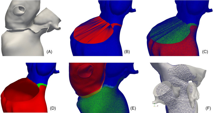
Generation of a fluid‐dynamics mesh of the left heart: (A) the starting internal surfaces of the left ventricle (LV), the left atrium (LA), and the aortic root (AR), divided by a small gap; (B) connecting the LV with the AR; (C) remesh the connection; (D) open the mitral valve ring; (E) connect the LV with the LA and remesh the connection; (F) generate the volumetric mesh

We underline that the connection performed as the first step generates abnormally stretched triangles, but at the same time it creates a cap which perfectly matches with the annulus shape. This demonstrates the robustness of the surface‐connection algorithm and its ability to produce the expected result also when the two rings to be connected vary their distances and are made of a very different number of points. As a final step, like in the other examples, the desired mesh‐size can be defined on the surface and, accordingly, the volumetric mesh can be generated. The example shown in Figure 16F, is made of about 400 K elements. However, for this smooth geometry, coarser or finer meshes can be easily generated by playing with the mesh‐size.

3.4. Examples of numerical simulations

The algorithms proposed in this paper have already provided the baseline of several works concerning the numerical simulation of the cardiac function. In Figure 17 we show some examples of these studies focused on different aspects of the heart modeling:

1. Piersanti et al ⁹¹ proposed new methods for the cardiac fibers generation. In this work electrophysiology simulations on a four‐chambers cardiac geometry were performed, as shown in Figure 17A. This complex mesh has been generated by exploiting most of the proposed algorithms of this paper, especially the ones concerning tagging, connections, and mesh‐size function definition;

2. in their multiscale study of the cardiac active mechanics, Regazzoni et al ⁹² used our algorithms to generate a left‐ventricular mesh for electro‐mechanical simulations, as shown in Figure 17B;

3. Fumagalli et al ²⁸ performed a computational hemodynamics study of the left heart to assess the pathological systolic anterior motion of the mitral valve, as shown in Figure 17C. They used both the harmonic‐connection and harmonic‐extension algorithms in order to connect the patient‐specific ventricle with a template geometry and to extend the image‐based displacement field on the whole domain. They also took advantage of the tagging, mesh‐size and local refinement tools.

FIGURE 17.

Some examples of numerical studies of the cardiac function performed on meshes generated with the tools proposed in this paper: (A) the electrical activation time of an electrophysiology simulation of the whole four‐chambers heart, see Piersanti et al ⁹¹ ; (B) the resulting displacement field at the end of systole of a left‐ventricular electro‐mechanical simulation, see Regazzoni et al ⁹² ; (C) the velocity field at the end of systole of a patient‐specific hemodynamics simulation of the systolic anterior motion of the mitral valve, see Fumagalli et al ²⁸

Moreover, the meshing tools proposed in this paper have also been used in other works regarding the cardiac electrophysiology, ⁹³ , ⁹⁴ the cardiac electromechanics, ⁹⁵ and the cardiac perfusion. ⁹⁶ Finally, we remark that also electro‐mechanics and electro‐mechano‐fluid models of the whole heart are currently under development.

The variety of these numerical studies demonstrates the flexibility of the proposed algorithms that, being connectible with each other into personalized pipelines, can be adapted to the specific needs of different numerical models of the cardiac function.

4. DISCUSSION AND CONCLUSIONS

In this paper, we proposed a set of new algorithms and tools for polygonal surface processing and mesh generation in the context of numerical simulations of the different physical processes that characterize the cardiac function. Our study is motivated by the complexity of the shape of the human heart and by the multi‐physics and multi‐scale cardiac processes that can be simulated numerically. This complexity reverberates in the mesh generation pipeline which, depending on the aspects of the cardiac function to be studied, can consist on a large amount of time‐consuming steps, especially in terms of manpower needed. As a consequence, a general unique pipeline for the cardiac mesh generation is very likely unsuitable, since the procedure strictly depends on the specific cardiac physics or region to be studied. For this reason we proposed various independent algorithms and tools which can be combined in different and flexible ways depending on the specific interest. This allows the creation of ad‐hoc mesh generation pipelines for each cardiac application, ranging from the simplest case of a single physics simulation in a single cardiac chamber to the most complex ones of an electro‐mechano‐fluid model of the whole heart.

We developed our algorithms as an extension of the vascular modeling toolkit (vmtk) library. ⁶⁶ Indeed, we use vmtk both for the already existing algorithms—originally designed for the vascular applications—and for its ability of nesting multiple algorithms in a single pipeline. We presented the algorithms grouping them into four different topics: polygonal surface processing, boundary tags definition, array processing and mesh‐size definition, volumetric mesh processing. We summarize hereafter the main results obtained for each of them.

1. Polygonal surface processing. In order to perform patient‐specific simulations of the cardiac function, a mesh generation pipeline usually starts from unprocessed surfaces reconstructed from medical images. Moreover, the various parts of the heart—for instance the endocardium, the epicardium, or each cardiac chamber—are usually reconstructed separately, producing disconnected or intersecting surfaces. In this context, we proposed three different algorithms to connect separated surfaces into a unique triangulation ready for the volumetric mesh generation:

   1. the surface‐connection algorithm (Section 2.1.1) connects two disconnected surfaces by automatically generating a triangulation between two of their boundary rings. The robustness of the proposed technique is demonstrated in the example of mesh generation pipeline shown in Section 3.3, where we joined the endocardium of the left ventricle with the endocardium of the left atrium and the aortic root (see Figure 16);
   2. the boolean‐connection algorithm (Section 2.1.2) performs boolean operations between intersecting polygonal surfaces by producing, differently than with standard algorithms, ⁸⁰ a regular triangulation ready for the volumetric mesh generation. An example applied to the connection of the left‐ventricular endocardium and epicardium is shown in Section 2.1.2, see also Figure 4.
   3. the harmonic‐connection algorithm (Section 2.1.3) produces a continuous surface by deforming a boundary of an input surface into a boundary of a reference surface and by harmonically extending this deformation on the whole input surface. The conformity of the output triangulation is guaranteed by the internal usage of the surface‐connection algorithm. In Section 2.1.3 we showed the application of this technique to the deformation, at the valvular annulus, of a left‐atrial template geometry into a patient‐specific left‐ventricle, see Figure 5.

We also proposed an algorithm to inflate a surface representing a structure—for example, a cardiac muscle—in order to correct regions where the muscular thickness is unrealistically small (the surface‐thickening algorithm, Section 2.1.4), as shown for the right ventricular outflow tract in Figure 6.

• 2.
  Boundary tags definition. Usually, cardiac boundaries are not sharp edges easy to be localized. Thus, tagging cardiac polygonal surfaces in order to identify specific regions—for instance for the imposition of boundary conditions—is not always a trivial operation. The surface‐tagger tool (Section 2.2) generates tags by exploiting a function defined on it, for instance a distance from an object. In particular, the boundary of the new tag is built at the level where the function assumes a user‐defined value. The resulting tags can have different features depending on the specific algorithm used:

  1. the simple‐array algorithm does not modify the triangulation, by limiting its action to the assignment of a tag to the already existing triangles. Thus, the boundary of the generated tag is typically irregular;
  2. the clip‐array algorithm splits the original triangles into more elements, in order to accurately define the tag exactly at the level where the input function assumes the user‐defined value. Thus, this algorithm generates irregular triangles and must be followed by a surface remeshing to recover the regularity of the triangulation;
  3. the harmonic‐array algorithm, instead, is a novel approach that moves the points of the triangulation thanks to a harmonic map by ensuring that some of them lie on the user‐defined level of the input function. In this way, the generated tag is accurate and the regularity of the triangulation is preserved.

A comparison of the results of the three algorithms has been graphically reported in Figure 7. Although the harmonic‐array algorithm shares the advantages of both the simple‐array and the clip‐array algorithms without any drawback, the other two algorithms can be used for some mesh‐generation pipelines, like in the example shown in Section 3.2 where they are used to generate on a detailed biventricular geometry the tags of valvular annulus and the papillary muscles, respectively (see Figure 14).

• 3. Array processing and mesh‐size definition. Through the surface‐mesh‐size tool (Section 2.3.3), we defined the mesh‐size as a function of relevant geometric quantities. Additionally, we introduced the flexibility of setting it in a different way on each tag. This allows, for instance, to generate volumetric meshes characterized by small elements only where they are required by the geometric complexity or where the user desires a particular accuracy. An example of this strategy is discussed in Section 3.2 for a detailed biventricular geometry (see Figure 15). In this context, we also proposed new algorithms to manipulate arrays defined on the surface—by the harmonic‐extension algorithm (Section 2.3.1)—or to compute relevant geometric quantities for the heart—by the surface‐thickness algorithm (Section 2.3.2).
• 4. Volumetric mesh processing. Once the mesh‐size is defined on the surface, the volumetric tetrahedral mesh can be generated using well‐known robust algorithms. ⁶² However, additional processing can be required for some applications. For instance, the proposed mesh‐refinement algorithm (Section 2.4.2) performs an a priori local refinement of the mesh near a region of interest, as shown in Figure 16 for a hemodynamics mesh of the left‐heart refined near the mitral valve. We also proposed a possible strategy to exploit the tet‐hex algorithm (Section 2.4.3) in order to generate hexahedral meshes from tetrahedral ones, trying to limit the distortion of the final elements (see Figure 13 for an application to a ventricular geometry). Finally, the proposed mesh‐connection algorithm (Section 2.4.1) is of particular interest for the mesh generation of the whole heart. Indeed, it is able to generate a volumetric mesh between two corresponding tags on the surfaces of two volumetric meshes, as shown in Figure 11 for an idealized geometry. This can be applied, for instance, to the generation of the volumetric meshes of the valvular annulus that connect the ventricles to the atria. In addition, starting from the internal surface of the connected meshes, a conforming mesh for the fluid‐dynamics simulations can be easily generated. Moreover, the tool also assigns a specific tag to each different volume. This feature can help to assign specific physical properties to each region, as it is required by multi‐chambers electro‐mechanical models. ⁴⁵ All these considerations make this algorithm of fundamental importance for the generation of the whole heart mesh, essential for the full electro‐mechano‐fluid model of the cardiac function.

The proposed algorithms have been combined into ad‐hoc pipelines to test them in some complex cardiac applications, like the mesh generation of a fully‐detailed ventricular geometry including the papillary muscles and the trabeculae carneae (Section 3.2) or a complete fluid‐dynamics mesh of the left‐heart (Section 3.3). Moreover, as discussed in Section 3.4, they have already been successfully used in other papers to address a broad range of applications. ²⁸ , ⁹¹ , ⁹² , ⁹³ , ⁹⁴ , ⁹⁵ , ⁹⁶ These examples highlight the flexibility of these tools and their ability to be easily applicable to a large variety of cardiac mesh generations through the building of ad‐hoc application‐dependent pipelines. Despite these pipelines can be made up of many steps, once the procedure for the specific application has been established, it can be automatically applied to large datasets, potentially having a strong impact in clinical studies or in the creation of virtual cohorts of heart models. ⁷³

CONFLICT OF INTEREST

The authors declare no potential conflict of interests.

Fedele M, Quarteroni A. Polygonal surface processing and mesh generation tools for the numerical simulation of the cardiac function. Int J Numer Meth Biomed Engng. 2021;37:e3435. 10.1002/cnm.3435

REFERENCES

- 1. Quarteroni A, Manzoni A, Vergara C. The cardiovascular system: mathematical modelling, numerical algorithms and clinical applications. Acta Numerica. 2017;26:365‐590. [Google Scholar]
- 2. Trayanova NA. Whole‐heart modeling: applications to cardiac electrophysiology and electromechanics. Circ Res. 2011;108(1):113‐128. [DOI] [PMC free article] [PubMed] [Google Scholar]
- 3. Dössel O, Krueger MW, Weber FM, Wilhelms M, Seemann G. Computational modeling of the human atrial anatomy and electrophysiology. Med Biol Eng Comput. 2012;50(8):773‐799. [DOI] [PubMed] [Google Scholar]
- 4. Roberts BN, Yang PC, Behrens SB, Moreno JD, Clancy CE. Computational approaches to understand cardiac electrophysiology and arrhythmias. Am J Physiol Heart Circ Physiol. 2012;303(7):H766‐H783. [DOI] [PMC free article] [PubMed] [Google Scholar]
- 5. Colli Franzone P, Pavarino LF, Scacchi S. Mathematical Cardiac Electrophysiology. MS&A Vol 13. Cham: Springer; 2014. [Google Scholar]
- 6. Chabiniok R, Wang VY, Hadjicharalambous M, et al. Multiphysics and multiscale modelling, data–model fusion and integration of organ physiology in the clinic: ventricular cardiac mechanics. Interface Focus. 2016;6(2):20150083. [DOI] [PMC free article] [PubMed] [Google Scholar]
- 7. Strocchi M, Gsell MA, Augustin CM, et al. Simulating ventricular systolic motion in a four‐chamber heart model with spatially varying robin boundary conditions to model the effect of the pericardium. J Biomech. 2020;101:109645. [DOI] [PMC free article] [PubMed] [Google Scholar]
- 8. Smith N, de Vecchi A, McCormick M, et al. euHeart: personalized and integrated cardiac care using patient‐specific cardiovascular modelling. Interface Focus. 2011;1(3):349‐364. [DOI] [PMC free article] [PubMed] [Google Scholar]
- 9. Pennati G, Corsini C, Hsia TY, Migliavacca F. Computational fluid dynamics models and congenital heart diseases. Front Pediatr. 2013;1:4. [DOI] [PMC free article] [PubMed] [Google Scholar]
- 10. Sun W, Martin C, Pham T. Computational modeling of cardiac valve function and intervention. Annu Rev Biomed Eng. 2014;16:53‐76. [DOI] [PMC free article] [PubMed] [Google Scholar]
- 11. Lopez‐Perez A, Sebastian R, Ferrero JM. Three‐dimensional cardiac computational modelling: methods, features and applications. Biomed Eng Online. 2015;14(1):35. [DOI] [PMC free article] [PubMed] [Google Scholar]
- 12. Morris PD, Narracott A, Tengg‐Kobligk VH, et al. Computational fluid dynamics modelling in cardiovascular medicine. Heart. 2016;102(1):18‐28. [DOI] [PMC free article] [PubMed] [Google Scholar]
- 13. Arevalo HJ, Vadakkumpadan F, Guallar E, et al. Arrhythmia risk stratification of patients after myocardial infarction using personalized heart models. Nat Commun. 2016;7:11437. [DOI] [PMC free article] [PubMed] [Google Scholar]
- 14. Niederer SA, Lumens J, Trayanova NA. Computational models in cardiology. Nat Rev Cardiol. 2019;16(2):100‐111. [DOI] [PMC free article] [PubMed] [Google Scholar]
- 15. Zygote solid 3D heart generation II developement report. Tech. Rep., Zygote Media Group Inc.; 2014.
- 16. Iaizzo PA. Handbook of Cardiac Anatomy, Physiology, and Devices. New York: Springer Science & Business Media; 2009. [Google Scholar]
- 17. Kutzner C, Grubmüller H, De Groot BL, Zachariae U. Computational electrophysiology: the molecular dynamics of ion channel permeation and selectivity in atomistic detail. Biophys J. 2011;101(4):809‐817. [DOI] [PMC free article] [PubMed] [Google Scholar]
- 18. Vázquez M, Arís R, Houzeaux G, et al. A massively parallel computational electrophysiology model of the heart. Int J Numer Methods Biomed Eng. 2011;27(12):1911‐1929. [Google Scholar]
- 19. Pagani S, Manzoni A, Quarteroni A. Numerical approximation of parametrized problems in cardiac electrophysiology by a local reduced basis method. Comput Methods Appl Mech Eng. 2018;340:530‐558. [Google Scholar]
- 20. McDowell KS, Zahid S, Vadakkumpadan F, Blauer J, MacLeod RS, Trayanova NA. Virtual electrophysiological study of atrial fibrillation in fibrotic remodeling. PloS One. 2015;10(2):e0117110. [DOI] [PMC free article] [PubMed] [Google Scholar]
- 21. Nordsletten D, Niederer S, Nash M, Hunter P, Smith N. Coupling multi‐physics models to cardiac mechanics. Prog Biophys Mol Biol. 2011;104(1‐3):77‐88. [DOI] [PubMed] [Google Scholar]
- 22. Regazzoni F, Dedè L, Quarteroni A. Active contraction of cardiac cells: a reduced model for sarcomere dynamics with cooperative interactions. Biomech Model Mechanobiol. 2018;17(6):1663‐1686. [DOI] [PubMed] [Google Scholar]
- 23. Peskin CS. The fluid dynamics of heart valves: experimental, theoretical, and computational methods. Annu Rev Fluid Mech. 1982;14(1):235‐259. [Google Scholar]
- 24. Quaini A, Canic S, Guidoboni G, et al. A three‐dimensional computational fluid dynamics model of regurgitant mitral valve flow: validation against in vitro standards and 3D color Doppler methods. Cardiovasc Eng Technol. 2011;2(2):77‐89. [DOI] [PMC free article] [PubMed] [Google Scholar]
- 25. Fedele M, Faggiano E, Dedè L, Quarteroni A. A patient‐specific aortic valve model based on moving resistive immersed implicit surfaces. Biomech Model Mechanobiol. 2017;16(5):1779‐1803. [DOI] [PubMed] [Google Scholar]
- 26. Masci A, Barone L, Dedè L, et al. The impact of left atrial appendage morphology on stroke risk assessment in atrial fibrillation: a computational fluid dynamics study. Front Physiol. 2018;9:1938. [DOI] [PMC free article] [PubMed] [Google Scholar]
- 27. This A, Boilevin‐Kayl L, Fernández MA, Gerbeau JF. Augmented resistive immersed surfaces valve model for the simulation of cardiac hemodynamics with isovolumetric phases. Int J Numer Methods Biomed Eng. 2020;36(3):e3223. [DOI] [PubMed] [Google Scholar]
- 28. Fumagalli I, Fedele M, Vergara C, et al. An image‐based computational hemodynamics study of the Systolic Anterior Motion of the mitral valve. Comput Biol Med. 2020;123:103922. [DOI] [PubMed] [Google Scholar]
- 29. Sugiura S, Washio T, Hatano A, Okada J, Watanabe H, Hisada T. Multi‐scale simulations of cardiac electrophysiology and mechanics using the University of Tokyo heart simulator. Prog Biophys Mol Biol. 2012;110(2‐3):380‐389. [DOI] [PubMed] [Google Scholar]
- 30. Santiago A, Aguado‐Sierra J, Zavala‐Aké M, et al. Fully coupled fluid‐electro‐mechanical model of the human heart for supercomputers. Int J Numer Methods Biomed Eng. 2018;34(12):e3140. [DOI] [PubMed] [Google Scholar]
- 31. Owen SJ. A survey of unstructured mesh generation technology. IMR. 1998;239:267. [Google Scholar]
- 32. Frey PJ, George PL. Mesh Generation: Application to Finite Elements. New York: ISTE Ltd and John Wiley & Sons; 2008. [Google Scholar]
- 33. Cheng SW, Dey TK, Shewchuk J. Delaunay Mesh Generation. Boca Raton: CRC Press; 2012. [Google Scholar]
- 34. Lo DS. Finite Element Mesh Generation. Boca Raton: CRC Press; 2014. [Google Scholar]
- 35. Zhang YJ. Geometric Modeling and Mesh Generation from Scanned Images. Boca Raton: CRC Press; 2018. [Google Scholar]
- 36. Zhang Y, Bajaj C. Finite Element Meshing for Cardiac Analysis. ICES Technical Report 2004; Univ. of Texas at Austin.
- 37. Burton RA, Plank G, Schneider JE, et al. Three‐dimensional models of individual cardiac histoanatomy: tools and challenges. Ann N Y Acad Sci. 2006;1080:301‐319. [DOI] [PMC free article] [PubMed] [Google Scholar]
- 38. Prassl AJ, Kickinger F, Ahammer H, et al. Automatically generated, anatomically accurate meshes for cardiac electrophysiology problems. IEEE Trans Biomed Eng. 2009;56(5):1318‐1330. [DOI] [PMC free article] [PubMed] [Google Scholar]
- 39. Lamata P, Niederer S, Nordsletten D, et al. An accurate, fast and robust method to generate patient‐specific cubic Hermite meshes. Med Image Anal. 2011;15(6):801‐813. [DOI] [PubMed] [Google Scholar]
- 40. Zhang Y, Liang X, Ma J, et al. An atlas‐based geometry pipeline for cardiac Hermite model construction and diffusion tensor reorientation. Med Image Anal. 2012;16(6):1130‐1141. [DOI] [PMC free article] [PubMed] [Google Scholar]
- 41. Augustin CM, Crozier A, Neic A, et al. Patient‐specific modeling of left ventricular electromechanics as a driver for haemodynamic analysis. Europace. 2016;18(suppl_4):iv121‐iv129. [DOI] [PMC free article] [PubMed] [Google Scholar]
- 42. Gillette K, Prassl A, Neic A, Plank G, Bayer J, Vigmond E. Automatic generation of bi‐ventricular models of cardiac electrophysiology for patient specific personalization using non‐invasive recordings. Paper presented at: 2018 Computing in Cardiology Conference (CinC); Vol 45; September 23‐26, 2018; Maastricht, Netherlands:IEEE:1‐4.
- 43. Lopez‐Perez A, Sebastian R, Izquierdo M, Ruiz R, Bishop M, Ferrero JM. Personalized cardiac computational models: from clinical data to simulation of infarct‐related ventricular tachycardia. Front Physiol. 2019;10:580. [DOI] [PMC free article] [PubMed] [Google Scholar]
- 44. Neic A, Gsell MA, Karabelas E, Prassl AJ, Plank G. Automating image‐based mesh generation and manipulation tasks in cardiac modeling workflows using meshtool. SoftwareX. 2020;11:100454. [DOI] [PMC free article] [PubMed] [Google Scholar]
- 45. Strocchi M, Augustin CM, Gsell MA, et al. A publicly available virtual cohort of four‐chamber heart meshes for cardiac electro‐mechanics simulations. PLoS One. 2020;15(6):e0235145. [DOI] [PMC free article] [PubMed] [Google Scholar]
- 46. This A, Morales HG, Bonnefous O, Fernández MA, Gerbeau JF. A pipeline for image based intracardiac CFD modeling and application to the evaluation of the PISA method. Comput Methods Appl Mech Eng. 2020;358:112627. [Google Scholar]
- 47. Zhang Y, Bajaj C, Sohn BS. 3D finite element meshing from imaging data. Comput Methods Appl Mech Eng. 2005;194(48‐49):5083‐5106. [DOI] [PMC free article] [PubMed] [Google Scholar]
- 48. Zheng Y, Barbu A, Georgescu B, Scheuering M, Comaniciu D. Four‐chamber heart modeling and automatic segmentation for 3‐D cardiac CT volumes using marginal space learning and steerable features. IEEE Trans Med Imaging. 2008;27(11):1668‐1681. [DOI] [PubMed] [Google Scholar]
- 49. Hoogendoorn C, Sebastian R, Rodriguez JF, Lekadir K, Frangi AF. An atlas‐and data‐driven approach to initializing reaction‐diffusion systems in computer cardiac electrophysiology. Int J Numer Methods Biomed Eng. 2017;33(8):e2846. [DOI] [PubMed] [Google Scholar]
- 50. Frangi AF, Rueckert D, Schnabel JA, Niessen WJ. Automatic construction of multiple‐object three‐dimensional statistical shape models: application to cardiac modeling. IEEE Trans Med Imaging. 2002;21(9):1151‐1166. [DOI] [PubMed] [Google Scholar]
- 51. Fonseca CG, Backhaus M, Bluemke DA, et al. The Cardiac Atlas Project—an imaging database for computational modeling and statistical atlases of the heart. Bioinformatics. 2011;27(16):2288‐2295. [DOI] [PMC free article] [PubMed] [Google Scholar]
- 52. Hoogendoorn C, Duchateau N, Sanchez‐Quintana D, et al. A high‐resolution atlas and statistical model of the human heart from multislice CT. IEEE Trans Med Imaging. 2012;32(1):28‐44. [DOI] [PubMed] [Google Scholar]
- 53. Bai W, Shi W, de Marvao A, et al. A bi‐ventricular cardiac atlas built from 1000+ high resolution MR images of healthy subjects and an analysis of shape and motion. Med Image Anal. 2015;26(1):133‐145. [DOI] [PubMed] [Google Scholar]
- 54. Chan CL, Anitescu C, Rabczuk T. Volumetric parametrization from a level set boundary representation with PHT‐splines. Comput‐Aided Des. 2017;82:29‐41. [Google Scholar]
- 55. Urick B, Sanders TM, Hossain SS, Zhang YJ, Hughes TJ. Review of patient‐specific vascular modeling: template‐based isogeometric framework and the case for CAD. Arch Comput Method Eng. 2019;26(2):381‐404. [Google Scholar]
- 56. Xanthos T, Dalivigkas I, Ekmektzoglou KA. Anatomic variations of the cardiac valves and papillary muscles of the right heart. Ital J Anat Embryol. 2011;116(2):111‐126. [PubMed] [Google Scholar]
- 57. Shereen R, Lee S, Salandy S, Roberts W, Loukas M. A comprehensive review of the anatomical variations in the right atrium and their clinical significance. Transl Res Anat. 2019;17:100046. [Google Scholar]
- 58. Wongcharoen W, TSAO HM, MH WU, et al. Morphologic characteristics of the left atrial appendage, roof, and septum: implications for the ablation of atrial fibrillation. J Cardiovasc Electrophysiol. 2006;17(9):951‐956. [DOI] [PubMed] [Google Scholar]
- 59. Löhner R, Parikh P. Generation of three‐dimensional unstructured grids by the advancing‐front method. Int J Numer Method Fluids. 1988;8(10):1135‐1149. [Google Scholar]
- 60. George PL, Seveno É. The advancing‐front mesh generation method revisited. Int J Numer Methods Eng. 1994;37(21):3605‐3619. [Google Scholar]
- 61. Löhner R. Progress in grid generation via the advancing front technique. Eng Comput. 1996;12(3‐4):186‐210. [Google Scholar]
- 62. Si H. TetGen, a Delaunay‐based quality tetrahedral mesh generator. ACM Trans Math Softw. 2015;41(2):11. [Google Scholar]
- 63. Biehler J, Wall W. The impact of personalized probabilistic wall thickness models on peak wall stress in abdominal aortic aneurysms. Int J Numer Methods Biomed Eng. 2018;34(2):e2922. [DOI] [PubMed] [Google Scholar]
- 64. Campos JO, Sundnes J, dos Santos RW, Rocha BM. Effects of left ventricle wall thickness uncertainties on cardiac mechanics. Biomech Model Mechanobiol. 2019;18(5):1415‐1427. [DOI] [PubMed] [Google Scholar]
- 65. Campos J, Sundnes J, Dos Santos R, Rocha B. Uncertainty quantification and sensitivity analysis of left ventricular function during the full cardiac cycle. Philos Trans R Soc A. 2020;378(2173):20190381. [DOI] [PMC free article] [PubMed] [Google Scholar]
- 66. Antiga L, Piccinelli M, Botti L, Ene‐Iordache B, Remuzzi A, Steinman DA. An image‐based modeling framework for patient‐specific computational hemodynamics. Med Biol Eng Comput. 2008;46(11):1097‐1112. [DOI] [PubMed] [Google Scholar]
- 67. Geuzaine C, Remacle JF. Gmsh: a 3‐D finite element mesh generator with built‐in pre‐and post‐processing facilities. Int J Numer Methods Eng. 2009;79(11):1309‐1331. [Google Scholar]
- 68. Schöberl J. NETGEN an advancing front 2D/3D‐mesh generator based on abstract rules. Comput Visualization Sci. 1997;1(1):41‐52. [Google Scholar]
- 69. Blacker TD, Owen SJ, Staten ML, et al. CUBIT Geometry and Mesh Generation Toolkit 15.2 User Documentation. Tech. Rep., Sandia National lab.(SNL‐NM), Albuquerque, NM; 2016.
- 70. Cignoni P, Callieri M, Corsini M, Dellepiane M, Ganovelli F, Ranzuglia G. Meshlab: an open‐source mesh processing tool. Paper presented at: Eurographics Italian Chapter Conference; January 2008; Salerno, Italy:129‐136.
- 71. Schmidt R, Singh K. Meshmixer: an interface for rapid mesh composition. Paper presented at: SIGGRAPH '10: ACM SIGGRAPH 2010 Talks; July 2010:1‐1.
- 72. Hess R. The Essential Blender: Guide to 3D Creation with the Open Source Suite Blender. San Francisco: No Starch Press; 2007. [Google Scholar]
- 73. Niederer S, Aboelkassem Y, Cantwell C, et al. Creation and application of virtual patient cohorts of heart models. Philos Trans R Soc A. 2020;378(2173):20190558. [DOI] [PMC free article] [PubMed] [Google Scholar]
- 74. Thakur A, Banerjee AG, Gupta SK. A survey of CAD model simplification techniques for physics‐based simulation applications. Comput‐Aided Des. 2009;41(2):65‐80. [Google Scholar]
- 75. Antiga L, Ene‐Iordache B, Remuzzi A. Computational geometry for patient‐specific reconstruction and meshing of blood vessels from MR and CT angiography. IEEE Trans Med Imaging. 2003;22(5):674‐684. [DOI] [PubMed] [Google Scholar]
- 76. Antiga L. Patient‐specific modeling of geometry and blood flow in large arteries [PhD thesis]. Politecnico di Milano; 2002.
- 77. Lee DT, Schachter BJ. Two algorithms for constructing a Delaunay triangulation. Int J Comput Inform Sci. 1980;9(3):219‐242. [Google Scholar]
- 78. Schroeder WJ, Lorensen B, Martin K. The Visualization Toolkit: An Object‐Oriented Approach to 3D Graphics. Kitware; 2004. [Google Scholar]
- 79. Bærentzen JA, Aanaes H. Signed distance computation using the angle weighted pseudonormal. IEEE Trans Visualization Comput Graph. 2005;11(3):243‐253. [DOI] [PubMed] [Google Scholar]
- 80. Quammen C, Weigle C, Taylor R. Boolean operations on surfaces in vtk without external libraries. Insight J. 2011;797:1‐12. [Google Scholar]
- 81. Chetverikov D, Svirko D, Stepanov D, Krsek P. The trimmed iterative closest point algorithm. Paper presented at: Object Recognition Supported by User Interaction for Service Robots; Vol 3; August 11‐15, 2002; Quebec City, Canada:IEEE:545‐548.
- 82. Chetverikov D, Stepanov D, Krsek P. Robust Euclidean alignment of 3D point sets: the trimmed iterative closest point algorithm. Image Vis Comput. 2005;23(3):299‐309. [Google Scholar]
- 83. Dziuk G, Elliott CM. Finite element methods for surface PDEs. Acta Numer. 2013;22:289‐396. [Google Scholar]
- 84. Bonito A, Demlow A, Nochetto RH. Finite element methods for the Laplace–Beltrami operator. Handbook of Numerical Analysis. Vol 21. Amsterdam: Elsevier; 2020:1‐103. [Google Scholar]
- 85. Suetens P. Fundamentals of Medical Imaging. Cambridge: Cambridge University Press; 2017. 10.1017/9781316671849. [DOI] [Google Scholar]
- 86. Roney C, Bendikas R, Pashakhanloo F, et al. Constructing a human atrial fibre atlas. Ann Biomed Eng. 2021;49 (1):.233‐250. [DOI] [PMC free article] [PubMed] [Google Scholar]
- 87. Bänsch E. Local mesh refinement in 2 and 3 dimensions. IMPACT Comput Sci Eng. 1991;3(3):181‐191. [Google Scholar]
- 88. Zienkiewicz O, Zhu J. Adaptivity and mesh generation. Int J Numer Method Eng. 1991;32(4):783‐810. [Google Scholar]
- 89. Bathe KJ, Zhang H. A mesh adaptivity procedure for CFD and fluid‐structure interactions. Comput Struct. 2009;87(11‐12):604‐617. [Google Scholar]
- 90. De Santis G, De Beule M, Van Canneyt K, Segers P, Verdonck P, Verhegghe B. Full‐hexahedral structured meshing for image‐based computational vascular modeling. Med Eng Phys. 2011;33(10):1318‐1325. [DOI] [PubMed] [Google Scholar]
- 91. Piersanti R, Africa PC, Fedele M, et al. Modeling cardiac muscle fibers in ventricular and atrial electrophysiology simulations. Comput Methods Appl Mech Eng. 2021;373:113468. 10.1016/j.cma.2020.113468. [DOI] [Google Scholar]
- 92. Regazzoni F, Dedè L, Quarteroni A. Biophysically detailed mathematical models of multiscale cardiac active mechanics. PLOS Comput Biol. 2020;16(10):e1008294. 10.1371/journal.pcbi.1008294. [DOI] [PMC free article] [PubMed] [Google Scholar]
- 93. Stella S, Vergara C, Maines M, et al. Integration of activation maps of epicardial veins in computational cardiac electrophysiology. Comput Biol Med. 2020;127:104047. 10.1016/j.compbiomed.2020.104047. [DOI] [PubMed] [Google Scholar]
- 94. Fresca S, Manzoni A, Dedè L, Quarteroni A. Deep learning‐based reduced order models in cardiac electrophysiology. PLOS ONE. 2020;15(10):e0239416. 10.1371/journal.pone.0239416. [DOI] [PMC free article] [PubMed] [Google Scholar]
- 95. Salvador M, Dede L, Quarteroni A. An intergrid transfer operator using radial basis functions with application to cardiac electromechanics. Comput Mech. 2020;66:491‐511. [Google Scholar]
- 96. Di Gregorio S, Fedele M, Pontone G, et al. A computational model applied to myocardial perfusion in the human heart: from large coronaries to microvasculature. J Comput Phys. 2021;424:109836. 10.1016/j.jcp.2020.109836. [DOI] [Google Scholar]