Enabling forward uncertainty quantification and sensitivity analysis in cardiac electrophysiology by reduced order modeling and machine learning

Abstract

We present a new, computationally efficient framework to perform forward uncertainty quantification (UQ) in cardiac electrophysiology. We consider the monodomain model to describe the electrical activity in the cardiac tissue, coupled with the Aliev‐Panfilov model to characterize the ionic activity through the cell membrane. We address a complete forward UQ pipeline, including both: (i) a variance‐based global sensitivity analysis for the selection of the most relevant input parameters, and (ii) a way to perform uncertainty propagation to investigate the impact of intra‐subject variability on outputs of interest depending on the cardiac potential. Both tasks exploit stochastic sampling techniques, thus implying overwhelming computational costs because of the huge amount of queries to the high‐fidelity, full‐order computational model obtained by approximating the coupled monodomain/Aliev‐Panfilov system through the finite element method. To mitigate this computational burden, we replace the full‐order model with computationally inexpensive projection‐based reduced‐order models (ROMs) aimed at reducing the state‐space dimensionality. Resulting approximation errors on the outputs of interest are finally taken into account through artificial neural network (ANN)‐based models, enhancing the accuracy of the whole UQ pipeline. Numerical results show that the proposed physics‐based ROMs outperform regression‐based emulators relying on ANNs built with the same amount of training data, in terms of both numerical accuracy and overall computational efficiency.

We rely on physics‐based ROMs to speed up sensitivity analysis and forward uncertainty quantification in cardiac electrophysiology. We account for the approximation error with respect to the full order model by means of inexpensive ANN regression models. We show quantitatively that the duration of the refractory period is a key factor for the sustainment of the reentry.

Abbreviations

ANN

artificial neural network

FE

finite element

FOM

full order model

GSA

global sensitivity analysis

MLP

multilayer perceptron

ODE

ordinary differential equation

PDE

partial differential equation

POD

proper orthogonal decomposition

RB

reduced basis

ROM

reduced order model

UQ

uncertainty quantification

1. INTRODUCTION

High‐performance computing has enhanced, in the past decade, organ‐level numerical simulations of the heart, integrating complex multi‐scale phenomena – ranging from the subcellular to the tissue scale – with multi‐physics interactions, such as the electromechanical coupling. ¹ Computational cardiology is nowadays a recognized tool of clinical utility regarding risk stratification, decisions' support and personalized medicine. It relies on physics‐based mathematical models and accurate discretization techniques: the former usually depend on several inputs, that can be either directly measured or indirectly estimated according to experimental data; the latter often requires extremely small mesh sizes and time steps.

Model inputs such as physical and/or geometrical parameters – and more generally speaking problem data – cannot be treated, in this context, as completely known quantities, because of both (i) intrinsic randomness affecting physical processes, and (ii) intra‐subject variability – that is, differences between individuals. ² , ³ , ⁴ , ⁵ , ⁶ Variability and lack of knowledge are the two main causes ¹ of uncertainty – this latter being commonly defined as the confidence by which a quantity can be assigned a value. Whenever interested to move towards data‐model integration, embedding uncertainties carried by subject‐specific features into the computational models, and quantifying their impact on the computed results are crucial steps, thus motivating the application of global sensitivity analysis (GSA) and uncertainty quantification (UQ) techniques to cardiovascular problems. ⁷

In this paper we focus on cardiac electrophysiology, that is, the description of the cardiac electrical activity, ⁸ , ⁹ , ¹⁰ , ¹¹ using the monodomain system coupled with the Aliev‐Panfilov ionic model. Despite the input parameters of these models often have a direct physical interpretation, setting their values can be extremely troublesome. For instance, electrical conductivities are tensor fields depending on tissue anisotropy, induced by the presence of fibers and sheets ¹² ; on the other hand, repolarization properties are not easily measurable and ionic models are extremely sensitive to the values of some of their parameters, thus making some pathological conditions hard to reproduce accurately. More generally speaking, uncertainty might affect any input parameter related to the geometrical configuration of the domain where the model is set, model coefficients, sources, initial and boundary conditions. As a result, quantifying the sources of variability and uncertainty in model inputs is of paramount importance to obtain reliable outputs of clinical interest, such as voltage or activation maps, through the numerical approximation of the cardiac models. The task of forward UQ is that of providing a statistical model consisting of a probability distribution of model outputs as a function of uncertain model inputs, and related statistics of interest. Sensitivity analysis can be used instead, prior to forward UQ, to identify model inputs that have either a dominant influence (and so should be measured as precisely as possible), or a mild effect (in which case uncertainty in those inputs may be neglected) on a given output. Even if this work focuses on UQ, we highlight that this latter is only one of the three pillars – verification, validation, and uncertainty quantification – providing the so‐called VVUQ framework, aiming at improving processes in computational science. Verification and validation of models in cardiac electrophysiology, however, are beyond the scope of the present work.

UQ and sensitivity analysis entail tremendous computational costs because of the need to rely on stochastic sampling (e.g., Monte Carlo or quasi Monte Carlo) techniques, ¹³ requiring a large number of queries to the state problem (given in our case by a nonlinear, time‐dependent, coupled PDE‐ODEs system). To improve the performances we can follow different strategies such as, (i) replacing computationally expensive high‐fidelity full‐order models (FOMs) with computationally inexpensive surrogate or reduced‐order models (ROMs), (ii) to improve sampling procedures exploiting, for example, (adaptive) sparse grid, ¹⁴ , ¹⁵ , ¹⁶ multi‐level or multi‐fidelity ¹⁷ Monte Carlo techniques ¹⁸ , ¹⁹ or (iii) to adopt different stochastic procedures, ²⁰ such as stochastic Galerkin and stochastic collocation methods. ²¹ , ²² In this paper we focus on the first strategy for its ease of implementation and flexibility.

Among surrogate models, several options are available, such as (i) data fits or emulators, obtained via artificial neural network (ANN) regression, ²³ polynomial chaos expansions ²⁴ or Gaussian process regression, ²⁵ that directly approximates the input–output mapping by fitting an emulator to a set of training data – that is, a set of inputs and corresponding outputs obtained from model runs; (ii) lower‐fidelity models, introducing modeling simplifications (e.g., coarser meshes or simplified physics, such as the Eikonal or reaction‐Eikonal models ²⁶ ); and (iii) ROMs obtained through a projection process on the equations governing the FOM to reduce the state‐space dimensionality. Although typically more intrusive to implement, ROMs often yield more accurate approximations than data fits and usually generate more significant computational gains than lower‐fidelity models, requiring less training data. Since we are interested to deal with complex depolarization and repolarization patterns including sustained or non‐sustained reentries, we avoid using simplified physical models, because they might fail in describing such complex patterns. ²⁶ , ²⁷ We instead compare data fits and projection‐based ROMs when dealing with sensitivity analysis and forward UQ. In particular, we assess the effect of parameters (and related uncertainty) on tissue activation patterns and tissue refractoriness, leading to sustained and non‐sustained reentry waves. Despite several works have proposed computational models to enhance understanding of cardiac arrhythmias, focusing on both two‐dimensional geometries ²⁸ , ²⁹ , ³⁰ , ³¹ , ³² and three‐dimensional, patient‐specific configurations, ³³ , ³⁴ , ³⁵ , ³⁶ uncertainty propagation in these applications has been seldom taken into account systematically; we mention, for example, Reference 6 for the estimation of the local tissue excitability of a cardiac electrophysiological model and Reference 37 for the quantification of the uncertainty about the shape of the left atrium derived from cardiac magnetic resonance images. On the other hand, several works have focused on the way uncertainty can be quantified and propagated within single‐cell models. ⁴ , ³⁸

In this paper, we propose a novel, physics‐based computational pipeline to perform global sensitivity analysis and forward UQ in cardiac electrophysiology, aiming at investigating the effect of model parameters (related with both the stimulation protocol and the ionic activity) on complex patterns including spiral waves reentry, simulating the presence of tachycardia. Our framework features several novelties compared to existing literature:

• First of all, we exploit efficient and accurate ROMs built through the reduced basis (RB) method for parametrized PDEs as physics‐based surrogate models to speed up our UQ analysis, rather than data fits or emulators. In this way, we reduce the computational complexity entailed by stochastic sampling approaches by relying on less expensive queries to the full‐order state problem, still preserving the fidelity of an accurate model such as the monodomain equation.

• Moreover, we properly account for the approximation error with respect to the FOM – which can also be seen as a form of simulator uncertainty – by means of inexpensive ANN regression models. Then, we perform a variance‐based global sensitivity analysis, taking into account the simultaneous variation of multiple parameters and their possible interactions.

• Furthermore, we propagate uncertainty from the most relevant inputs (among several parameters affecting the ionic model, the coefficients and data of the monodomain model) to outputs of interest related with the activation map.

• Finally, we show that a purely data‐driven emulator of the input–output map, built through an ANN regression model, does not ensure the same accuracy reached by the proposed physics‐based ROM strategy.

The structure of the paper is as follows. In Section 2 we formulate the monodomain system coupled with the Aliev‐Panfilov ionic model, the high‐fidelity FOM, and an efficient ROM based on the POD‐Galerkin method. Moreover, we show how to take advantage of the proposed ANN and ROM strategies to perform variance‐based GSA and forward UQ. In Section 3 we assess the computational performances of the proposed methods on a two‐dimensional benchmark problem, where the parameters of interest are related to the stimulation protocol and the ionic activity. A discussion on the obtained numerical results, and a comparison with existing literature, are reported in Section 4, followed by some Conclusions in Section 5.

2. METHODS

After formulating the problem we focus on, we show how to solve it efficiently through an efficient ROM. Then, we recall some fundamentals in sensitivity analysis and forward UQ, showing how reduction errors propagate through the forward UQ process.

2.1. State problem, input uncertainties and outputs of interest

Mathematical models of cardiac electrophysiology describe the action‐potential mechanism of depolarization and repolarization of cardiac cells, which consists in a rapid variations of the cell membrane electric potential with respect to a resting potential. Indeed, the generation of ionic currents at the microscopic scale through the cellular membrane produces a local action potential, which is propagated, at the macroscopic scale, from cell to cell, in the form of a trans‐membrane potential. This latter is described by means of PDEs – the bidomain model, or the simplified monodomain model – suitably coupled with ODEs modeling the ionic currents in the cells. Several ionic models have been investigated in the past decades, either providing a phenomenological description of the action potential disregarding sub‐cellular processes (such as the Rogers‐McCulloch, Aliev‐Panfilov, Bueno‐Orovio models), or allowing explicit description of the kinetics of different ionic currents (see, e.g., ⁸ , ¹⁰ , ³⁹ ).

Throughout the paper, $\mathit{\mu }\in \mathcal{P}$ will denote an input parameter vector, whose components might represent physical and/or geometrical features affecting the coupled ODE‐PDE model; $\mathcal{P}\subset {\mathrm{ℝ}}^p$ will denote the parameter space. Here we are interested to quantify the uncertainty in the evolution of the electric potential for a range of physical parameters affecting both electric conductivities at the tissue level and the ionic dynamics at the cellular scale. The state problem is obtained by coupling the monodomain model for the (dimensionless ² ) transmembrane potential u(μ) with a ionic model – here involving a single gating variable w(μ) – in a domain Ω ⊂ ℝ^d, d = 2, 3, representing, for example, a portion of the myocardium.

This results in the following time‐dependent nonlinear diffusion–reaction problem: for each t ∈ (0, T),

$$\begin{array}{rr}\frac{\partial u\left(\mathit{\mu }\right)}{\partial t}-\mathrm{div}\left(\mathbf{D}\left(\mathit{\mu }\right)\nabla u\left(\mathit{\mu }\right)\right)+I_{\mathit{ion}}\left(u\left(\mathit{\mu }\right),w\left(\mathit{\mu }\right);\mathit{\mu }\right)=I_{\mathit{app}}\left(\mathit{\mu }\right)& \text{in}\mathrm{\Omega }\\ \frac{\partial w\left(\mathit{\mu }\right)}{\partial t}+g\left(u\left(\mathit{\mu }\right),w\left(\mathit{\mu }\right);\mathit{\mu }\right)=0& \text{in}\mathrm{\Omega }\\ \frac{\partial u\left(\mathit{\mu }\right)}{\partial n}=0& \mathrm{on}\mathrm{\partial \Omega }\\ u\left(0;\mathit{\mu }\right)=u_0,w\left(0;\mathit{\mu }\right)=w_0.& \end{array}$$ (1)

Here t denotes a rescaled time, I _app is an applied current providing the (initial) activation of the tissue, while the reaction term I _ion and the function g both depend on u and w, thus making the PDE and the ODEs system two‐ways coupled. The diffusivity tensor D depends on the fibers‐sheets structure of the tissue, and affects conduction velocities and directions. Among several possible choices of ionic models, we consider the Aliev‐Panfilov model, for which

$$I_{\mathit{ion}}\left(u,w\right)=\mathit{Ku}\left(u-a\right)\left(u-1\right)+\mathit{wu},g\left(u,w\right)=\left({\epsilon }_0+\frac{c_{1}w}{c_2+u}\right)\left(-w-\mathit{Ku}\left(u-b-1\right)\right);$$ (2)

the coefficients K, a, b, ε ₀, c ₁, c ₂ are related to the cell.

2.2. High‐fidelity, full‐order model

We consider the Galerkin finite element (FE) method as high‐fidelity FOM. To this goal, problem (1) is first discretized in space using linear finite elements for the transmembrane potential; the number of degrees of freedom related to the spatial discretization is denoted by N _h and corresponds in this case to the number of mesh vertices. The time interval [0, T] is partitioned in N _t = T/Δt time steps, t ^(k) = kΔt, k = 0, …, N _t, and a semi‐implicit, first order, one‐step scheme is then used for time discretization ⁴¹ ; the nonlinear term $I_{\mathit{ion}}\in {\mathrm{ℝ}}^{N_h}$ at each time t ^(k + 1) is then evaluated at the solution already computed at time t ^(k). At each time step t ^(k), k = 1, …, N _t, a system of N _h (independent) nonlinear equations must then be solved, arising from the backward (implicit) Euler method: given w ⁰(μ) = w ₀(μ), solve

$${\mathbf{w}}^{\left(k+1\right)}\left(\mathit{\mu }\right)-\mathrm{\Delta }t\mathbf{g}\left({\mathbf{u}}^{\left(k\right)}\left(\mathit{\mu }\right),{\mathbf{w}}^{\left(k+1\right)}\left(\mathit{\mu }\right);\mathit{\mu }\right)={\mathbf{w}}^{\left(k\right)}\left(\mathit{\mu }\right),k=0,\dots ,N_t-1.$$ (3)

The so‐called ionic current interpolation strategy is used to evaluate the ionic current term, so that only the nodal values are used to build a (piecewise linear) interpolant of the ionic current. This yields a sequence in time of μ‐dependent linear systems,

$$\left(\frac{\mathbb{M}\left(\mathit{\mu }\right)}{\mathrm{\Delta }t}+\mathbb{A}\left(\mathit{\mu }\right)\right){\mathbf{u}}^{\left(k+1\right)}\left(\mathit{\mu }\right)+{\mathbf{I}}_{\mathit{ion}}\left({\mathbf{u}}^{\left(k\right)}\left(\mathit{\mu }\right),{\mathbf{w}}^{\left(k+1\right)}\left(\mathit{\mu }\right);\mathit{\mu }\right)=\frac{\mathbb{M}\left(\mathit{\mu }\right)}{\mathrm{\Delta }t}{\mathbf{u}}^{\left(k\right)}\left(\mathit{\mu }\right)+{\mathbf{I}}_{\mathit{app}}^{\left(k+1\right)}\left(\mathit{\mu }\right),k=0,\dots ,N_t-1,$$ (4)

where ${\mathbf{u}}^{\left(k\right)}\left(\mathit{\mu }\right)\in {\mathrm{ℝ}}^{N_h}$ and ${\mathbf{w}}^{\left(k\right)}\left(\mathit{\mu }\right)\in {\mathrm{ℝ}}^{N_h}$ denote the FOM vector representation of the transmembrane potential and the state variables, respectively, at time t ^(k). The vectors ${\mathbf{u}}^0={\mathbf{u}}_0\left(\mathit{\mu }\right)\in {\mathrm{ℝ}}^{N_h}$, ${\mathbf{w}}^0={\mathbf{w}}_0\left(\mathit{\mu }\right)\in {\mathrm{ℝ}}^{N_h}$ provide instead the initial conditions. Here $\mathbb{M}\left(\mathit{\mu }\right)\in {\mathrm{ℝ}}^{N_h\times N_h}$ denotes the mass matrix, $\mathbb{A}\left(\mathit{\mu }\right)\in {\mathrm{ℝ}}^{N_h\times N_h}$ encodes the diffusion operator appearing in the monodomain equation, whereas ${\mathbf{I}}_{\mathit{app}}^{\left(k+1\right)}\in {\mathrm{ℝ}}^{N_h}$ encodes the applied current at time t ^(k + 1).

The major computational costs are entailed by assembling the terms I _ion and g at each time step and by the solution of the linear system (4); indeed, extremely small spatial mesh sizes h and time steps Δt must be chosen to capture the fast propagation of sharp (and, possibly, μ‐dependent) moving fronts correctly, ²⁹ , ⁴² , ⁴³ thus yielding an extremely large dimension N _h.

2.3. Reduced‐order models for parametrized systems

To speed up the solution of the state problem (1) and make both GSA and UQ feasible for the application at hand, we rely on the reduced basis (RB) method for parametrized PDEs. This technique performs a Galerkin projection onto low‐dimensional subspaces built from a set of snapshots of the high‐fidelity FOM, by, for example, the Proper Orthogonal Decomposition (POD) technique. We refer to the resulting projection‐based ROM as to POD‐Galerkin ROM. In this case, snapshots are obtained by FOM solutions calculated for different values of the parameters (selected through Latin hypercube sampling), at different time steps. Then, suitable hyper‐reduction techniques, such as the Discrete Empirical Interpolation Method (DEIM) ⁴⁴ and its matrix version MDEIM, ⁴⁵ allow us to efficiently handle nonlinear and parameter‐dependent terms. ⁴⁶ , ⁴⁷

For the sake of brevity, here we only sketch the main aspects involved in the RB approximation of the problem at hand. Regarding the PDE system (4), we assume that the RB approximation of the transmembrane potential at time t ^(k) is expressed by a linear combination of the RB basis functions,

$${\mathbf{u}}^{\left(k\right)}\left(\mathit{\mu }\right)\approx \mathbb{V}{\mathbf{u}}_n^{\left(k\right)}\left(\mathit{\mu }\right),$$ (5)

where $\mathbb{V}\in {\mathrm{ℝ}}^{N_h\times n}$ collects the (degrees of freedom of the) reduced basis functions. In the case of POD, $\mathbb{V}$ is made by the first n singular vectors of the snapshot matrix $\mathbf{S}=\left[{\mathbf{u}}^{\left(1\right)}\left({\mu }_1\right)|\dots |{\mathbf{u}}^{\left(N_t\right)}\left({\mu }_1\right)|\dots |\dots {\mathbf{u}}^{\left(1\right)}\left({\mu }_{N_{\mathit{\text{snap}}}}\right)|\dots |{\mathbf{u}}^{\left(1N_t\right)}\left({\mu }_{N_{\mathit{\text{snap}}}}\right)\right]$.

After updating the state variables to its current value w ^(k + 1)(μ) at time t ^(k + 1) by solving (3), the Galerkin‐RB problem reads as:

$$\left(\frac{{\mathbb{M}}_n\left(\mathit{\mu }\right)}{\mathrm{\Delta }t}+{\mathbb{A}}_n\left(\mathit{\mu }\right)\right){\mathbf{u}}_n^{\left(k+1\right)}+{\mathbb{V}}^T{\mathbf{I}}_{\mathit{ion}}\left(\mathbb{V}{\mathbf{u}}_n^{\left(k\right)},{\mathbf{w}}^{\left(k+1\right)};\mathit{\mu }\right)=\frac{{\mathbb{M}}_n\left(\mathit{\mu }\right)}{\mathrm{\Delta }t}{\mathbf{u}}_n^{\left(k\right)}+{\mathbf{I}}_{\mathit{app}}^{\left(k+1\right)}\left(\mathit{\mu }\right),k=0,\dots ,N_t-1,$$

where ${\mathbb{A}}_n\left(\mathit{\mu }\right)={\mathbb{V}}^T\mathbb{A}\left(\mathit{\mu }\right)\mathbb{V}$ and ${\mathbb{M}}_n\left(\mathit{\mu }\right)={\mathbb{V}}^T\mathbb{M}\left(\mathit{\mu }\right)\mathbb{V}$. Since the μ‐dependence shown by these matrices is nonaffine, we rely on MDEIM to get an approximate affine expansion. Then, we can take advantage of DEIM to avoid the evaluation of the full‐order array ${\mathbf{I}}_{\mathit{ion}}\in {\mathrm{ℝ}}^{N_h}$ and preserve the overall ROM efficiency. We thus approximate

$${\mathbf{I}}_{\mathit{ion}}\left(\mathbb{V}{\mathbf{u}}_n^{\left(k\right)},{\mathbf{w}}_h^{\left(k+1\right)};\mathit{\mu }\right)\approx {\tilde{\mathbf{I}}}_{\mathit{ion}}\left(\mathit{\mu }\right)=\sum _{q=1}^m{\theta }_q\left(t^{\left(k\right)};\mathit{\mu }\right){\mathbf{z}}_q$$

once m ≪ N _h μ‐independent vectors ${\mathbf{z}}_q\in {\mathrm{ℝ}}^{N_h}$, 1 ≤ q ≤ m basis vectors have been calculated, from a set of N _snap ⋅ N _t snapshots $\left\{{\mathbf{I}}_{\mathit{ion}}\left(\mathbb{V}{\mathbf{u}}_n^{\left(k\right)}\left({\mathit{\mu }}^k\right),{\mathbf{w}}_h^{\left(k+1\right)}\left({\mathit{\mu }}^k\right);{\mathit{\mu }}^k\right),k=1,\dots ,N_{\mathit{\text{snap}}},\mathrm{\ell }=0,\dots ,N_t-1\right\}$; the μ‐dependent weights ${\theta }_q:\mathcal{P}\mapsto \mathrm{ℝ}$ are then computed by imposing m interpolation constraints. Basis vectors are computed by means of POD, ⁴⁴ whereas the set of points (in the physical domain) where interpolation constraints are imposed are iteratively selected by employing the so‐called magic points algorithm. ⁴⁸ , ⁴⁹ The ionic term in the potential equation can be thenapproximated by

$${\mathbb{V}}^T{\mathbf{I}}_{\mathit{ion}}\left(\mathbb{V}{\mathbf{u}}_n^{\left(k\right)}\left(\mathit{\mu }\right),{\mathbf{w}}^{\left(k+1\right)}\left(\mathit{\mu }\right);\mathit{\mu }\right)\approx \underset{N_h\times m}{\underbrace{{\mathbb{V}}^T\mathbf{\Phi }{\left({\mathrm{\mathbb{P}}}^T\mathbf{\Phi }\right)}^{-1}}}\underset{m\times 1}{\underbrace{{\mathbf{I}}_{\mathit{ion}}\left({\mathrm{\mathbb{P}}}^T\mathbb{V}{\mathbf{u}}_n^{\left(k\right)}\left(\mathit{\mu }\right),{\mathrm{\mathbb{P}}}^T{\mathbf{w}}^{\left(k+1\right)}\left(\mathit{\mu }\right);\mathit{\mu }\right)}}$$

where $\mathbf{\Phi }=\left[{\mathbf{z}}_1|\dots |{\mathbf{z}}_m\right]\in {\mathrm{ℝ}}^{N_h\times m}$ and $\mathrm{\mathbb{P}}=\left[{\mathbf{e}}_{{\mathrm{ℐ}}_1}|\dots |{\mathbf{e}}_{{\mathrm{ℐ}}_m}\right]\in {\mathrm{ℝ}}^{N_h\times m}$, with ${\mathbf{e}}_{{\mathrm{ℐ}}_i}={\left[0,\dots ,\mathrm{0,1,0},\dots ,0\right]}^T\in {\mathrm{ℝ}}^{N_h}$, being ℐ the set of m interpolation indices ℐ ⊂ {1, ⋯, N _h}, with ∣ℐ ∣  = m. Note that the matrix ${\mathrm{\Phi }}_m={\mathbb{V}}^T\mathbf{\Phi }{\left({\mathrm{\mathbb{P}}}^T\mathbf{\Phi }\right)}^{-1}$ is μ‐independent and can be assembled once for all. This way of proceeding also enhances the solution of the ODE system (3). Indeed, only m components ℐ₁, …, ℐ_m must be advanced in time, thus resulting in a reduced ODEs system for the vector ${\mathbf{w}}_m^{\left(k\right)}={\mathrm{\mathbb{P}}}^T{\mathbf{w}}^{\left(k\right)}\in {\mathrm{ℝ}}^m$.

Finally, the ROM for the monodomain system (1) reads as: given $\mathit{\mu }\in \mathcal{P}$, find $\left({\mathbf{u}}_n^{\left(k+1\right)}\left(\mathit{\mu }\right),{\mathbf{w}}_m^{\left(k+1\right)}\left(\mathit{\mu }\right)\right)\in {\mathrm{ℝ}}^{N_h}\times {\mathrm{ℝ}}^m$ such that ${\mathbf{u}}_n^0\left(\mathit{\mu }\right)={\mathbb{V}}^T$ u ₀(μ), ${\mathbf{w}}_m^0={\mathrm{\mathbb{P}}}^T{\mathbf{w}}_0\left(\mathit{\mu }\right)$, and, for k = 0, …, N _t − 1,

$$\begin{array}{ll}{\mathbf{w}}_m^{\left(k+1\right)}\left(\mathit{\mu }\right)-\mathrm{\Delta }t\mathbf{g}\left({\mathrm{\mathbb{P}}}^T\mathbb{V}{\mathbf{u}}_n^{\left(k\right)}\left(\mathit{\mu }\right),{\mathbf{w}}_m^{\left(k+1\right)}\left(\mathit{\mu }\right);\mathit{\mu }\right)={\mathbf{w}}_h^{\left(k\right)}\left(\mathit{\mu }\right),& \\ \left(\frac{{\mathbb{M}}_n\left(\mathit{\mu }\right)}{\mathrm{\Delta }t}+{\mathbb{A}}_n\left(\mathit{\mu }\right)\right){\mathbf{u}}_n^{\left(k+1\right)}\left(\mathit{\mu }\right)+{\mathrm{\Phi }}_m{\mathbf{I}}_{\mathit{ion}}\left({\mathrm{\mathbb{P}}}^T\mathbb{V}{\mathbf{u}}_n^{\left(k\right)}\left(\mathit{\mu }\right),{\mathbf{w}}_m^{\left(k+1\right)}\left(\mathit{\mu }\right);\mathit{\mu }\right)=\frac{{\mathbb{M}}_n\left(\mathit{\mu }\right)}{\mathrm{\Delta }t}{\mathbf{u}}_n^{\left(k\right)}\left(\mathit{\mu }\right)+{\mathbb{V}}^T{\mathbf{I}}_{\mathit{app}}^{\left(k+1\right)}\left(\mathit{\mu }\right).& \end{array}$$

Despite several works have exploited POD‐Galerkin ROMs for the simulation of the cardiac function, ⁵⁰ , ⁵¹ , ⁵² , ⁵³ , ⁵⁴ for the sake of computational efficiency here we consider a generalization of the usual POD approach, requiring the construction of local RB spaces, as proposed in Reference 47. In this respect, clustering algorithms, such as the k‐means algorithm, are employed, prior to performing POD, to partition snapshots (of both the solution to the parametrized coupled monodomain‐ionic model (1), and the nonlinear terms) into N _c clusters, for a chosen number N _c ≥ 1; then, a local reduced basis is built for each cluster through POD. ⁵⁵

For instance, in the case of solution snapshots, we employ k‐means to partition the columns of S into N _c submatrices $\left\{{\mathbf{S}}^1,\dots ,{\mathbf{S}}^{N_c}\right\}$ in order to minimize the distance between each vector in the cluster and the cluster sample mean. In other words, the objective is to find:

$$\left\{{\mathbf{S}}_u^1,\dots ,{\mathbf{S}}_u^{N_c}\right\}=\arg \underset{{\mathbf{S}}_u}{\min }\sum _{\mathrm{\ell }=1}^{N_c}\sum _{\mathbf{u}\in {\mathbf{S}}_u^{\mathrm{\ell }}}\parallel \mathbf{u}-{\mathbf{c}}^{\mathrm{\ell }}{\parallel }^2,{\mathbf{c}}^{\mathrm{\ell }}=\frac{1}{\mid {\mathbf{S}}_u^{\mathrm{\ell }}\mid }\sum _{\mathbf{u}\in {\mathbf{S}}_u^{\mathrm{\ell }}}\mathbf{u},\mathrm{\ell }=1,\dots ,N_c,$$

before computing the POD basis. Here, ${\left\{{\mathbf{c}}^{\mathrm{\ell }}\right\}}_{\mathrm{\ell }=1}^{N_c}$ are the so‐called centroids (i.e., the cluster centers) selected by the k‐means algorithm. Then, when solving the ROM, the local basis $\overline{\mathrm{\ell }}$ is selected at each time step k = 0, …, N _t − 1 with respect to the current solution of the system ${\mathbf{Vu}}_n^{\left(k\right)}\left(\mathit{\mu }\right)$ by minimizing the distance between ${\mathbf{Vu}}_n^{\left(k\right)}\left(\mathit{\mu }\right)$ and the centroids, that is, $\overline{\mathrm{\ell }}=\arg {\min }_{\mathrm{\ell }}\parallel {\mathbf{Vu}}_n^{\left(k\right)}\left(\mathit{\mu }\right)-{\mathbf{c}}^{\mathrm{\ell }}{\parallel }^2$. It is possible to show (see Reference 47) that this latter task can be performed inexpensively only relying on the ROM arrays. A similar procedure is then applied for the construction of local bases to treat nonlinear terms through the DEIM.

We highlight that more sophisticated bioelectrical activity models (e.g., ten Tusscher‐Panfilov, O'Hara‐Rudy, or others) with many state variables would not impact on the construction of the ROM dramatically. In those cases, the ROM would result even more efficient compared to the FOM, due to the large number of ODEs this latter would involve. This is due to the use of the ionic current interpolation, and to the fact that the DEIM only requires to evaluate ionic variables at a set of few, selected points in the domain, thus requiring the solution of few ODEs during the online stage.

2.4. Sensitivity analysis and forward uncertainty quantification

Hereon, we assume that μ is a vector‐valued random variable (or random vector), whose support is $\mathcal{P}={\mathcal{P}}_1\times \dots \times {\mathcal{P}}_p$, being ${\mathcal{P}}_i\subseteq \mathrm{ℝ}$, i = 1, …, p, enabling us to parametrize uncertain inputs of the ODE‐PDE system; we denote by π(μ) the probability density function (pdf) of μ. For the sake of simplicity, we consider all the parameters normalized in the range [0, 1]. Therefore, the (approximated) solution of this latter system, u _h(t; μ), is itself a random function of a random vector, besides spatial coordinates and time. In addition, we denote by $y_h\left(\mathit{\mu }\right)=\mathcal{Q}\left(u_h\left(t;\mathit{\mu }\right)\right)\in \mathrm{ℝ}$ some (random) output Quantities of Interest (QoI) we want to evaluate, which depends by the random input μ through the state variable u _h.

Because of the dependence on u _h, the pdf of y _h cannot be determined in closed form; therefore, we need to draw samples from its distribution, and to compute statistics such as its expected value and its variance

$$\mathbb{E}\left[y_h\right]={\int }_{\mathcal{P}}{y}_h\left(\mathit{\mu }\right)\pi \left(\mathit{\mu }\right)d\mathit{\mu },\mathrm{Var}\left(y_h\right)={\int }_{\mathcal{P}}{\left(y_h\left(\mathit{\mu }\right)-\mathbb{E}\left[y_h\right]\right)}^2\pi \left(\mathit{\mu }\right)d\mathit{\mu }={\int }_{\mathcal{P}}{\left(y_h\left(\mathit{\mu }\right)\right)}^2\pi \left(\mathit{\mu }\right)d\mathit{\mu }-\mathbb{E}{\left[y_h\right]}^2.$$

With this aim, we rely on Monte Carlo (MC) methods, which provide an approximation to $\mathbb{E}\left[y_h\right]$ and Var(y _h) exploiting a random sample {μ _q}, q = 1, …, N _mc, drawn from the distribution of μ, as follows:

$$\mathbb{E}\left[y_h\right]\approx \frac{1}{N_{\mathit{mc}}}\sum _{q=1}^{N_{\mathit{mc}}}{y}_h\left({\mathit{\mu }}_q\right),\mathrm{Var}\left(y_h\right)\approx \frac{1}{N_{\mathit{mc}}-1}\sum _{q=1}^{N_{\mathit{mc}}}{\left(y_h\left({\mathit{\mu }}_q\right)-\frac{1}{N_{\mathit{mc}}}\sum _{q=1}^{N_{\mathit{mc}}}{y}_h\left({\mathit{\mu }}_q\right)\right)}^2.$$ (5)

We also need to compute conditional expectations and conditional variances when dealing with variance‐based sensitivity analysis, since the sensitivities of the output with respect to the parameters are measured by looking at the amount of variance caused by the parameter μ _i, i = 1, …, p. Indeed, assume to fix the parameter μ _i at a particular value ${\mu }_i^{*}$, and let ${\mathrm{Var}}_{{\mathit{\mu }}_{\sim i}}\left(y_h|{\mu }_i={\mu }_i^{*}\right)$ be the resulting variance of y _h, taken over μ _∼i (all parameters but μ _i). We call this a conditional variance, as it is conditional on μ _i being fixed to ${\mu }_i^{*}$, and can use it as a measure of the relative importance of μ _i – the smaller ${\mathrm{Var}}_{{\mathit{\mu }}_{\sim i}}\left(y_h|{\mu }_i={\mu }_i^{*}\right)$, the greater the influence of μ _i on the QoI. To make this measure independent of ${\mu }_i^{*}$, we average it over all possible values ${\mu }_i^{*}$, obtaining

$${\mathbb{E}}_{{\mu }_i}\left[{\mathrm{Var}}_{{\mathit{\mu }}_{\sim i}}\left(y_h|{\mu }_i\right)\right]={\int }_{{\mathcal{P}}_i}{\mathrm{Var}}_{{\mathit{\mu }}_{\sim i}}\left(y_h|{\mu }_i\right){\pi }_i\left({\mu }_i\right)d{\mu }_i,i=1,\dots ,p,$$ (6)

which we also refer to as residual variance. According to the law of total variance (or variance decomposition formula),

$$\mathrm{Var}\left(y_h\right)={\mathrm{Var}}_{{\mu }_i}\left({\mathbb{E}}_{{\mathit{\mu }}_{\sim i}}\left[y_h|{\mu }_i\right]\right)+{\mathbb{E}}_{{\mu }_i}\left[{\mathrm{Var}}_{{\mathit{\mu }}_{\sim i}}\left(y_h|{\mu }_i\right)\right],i=1,\dots ,p.$$ (7)

The first term at the right hand side is the so‐called explained variance, that is, the variance (with respect to μ _i) of the conditional expectation

$${\mathbb{E}}_{{\mathit{\mu }}_{\sim i}}\left[y_h|{\mu }_i\right]={\int }_{\mathcal{P}}{y}_h\left(\mathit{\mu }\right){\pi }_{{\mathit{\mu }}_{\sim i}}\left(\mathit{\mu }|{\mu }_i\right)d\mathit{\mu }i=1,\dots ,p,$$

that is,

$${\mathrm{Var}}_{{\mu }_i}\left({\mathbb{E}}_{{\mathit{\mu }}_{\sim i}}\left[y_h|{\mu }_i\right]\right)={\int }_{{\mathcal{P}}_i}{\left({\mathbb{E}}_{{\mathit{\mu }}_{\sim i}}\left[y_h|{\mu }_i\right]\right)}^2{\pi }_i\left({\mu }_i\right)d{\mu }_i-{\left({\int }_{{\mathcal{P}}_i}{\mathbb{E}}_{{\mathit{\mu }}_{\sim i}}\left[y_h|{\mu }_i\right]{\pi }_i\left({\mu }_i\right)d{\mu }_i\right)}^2.$$ (8)

This term thus represents the reduction of the variance in the output QoI due to the knowledge of μ _i. We have denoted by ${\pi }_{{\mathit{\mu }}_{\sim i}}\left(\mathit{\mu }|{\mu }_i\right)$ the conditional pdf of μ given μ _i, defined as ${\pi }_{{\mathit{\mu }}_{\sim i}}\left(\mathit{\mu }|{\mu }_i\right)=\pi \left(\mathit{\mu }\right)/{\pi }_i\left({\mu }_i\right)$, having assumed that the parameter components μ ₁, …, μ _p are independent; here π _i(μ _i) denotes the marginal pdf of μ _i. Also to compute the conditional expectation and its variance we will rely on MC methods, see Section 2.4.1.

2.4.1. Variance‐based global sensitivity analysis

Sensitivity analysis quantifies the effects of parameter variation on the output QoI, providing a criterium to rank the most influential input parameters. ⁵⁶ In this work we consider a variance‐based global sensitivity analysis (GSA) which describes the amount of output variance generated from the variation of any single parameter, and also from interactions among parameters. ⁵⁷ In this setting, input parameters ranking is based on which input, if fixed to its true value, yields the largest expected reduction in output QoI uncertainty. Compared to the elementary effect method, which computes the effect associated with changes in the ith parameter by changing one parameter at a time, variance‐based GSA enables us to take into account interactions among parameters on the output QoI. While several applications of the elementary effect method related to cardiac electrophysiology can be found in literature, only few works have exploited variance‐based GSA methods in this context. ³

In variance‐based GSA, the sensitivities of the output with respect to the parameters are measured in terms of the variance caused by each parameter μ _i. According to definitions (6) and (8), the first‐order sensitivity index (or first Sobol index) of μ _i on y _h can be defined as the ratio between the explained variance (by μ _i) and the total variance:

$$S_i=\frac{{\mathrm{Var}}_{{\mu }_i}\left({\mathbb{E}}_{{\mathit{\mu }}_{\sim i}}\left[y_h|{\mu }_i\right]\right)}{\mathrm{Var}\left(y_h\right)},i=1,\dots ,p.$$ (9)

This quantity measures the effect (on the variance of the output QoI) of varying μ _i alone, averaged over variations of the remaining input parameters, normalized over the total variance of y _h. Hence, S _i enables to determine which parameter μ _i, i = 1, …, p, leads on average to the greatest reduction in the variance of the output y _h. If the total variance of y _h cannot be explained by superimposing the first‐order effects – that is, if ${\sum }_{i=1}^p{S}_i<1$ – interactions among parameters are present. In this case, Var(y _h) can be decomposed through the so‐called ANOVA decomposition into first‐order effects and interaction effects, which are used to construct the interaction indices

$$S_{i,j}=\frac{{\mathrm{Var}}_{{\mu }_i{\mu }_j}\left({\mathbb{E}}_{\mathit{\mu }\sim i,j}\left[y_h|{\mu }_i,{\mu }_j\right]\right)-{\mathrm{Var}}_{{\mu }_i}\left({\mathbb{E}}_{{\mathit{\mu }}_{\sim i}}\left[y_h|{\mu }_i\right]\right)-{\mathrm{Var}}_{{\mu }_j}\left({\mathbb{E}}_{{\mathit{\mu }}_{\sim j}}\left[y_h|{\mu }_j\right]\right)}{\mathrm{Var}\left(y_h\right)},i,j=1,\dots ,p,j\ne i$$

between any couple (μ _i, μ _j) of parameters. However, evaluating all possible interaction indices S _i,j, i, j = 1, …, p would become soon impractical even for moderate values of p. It is then preferable to construct a total effect (or total sensitivity) index, given by

$$S_{T_i}=S_i+\sum _{j\ne i}{S}_{i,j}+\dots ,i=1,\dots ,p.$$

To derive a direct formula for $S_{T_i}$ avoiding the calculation of higher‐order effects due to interactions, we can consider again the variance decomposition formula (7), this time rewritten as follows:

$$\mathrm{Var}\left(y_h\right)={\mathrm{Var}}_{{\mathit{\mu }}_{\sim i}}\left({\mathbb{E}}_{{\mu }_i}\left[y_h|{\mathit{\mu }}_{\sim i}\right]\right)+{\mathbb{E}}_{{\mathit{\mu }}_{\sim i}}\left[{\mathrm{Var}}_{{\mu }_i}\left(y_h|{\mathit{\mu }}_{\sim i}\right)\right],i=1,\dots ,p.$$

Indeed, the residual quantity

$$\mathrm{Var}\left(y_h\right)-{\mathrm{Var}}_{{\mathit{\mu }}_{\sim i}}\left({\mathbb{E}}_{{\mu }_i}\left[y_h|{\mathit{\mu }}_{\sim i}\right]\right),i=1,\dots ,p,$$ (10)

is the remaining variance of y _h that would be left if we could determine the true values of μ _j for all j ≠ i. The total effect (or total sensitivity) index is then obtained by dividing the residual quantity (10) by the total variance Var(y _h):

$$S_{T_i}=1-\frac{{\mathrm{Var}}_{{\mathit{\mu }}_{\sim i}}\left({\mathbb{E}}_{{\mu }_i}\left[y_h|{\mathit{\mu }}_{\sim i}\right]\right)}{\mathrm{Var}\left(y_h\right)}=\frac{{\mathbb{E}}_{{\mathit{\mu }}_{\sim i}}\left[{\mathrm{Var}}_{{\mu }_i}\left(y_h|{\mathit{\mu }}_{\sim i}\right)\right]}{\mathrm{Var}\left(y_h\right)},i=1,\dots ,p.$$ (11)

The total effect index (11) is much more informative than the first‐order index (9), except when there are no interaction effects, in which case they coincide. Large values of $S_{T_i}$ correspond to influential parameters μ _i for the output QoI; instead, if $S_{T_i}\approx 0$, μ _i is a non‐influential parameter and can be fixed to any value in its range without affecting the value of Var(y _h).

We rely on the so‐called Sobol method, ⁵⁸ a quasi MC method based on Sobol sequences of quasi‐random numbers, to numerically approximate the first‐order and total effect indices (9)–(11). Given the desired sample size N _s > 0 of the MC estimates,

1. generate a N _s × 2p matrix of numbers (where N _s is the Sobol sequence sample size), obtained as input realizations from a Sobol’ quasi‐random sequence (through, e.g., the Matlab function sobolset);

2. define two matrices $\mathbf{A},\mathbf{B}\in {\mathrm{ℝ}}^{N_s\times p}$ each containing half of the samples

$$\mathbf{A}=\left[\begin{array}{ccccc}{\mu }_1^1& {\mu }_2^1& \cdots & {\mu }_{p-1}^1& {\mu }_p^1\\ ⋮& & ⋮& & \\ {\mu }_1^{N_s}& {\mu }_2^{N_s}& \cdots & {\mu }_{p-1}^{N_s}& {\mu }_p^{N_s}\end{array}\right],\mathbf{B}=\left[\begin{array}{ccccc}{\mu }_{p+1}^1& {\mu }_{p+2}^1& \cdots & {\mu }_{2p-1}^1& {\mu }_{2p}^1\\ ⋮& & ⋮& & \\ {\mu }_{p+1}^{N_s}& {\mu }_{p+2}^{N_s}& \cdots & {\mu }_{2p-1}^{N_s}& {\mu }_{2p}^{N_s}\end{array}\right];$$

• 3. construct p matrices ${\mathbf{C}}_i\in {\mathrm{ℝ}}^{N_s\times p}$, i = 1, …, p, using all columns of B except the ith column taken from A

$${\mathbf{C}}_i=\left[\begin{array}{ccccc}{\mu }_{p+1}^1& \cdots & {\mu }_i^1& \cdots & {\mu }_{2p}^1\\ ⋮& & ⋮& & \\ {\mu }_{p+1}^{N_s}& \cdots & {\mu }_i^{N_s}& \cdots & {\mu }_{2p}^{N_s}\end{array}\right];$$

• 4. compute the output QoI for all the vectors of parameters given by the rows of A, B and C _i

The results are respectively p + 2 vectors of output QoIs y _A, y _B and ${\mathbf{y}}_{C_i}$ of dimension N _s, which can be employed to compute the following MC estimates of the first‐order sensitivity and total‐effect indices S _i and $S_{T_i}$, i = 1, …, p ⁵⁷ :

$$S_i=\frac{{\mathrm{Var}}_{{\mu }_i}\left({\mathbb{E}}_{{\mathit{\mu }}_{\sim i}}\left[y_h|{\mu }_i\right]\right)}{\mathrm{Var}\left(y_h\right)}\approx \frac{{\mathbf{y}}_A^T{\mathbf{y}}_{C_i}-{\overline{y}}_A^2}{{\mathbf{y}}_A^T{\mathbf{y}}_A-{\overline{y}}_A^2},i=1,\dots ,p,$$ (12)

where ${\overline{y}}_A=\frac{1}{N_s}{\sum }_{j=1}^{N_s}{y}_A^{\left(j\right)}$ is the (sample) mean of the components of y _A, and

$$S_{T_i}=1-\frac{{\mathrm{Var}}_{{\mathit{\mu }}_{\sim i}}\left({\mathbb{E}}_{{\mu }_i}\left[y_h|{\mathit{\mu }}_{\sim i}\right]\right)}{\mathrm{Var}\left(y_h\right)}\approx 1-\frac{{\mathbf{y}}_B^T{\mathbf{y}}_{C_i}-{\overline{y}}_A^2}{{\mathbf{y}}_A^T{\mathbf{y}}_A-{\overline{y}}_A^2},i=1,\dots ,p.$$ (13)

The main drawback of this procedure is the need of evaluating the output QoI (and thus solving the state system) (p + 2)N _s times, to compute all the indices. Since N _s must be large enough to minimize the statistical error generated by MC sampling, surrogate or reduced order models are necessary to avoid repeated queries to the FOM, and make this procedure feasible.

2.4.2. Uncertainty propagation

The goal of uncertainty propagation is to quantify the impact of input uncertainties on the output QoI y _h(μ), by computing the empirical distribution of y _h through sampling techniques, or some statistics – its mean and its variance being the most common indicators. Regarding this latter task, MC sampling ¹³ represents the standard approach ³ : a large number N _mc of independent samples ${\left\{{\mathit{\mu }}_q\right\}}_{q=1}^{N_{\mathit{mc}}}$ are drawn from π(μ), then the output QoI is evaluated yielding the sample ${\left\{y_h\left({\mathit{\mu }}_q\right)\right\}}_{q=1}^{N_{\mathit{mc}}}$, to approximate the expected value and the variance according to (5). This approach has been successfully adopted in a variety of applications, but suffers from slow performance in terms of convergence rate: since the statistical error scales as $1/\sqrt{N_{\mathit{mc}}}$, a large number N _mc of samples is required. Instead of enhancing MC convergence by relying on common variance reduction techniques ⁶⁴ or more recent multi‐level Monte Carlo, ¹⁸ , ¹⁹ we enhance the MC sampling techniques by replacing the high‐fidelity FOM with surrogate models, and still relying on sufficiently large sample sizes N _mc.

2.5. Reduced‐order and ANN‐based models for uncertainty quantification

To speed up the MC sampling for both variance‐based GSA and forward UQ, we introduce two surrogate models:

1. a physics‐based surrogate model consisting of a ROM built though the RB method;

2. a data‐driven emulator of the input–output map μ ↦ y _h(μ), built through an ANN regression,

and compare their performances. In the case a ROM is used, the high‐fidelity FOM solution u _h(t; μ) of the state problem is replaced by a cheaper yet accurate approximation u _n(t; μ) built through the RB method, as shown in Section 2.3. As a result, $y_n\left(\mathit{\mu }\right)=\mathcal{Q}\left(u_n\left(t;\mathit{\mu }\right)\right)\in \mathrm{ℝ}$ is the resulting output QoI, which depends by the random input μ through the ROM approximation u _n(t; μ). Hereon, we will refer to y _n as to the ROM output QoI.

Regarding GSA, the calculation of the indices S _i and $S_{T_i}$, i = 1, …, p through the Sobol method requires the computation of the ROM output QoI for all the vectors of parameters given by the rows of the matrices A, B and C _i, i = 1, …, p, see Section 2.4.1. The resulting vectors y _n,A, y _n,B and $y_{n,C_i}$, i = 1, …, p will then replace y _A, y _B and ${\mathbf{y}}_{C_i}$, respectively, in the formulas (12) and (13), thus enabling a more efficient evaluation of S _i and $S_{T_i}$, i = 1, …, p.

On the other hand, when dealing with uncertainty propagation, empirical distributions of the output QoI, as well as statistics like the expected value and the variance, will be built by sampling y _n instead of y _h. For instance, given a set of random samples ${\left\{{\mathit{\mu }}_q\right\}}_{q=1}^{N_{\mathit{mc}}}$, the expected value and the variance of the ROM output QoI will be estimated, respectively, by

$$\mathbb{E}\left[y_n\right]\approx \frac{1}{N_{\mathit{mc}}}\sum _{q=1}^{N_{\mathit{mc}}}{y}_n\left({\mathit{\mu }}_q\right),\mathrm{Var}\left(y_n\right)\approx \frac{1}{N_{\mathit{mc}}-1}\sum _{q=1}^{N_{\mathit{mc}}}{\left(y_n\left({\mathit{\mu }}_q\right)-\frac{1}{N_{\mathit{mc}}}\sum _{q=1}^{N_{\mathit{mc}}}{y}_n\left({\mathit{\mu }}_q\right)\right)}^2.$$

Alternatively, we could directly replace the output QoI y _h(μ) by the prediction y _MLP(μ; θ ^*) of a NN regression model, built by training an artificial neural network which emulates the input–output map μ ↦ y _h(μ). In this work we focus on the multilayer perceptron (MLP), which is a feedforward neural network such that there are no cycles in the connections between the nodes. A MLP is made by a set of hidden layers (each layer being an array of neurons) and an output layer; between each couple of layers, a nonlinear activation function is applied. ²³ Due to its form, a MLP can be viewed as a forward map from the input to the output, which depends on a set of parameters θ, namely a set of weights and biases; these latter are estimated during the training phase, starting from a training set $\mathcal{T}={\left\{\mathit{\mu },y_h\left(\mathit{\mu }\right)\right\}}_{\mathit{\mu }\in {\mathcal{P}}_{\text{train}}}$, formed by inputs and output QoIs evaluated at each $\mathit{\mu }\in {\mathcal{P}}_{\text{train}}\subset \mathcal{P}$, where ${\mathcal{P}}_{\text{train}}$ is a selected training sample of cardinality $\mid {\mathcal{P}}_{\text{train}}\mid =N_{\text{offline}}$.

During the training phase, the optimal weights and biases θ ^* are determined by minimizing a (mean squared error) loss function given by the sum of the squared misfit between the target output y _h and the output y _MLP predicted by the MLP:

$${\mathit{\theta }}^{*}=\arg \underset{\mathit{\theta }}{\min }{\mathrm{ℒ}}_{\mathrm{MSE}}\left(\mathit{\theta }\right),{\mathrm{ℒ}}_{\mathrm{MSE}}\left(\mathit{\theta }\right)=\frac{1}{N_{\text{offline}}}\sum _{\mathit{\mu }\in {\mathcal{P}}_{\text{train}}}{\left(y_h\left(\mathit{\mu }\right)-y_{\mathrm{MLP}}\left(\mathit{\mu };\mathit{\theta }\right)\right)}^2.$$

The minimization of the loss function is performed through iterative procedures, such as the stochastic gradient descent, the L‐BFGS method, or the so‐called ADAM optimizer, to mention the most popular options, exploiting mini‐batch learning. ²³ Once trained, the network is then used during the testing phase to provide evaluations of the output QoI for any $\mathit{\mu }\in \mathcal{P}\backslash {\mathcal{P}}_{\text{train}}$. For instance, given a set of random samples ${\left\{{\mathit{\mu }}_q\right\}}_{q=1}^{N_{\mathit{mc}}}$, the expected value and the variance of the MLP output QoI will be estimated, respectively, by (omitting the dependence on θ ^* in the expression of y _MLP)

$$\mathbb{E}\left[y_{\mathrm{MLP}}\right]\approx \frac{1}{N_{\mathit{mc}}}\sum _{q=1}^{N_{\mathit{mc}}}{y}_{\mathrm{MLP}}\left({\mathit{\mu }}_q\right),\mathrm{Var}\left(y_{\mathrm{MLP}}\right)\approx \frac{1}{N_{\mathit{mc}}}\sum _{q=1}^{N_{\mathit{mc}}}{\left(y_{\mathrm{MLP}}\left({\mathit{\mu }}_q\right)-\frac{1}{N_{\mathit{mc}}-1}\sum _{q=1}^{N_{\mathit{mc}}}{y}_{\mathrm{MLP}}\left({\mathit{\mu }}_q\right)\right)}^2,$$

We highlight that when performing UQ through ANN‐based surrogate models, reliability and accuracy of the results strongly depend on the quality and amount of training data. We will compare, in the following sections, a projection‐based ROM (POD‐Galerkin ROM) and a MLP emulator, in terms of training costs, efficiency and accuracy of computed indices.

Another option to enhance the evaluation of those indices would be to rely on a multi‐fidelity framework, where models of different fidelity (such as, e.g., FOMs and ROMs) are combined to compute sensitivity analysis and uncertainty measures, as shown in Reference 65. However, multiple queries to a FOM in cardiac electrophysiology would be extremely demanding, thus compromising the overall performance of the methodology. For this reason, we still rely on a crude MC approach, exploiting an offline‐online splitting, to avoid to query the FOM multiple times when sensitivity indices (or uncertainty measures) are computed.

2.6. Reduced‐order error propagation

A relevant issue, arising when either MLP emulators or ROMs are exploited for the sake of sensitivity analysis and forward UQ, is related to the propagation of approximation errors, that is, the error between the FOM output QoI and the MLP or ROM output QoI. Approximation errors can also be seen as a form of model uncertainty, see, for example, Reference 66. As a matter of fact, neglecting this additional error source might easily yield biased sensitivity indices or skewed distributions of the output QoIs.

wHere we focus on the physics‐based POD‐Galerkin ROM since it proves to be efficient and, compared to the MLP emulator, provides an approximation of the whole potential field – rather than the single output QoI – whose accuracy can be more easily controllable. Indeed, ROM error on the potential field – and, ultimately, the error on the output QoI – can be related to the neglected POD modes, ordered by decreasing importance. To enhance the ROM accuracy and correct the possible output bias, we equip the ROM with a suitable error surrogate. In this way, we expect to improve the overall accuracy of the complete UQ workflow. In this Section we analyze the effect that the ROM error on the output QoI y _h(μ) − y _n(μ) has on uncertainty indices such as the output QoI expected value and its variance; indeed, these quantities are also relevant when dealing with the evaluation of the sensitivity indices. Further details about the impact that the use of a surrogate model such as a ROM has on uncertainty indices can be found, for example, in Reference 67.

In particular, we introduce a new, ANN‐based surrogate model to correct the ROM output QoI, so that the impact of the ROM error y _h(μ) − y _n(μ) on the output QoI expected value and its variance is mitigated. Once the ROM has been built, we replace the ROM output QoI y _n(μ) by the prediction $y_{n,c}\left(\mathit{\mu },{\mathit{\theta }}_c^{*}\right)$ of a NN regression model, obtained by training an artificial neural network which emulates the map (μ, y _n(μ)) ↦ y _h(μ). Also in this case, we rely on a MLP architecture, whose parameters (that is, weights and biases) are denoted by θ _c. These latter are estimated during the training phase, starting from a training set $\mathcal{T}={\left\{\left(\mathit{\mu },y_n\left(\mathit{\mu }\right)\right),y_h\left(\mathit{\mu }\right)\right\}}_{\mathit{\mu }\in {\mathcal{P}}_{\text{train},\mathrm{c}}}$, formed by FOM and ROM output QoIs evaluated at each $\mathit{\mu }\in {\mathcal{P}}_{\text{train},\mathrm{c}}\subset \mathcal{P}$, where ${\mathcal{P}}_{\text{train},\mathrm{c}}$ is a selected training sample of cardinality $\mid {\mathcal{P}}_{\text{train},\mathrm{c}}\mid =N_{\text{offline},\mathrm{c}}$. Hence, after building the ROM, we compute both the ROM and the FOM output QoIs at N _offline,c points in the parameter space, and minimize the following loss function:

$${\mathit{\theta }}_c^{*}=\arg \underset{{\mathit{\theta }}_c}{\min }{\mathrm{ℒ}}_{\mathrm{MSE},c}\left({\mathit{\theta }}_c\right),{\mathrm{ℒ}}_{\mathrm{MSE},c}\left({\mathit{\theta }}_c\right)=\frac{1}{N_{\text{offline},\mathrm{c}}}\sum _{\mathit{\mu }\in {\mathcal{P}}_{\text{train},\mathrm{c}}}{\left(y_h\left(\mathit{\mu }\right)-y_{n,c}\left(\mathit{\mu };{\mathit{\theta }}_c\right)\right)}^2.$$

Hereon, we refer to $y_{n,c}\left(\mathit{\mu },{\theta }_c^{*}\right)$ as to the corrected ROM output QoI and, for the sake of notation, we omit the dependence of y _n,c on θ _c. This procedure can be seen as a more general way to perform a correction of the ROM output, than the (additive) ROM error surrogate model proposed by the authors in Reference 68.

Let us now first consider the error on the expected value of the output QoI,

$$\mathbb{E}\left[y_h\right]-\frac{1}{N_{\mathit{mc}}}\sum _{m=1}^{N_{\mathit{mc}}}{y}_{n,c}\left({\mathit{\mu }}_m\right)=\underset{\text{approximation error}}{\underbrace{\mathbb{E}\left[y_h-y_{n,c}\right]}}+\underset{\text{statistical error}}{\underbrace{\mathbb{E}\left[y_{n,c}\right]-\frac{1}{N_{\mathit{mc}}}\sum _{m=1}^{N_{\mathit{mc}}}{y}_{n,c}\left({\mathit{\mu }}_m\right)}},$$

which can be expressed as the combination of two terms. The former is the expected value of the ROM error on the output QoI – that is, the bias introduced, on average, on the output QoI when replacing the FOM with the ROM – and depends on the ROM accuracy; the latter is the statistical error, depending exclusively on the MC sample size N _mc.

Hence, provided that the corrected ROM output is such that

$$\mid \mathbb{E}\left[y_h-y_{n,c}\right]\mid =\mid \mathbb{E}\left[y_h\right]-\mathbb{E}\left[y_{n,c}\right]\mid \le {\epsilon }_{\mathit{tol}}^{\mathit{exp}},$$ (14)

for a given tolerance ${\epsilon }_{\mathit{tol}}^{\exp }>0$, the overall error between the expected value of the output QoI and its MC approximation relying on the corrected ROM output can be bounded as follows:

$$\left|\mathbb{E}\left[y_h\right]-\frac{1}{N_{\mathit{mc}}}\sum _{m=1}^{N_{\mathit{mc}}}{y}_{n,c}\left({\mathit{\mu }}_m\right)\right|\le {\epsilon }_{\mathit{tol}}^{\mathit{exp}}+\left|\mathbb{E}\left[y_{n,c}\right]-\frac{1}{N_{\mathit{mc}}}\sum _{m=1}^{N_{\mathit{mc}}}{y}_{n,c}\left({\mathit{\mu }}_m\right)\right|.$$

On the other hand, the overall error between the variance of the output QoI and its MC approximation relying on the corrected ROM output is given by

$$\begin{array}{ll}\mathrm{Var}\left(y_h\right)-& \frac{1}{N_{\mathit{mc}}-1}\sum _{m=1}^{N_{\mathit{mc}}}{\left(y_{n,c}\left({\mathit{\mu }}_m\right)-\frac{1}{N_{\mathit{mc}}}\sum _{m=1}^{N_{\mathit{mc}}}{y}_{n,c}\left({\mathit{\mu }}_m\right)\right)}^2\\ & =\underset{\text{approximation error}}{\underbrace{\mathrm{Var}\left(y_h\right)-\mathrm{Var}\left(y_{n,c}\right)}}+\underset{\text{statistical error}}{\underbrace{\mathrm{Var}\left(y_{n,c}\right)-\frac{1}{N_{\mathit{mc}}}\sum _{m=1}^{N_{\mathit{mc}}}{\left(y_{n,c}\left({\mathit{\mu }}_m\right)-\frac{1}{N_{\mathit{mc}}-1}\sum _{m=1}^{N_{\mathit{mc}}}{y}_{n,c}\left({\mathit{\mu }}_m\right)\right)}^2}}.\end{array}$$

The approximation error can be further decomposed as

$$\mathrm{Var}\left(y_h\right)-\mathrm{Var}\left(y_{n,c}\right)=\mathrm{Var}\left(y_h-y_{n,c}\right)+2\mathrm{Cov}\left(y_h-y_{n,c},y_{n,c}\right)$$

where, according to Cauchy‐Schwarz inequality, the last term can be bounded as

$$\mathrm{Cov}\left(y_h-y_{n,c},y_{n,c}\right)\le \sqrt{\mathrm{Var}\left(y_h-y_{n,c}\right)}\sqrt{\mathrm{Var}\left(y_{n,c}\right)},$$

so that

$$\mid \mathrm{Var}\left(y_h\right)-\mathrm{Var}\left(y_{n,c}\right)\mid \le \sqrt{\mathrm{Var}\left(y_h-y_{n,c}\right)}\left(2\sqrt{\mathrm{Var}\left(y_{n,c}\right)}+\sqrt{\mathrm{Var}\left(y_h-y_{n,c}\right)}\right).$$

Hence, provided that the corrected ROM output is such that

$$\mathrm{Var}\left(y_h-y_{n,c}\right)<{\epsilon }_{\mathit{tol}}^{\mathit{var}}$$ (15)

for a given tolerance ${\epsilon }_{\mathit{tol}}^{\mathit{var}}>0$, we obtain that the overall error between the variance of the output QoI and its MC approximation relying on the corrected ROM output can be bounded as follows:

$$\begin{array}{ll}& \left|\mathrm{Var}\left(y_h\right)-\frac{1}{N_{\mathit{mc}}-1}\sum _{m=1}^{N_{\mathit{mc}}}{\left(\left(y_{n,c}\left({\mathit{\mu }}_m\right)\right)-\sum _{m=1}^{N_{\mathit{mc}}}\left(y_{n,c}\left({\mathit{\mu }}_m\right)\right)\right)}^2\right|\\ & \le \sqrt{{\epsilon }_{\mathit{tol}}^{\mathit{var}}}\left(2\sqrt{\mathrm{Var}\left(y_{n,c}\right)}+\sqrt{{\epsilon }_{\mathit{tol}}^{\mathit{var}}}\right)+\left(\mathrm{Var}\left(y_{n,c}\right)-\frac{1}{N_{\mathit{mc}}-1}\sum _{m=1}^{N_{\mathit{mc}}}{\left(y_{n,c}\left({\mathit{\mu }}_m\right)-\frac{1}{N_{\mathit{mc}}}\sum _{m=1}^{N_{\mathit{mc}}}{y}_{n,c}\left({\mathit{\mu }}_m\right)\right)}^2\right).\end{array}$$

Therefore, the purpose of correcting the ROM output QoI is to ensure that assumptions (14) and (15) are verified, and in particular that

$$\mid \mathbb{E}\left[y_h\right]-\mathbb{E}\left[y_{n,c}\right]\mid \le \mid \mathbb{E}\left[y_h\right]-\mathbb{E}\left[y_n\right]\mid ,\mathrm{Var}\left(y_h-y_{n,c}\right)\le \mathrm{Var}\left(y_h-y_n\right),$$

so that approximation errors are as small as possible. Assumptions (14) and (15) are crucial for both sensitivity analysis ⁴ and uncertainty propagation, to mitigate the effect of approximation errors. Note that an estimate of $\mid \mathbb{E}\left[y_h\right]-\mathbb{E}\left[y_{n,c}\right]\mid$ and Var(y _h − y _n,c) can be obtained by directly inspecting the performance of the ANN on an additional test set during the training procedure of the ANN which emulates the map (μ, y _n(μ)) ↦ y _h(μ) and returns y _n,c(μ).

3. NUMERICAL RESULTS

To show the effectivity of the proposed strategy, in terms of both efficiency and accuracy, we consider a modified version of the pinwheel experiment proposed by Winfree, ⁶⁹ consisting of a first rightward propagating planar wave generated by exciting the entire left edge of a square portion of the tissue (S1), followed by a second stimulus (S2) at the center of the square. The effect of the S2 stimulus depends on the following parameters:

• ‐. the time interval μ ₁ = t ₂ ∈ [480,520] ms, between S1 and S2 stimuli;

• ‐. the radius μ ₂ = r ∈ [2.5,8.5] mm of the circular region in which S2 is applied;

• ‐. the tissue recovery properties, modeled by the coefficient μ ₃ = ε ₀ ∈ [0.005,0.02] appearing in (2).

Three different scenarios might then arise as possible outcomes (see Figure 1):

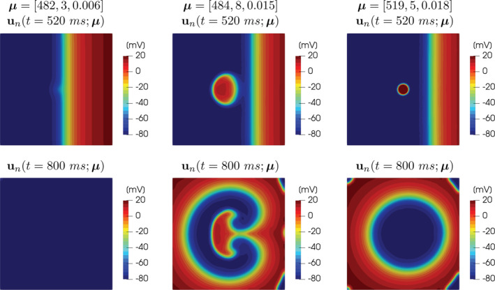
FIGURE 1.

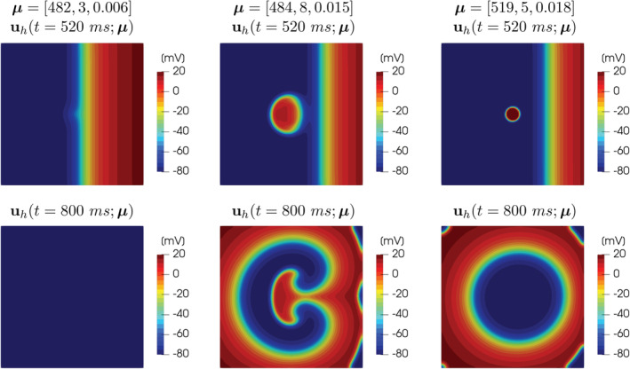
FOM solutions of the monodomain system coupled with the Aliev‐Panfilov ionic model for different values of the parameters, at t = 520 ms and t = 800 ms. The great variability of the solution with respect to the parameters μ ₁, μ ₂, μ ₃ is clearly visible: from left to right, tissue refractoriness, sustained reentry and non‐sustained reentry cases are reported

1. tissue refractoriness: S2 is delivered when the tissue is still in a refractory state and is not yet excitable (see Figure 1, left);

2. sustained reentries: S2 is delivered in the vulnerable window, such that the propagation of the circular depolarization wave is blocked rightward when it encounters refractory tissue, but not leftward where the tissue has already recovered its excitability after the passage of the first wave. This mechanism results in two reentrant circuits around each singularity, forming the so‐called figure of eight (see Figure 1, center);

3. non‐sustained reentry: S2 is delivered after the vulnerability window, such that the propagation of the circular depolarization wave is not blocked rightward, but only slowed down. This mechanism results in a second activation of the tissue, however without producing reentrant circuits (see Figure 1, right).

In order to construct a classifier of this three possible outcomes, we consider as output QoI the deviation between the activation map from a reference value,

$$y\left(\mathit{\mu }\right)=\frac{\parallel \mathit{AT}\left(\mathbf{x};\mathit{\mu }\right)-{\mathit{AT}}_{\mathit{ref}}\left(\mathbf{x}\right){\parallel }_2}{\parallel {\mathit{AT}}_{\mathit{ref}}\left(\mathbf{x}\right){\parallel }_2}.$$

Here AT(x; μ) is the activation time, which provides information about the last recorded time when the electric wavefront has reached a given point of the computational domain. Indeed, given the electric potential $\tilde{u}=\tilde{u}\left(\mathbf{x},\tilde{t};\mathit{\mu }\right)$, the (unipolar) activation map at a point x ∈ Ω is evaluated as the minimum time at which the AP peak reaches x; from a practical standpoint, we can evaluate the activation time as the time at which the time derivative of the transmembrane potential is maximized, that is,

$$\mathit{AT}\left(\mathbf{x};\mathit{\mu }\right)=\arg \underset{\tilde{t}\in \left(T_1,T_2\right)}{\max }\left|\frac{\partial u}{\partial t}\left(\mathbf{x},\tilde{t};\mathit{\mu }\right)\right|,$$

being (T ₁, T ₂) the latest time depolarization‐polarization interval in which the potential exceeded a certain threshold.

In our case, AT _ref is a reference activation map, obtained for μ ₃ = 0.0125, when no S2 stimulus is delivered. By construction, values of the output QoI y(μ) ≈ 0 indicate that the tissue is refractory; instead, reentries are induced when y(μ) > 0. In our numerical tests, we observed that for values of the output close to 2 the reentry was not sustained, while for values of the output larger than 2.5 the reentry was sustained. Figure 2 shows a summary of the considered input–output relationship.

FIGURE 2.

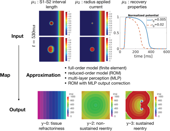
Graphical sketch of the input–output map. Input parameters (top) are related with the time interval between S1 and S2 stimuli (μ ₁), the radius of the circular region in which S2 is applied (), and the tissue recovery properties, modeled by the coefficient ε ₀ affecting the ionic model (μ ₃). The output quantity of interest y(μ) represents the deviation of the activation map from a reference value, evaluated as a scalar index and acts as a classifier: small values of the output are related with tissue refractoriness, intermediate values with non‐sustained reentry, large values with sustained reentry. Being dependent of the transmembrane potential u(μ), the output y(μ) can be evaluated exploiting one of the proposed models: a reduced order model (ROM), an ANN‐based emulator (MLP), a ROM corrected with an ANN‐based emulator for the ROM error (ROM+MLP)

All computational timings shown below are obtained by performing calculations on an Intel(R) Core i7‐8700 K CPU with 64 Gb DDR4 2666 MHz RAM using Matlab(R). The physical coefficients considered for the monodomain (1) and the ionic (2) models are reported in Table 1.

TABLE 1.

Values (taken from Reference 70) of the model physical coefficients employed in the numerical simulations

K	a	c 1	c 2	b	Dii(mm2/ms)
8	0.01	0.2	0.3	0.15	0.2

3.1. Full order model

We introduce on a square domain of size (0, 10) × (0, 10) cm² a structured triangular grid made by 20,000 triangular elements, and N _h = 10, 201 vertices, resulting by choosing a maximum element size equal to h = 1.0 mm and consider over the time interval [0, 1000] ms a time step equal to Δt = 0.5 ms. We build the FOM (3) and (4) through the finite element method, using linear finite elements; a single query to the FOM takes 2 min 25 s to be computed.

In this respect, a comment about mesh resolution is in order. Indeed, we compare the activation times computed for different choices of (h, Δt) = (1.0 mm,0.5 ms), (0.5 mm,0.25 ms), and (0.25 mm,0.125 ms). Results obtained for different choices of the parameters (representative of the different scenarios that will be discussed later) are reported in Figure 3. Differences are almost negligible in terms of activation times among the three different setting, thus motivating the use of a discretization with (h, Δt) = (1.0 mm,0.5 ms) for the case at hand. However, we highlight how this choice could reveal less appropriate when dealing with cardiac electrophysiology on realistic geometries – and, more importantly, when using realistic cell models and tissue anisotropic and inhomogeneous conductivities; here, our focus is on a benchmark problem involving a simple two‐dimensional slab. Another reason motivating our choice is the need to compare the results obtained with the proposed reduced order (or surrogate) models with the ones provided by the FOM. Indeed, the computational cost entailed by a single query to the FOM would increase to 6 min 51 s (resp., 60 min 22 s) when considering (h, Δt) = (0.5 mm,0.25 ms) (resp., (h, Δt) = (0.25 mm,0.125 ms)), thus making the numerical comparisons impracticable.

FIGURE 3.

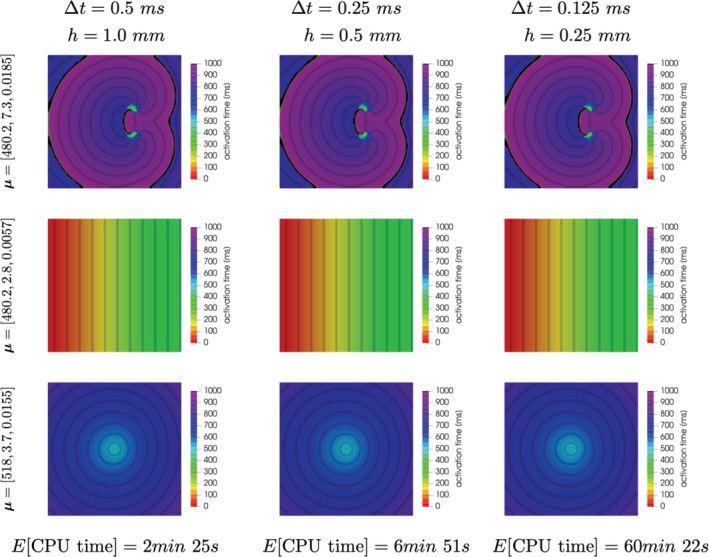
Activation maps computed from the FOM solution for different choices of (h, Δt) = (1.0 mm,0.5 ms), (0.5 mm,0.25 ms), and (0.25 mm,0.125 ms) (from left to right) and different parameter values describing sustained reentry, tissue refractoriness, or non‐sustained reentry (from top to bottom)

3.2. Physics‐based ROMs

We then assess the computational performance and the accuracy of the ROM built by considering the k‐means algorithm for the construction of local ROMs in the state space, according to the strategy proposed in Reference 47. We start from a training sample of 48 parameter vectors selected through Latin hypercube sampling to compute N _c = 6 centroids and the transformation matrices ${\mathbb{V}}_1,\dots ,{\mathbb{V}}_{N_c}$ for the PDE solution on each cluster. With a prescribed POD tolerance of 10⁻², we obtain a maximum (over the N _c clusters) number of basis functions of 205 and a minimum of 51. Then, DEIM is used to approximate the nonlinear term using a training sample of 66 random parameter vectors and exploiting the same local reduced basis structure. In this case, we prescribed a tolerance of 10⁻⁶, resulting in a maximum (over the clusters) number of basis functions of 2585 and a minimum of 950.

Compared to the FOM, the ROM computes a solution to the problem for any new selected parameter instance with a speed‐up of 25 times; see Figure 4 for the comparison between FOM and ROM solutions. The resulting ROM output QoI y _n(μ) approximates the FOM output QoI y _h(μ) with a mean square error of 0.0308 evaluated over a test set formed by 300 random parameter samples.

FIGURE 4.

ROM solutions of the monodomain system coupled with the Aliev‐Panfilov ionic model for different values of the parameters, at t = 520 ms and t = 800 ms

To have a better insight on the ROM accuracy, we report in Figure 5 the singular values of both the solution and the nonlinear term snapshots set, after their partitioning into N _c clusters. The decay of the singular values is directly related with the projection error of the snapshots onto the low‐dimensional subspace spanned by the first singular vectors; this can be seen (up to some constant) as an estimate of the error between the ROM approximation and the FOM solution. Moreover, we report the errors between the ROM and the FOM solutions, obtained on a test set of dimension N _test = 25 sampled from $\mathcal{P}$, for decreasing POD tolerances, in Figure 6, reflecting an increasing accuracy of the ROM for smaller POD tolerances, and showing an almost exponential convergence of the error.

FIGURE 5.

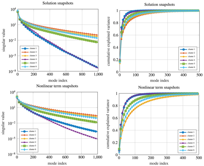
Singular values decay and cumulative expressed variance for the solution (top) and the nonlinear term (bottom) snapshot sets, after their clustering obtained through the k‐means algorithm. The query to extremely accurate ROM might be computationally demanding due to the high number of retained POD modes

FIGURE 6.

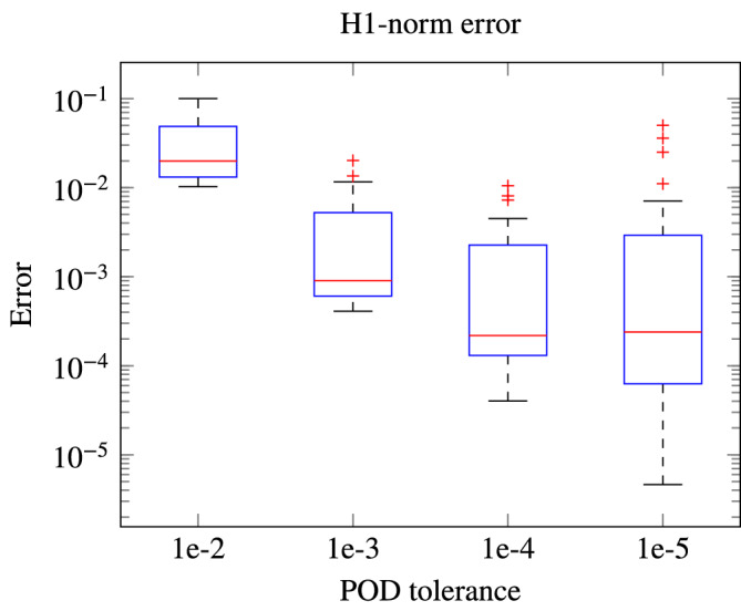
Relative errors on solution obtained with ROMs of increasing accuracy. For decreasing POD tolerances, ROMs of increasing dimensions allow us to obtain decreasing error norms on the solution. The (H ¹(Ω)) computed norm for the solution error sums errors on both the solution and its spatial derivatives. Note that the ROMs with POD tolerances 10⁻⁵ (resp., 10⁻⁴, 10⁻³) are 5 (resp., 4, 1.7) times slower than the ROM with POD tolerance 10⁻²

To correct the ROM output QoI through a NN regression model, we adopt a MLP formed by two hidden layers with 12 nodes each and sigmoids activation functions; the corrected ROM output QoI is denoted by y _n,c(μ). The net is trained using the BFGS quasi‐Newton method to reproduce the FOM output QoI starting from a training set $\mathcal{T}={\left\{\left(\mathit{\mu },y_n\left(\mathit{\mu }\right)\right),y_h\left(\mathit{\mu }\right)\right\}}_{\mathit{\mu }\in {\mathcal{P}}_{\text{train},\mathrm{c}}}$ of $N_{\text{offline},\mathrm{c}}=\mid {\mathcal{P}}_{\text{train},\mathrm{c}}\mid =1700$ output values. In particular, we precompute 2000 output realizations from the FOM and the ROM; the first 1400 realizations are used for the MLP training, 300 are used for the validation and the last 300 for testing (so that N _offline,c = 1400 + 300 = 1700). In this setting the best performance on the validation set is reached at epoch 434 with an MSE of 1.56 ⋅ 10⁻³ and a MSE of 2.7 ⋅ 10⁻³ on the test set (see Figure 7).

FIGURE 7.

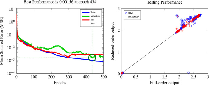
MLP construction of the correction of the ROM output QoI. Left: convergence of the training in terms of MSE over the epochs on the training, validation, and test sets. Right: testing performance of the MLP correction of the ROM output

3.3. Black‐box MLP model

As alternative to the (corrected) ROM output, we also consider the prediction y _MLP(μ) of a NN regression model, built by training a net which emulates the input–output map μ ↦ y _h(μ). Also in this case, we consider a MLP formed by two hidden layers with 12 nodes each and sigmoids activation functions. The training dataset is formed by input–output samples $\mathcal{T}={\left\{\mathit{\mu },y_h\left(\mathit{\mu }\right)\right\}}_{\mathit{\mu }\in {\mathcal{P}}_{\text{train}}}$; also in this case, the training set (including validation points) has cardinality $N_{\text{offline}}=\mid {\mathcal{P}}_{\text{train}}\mid =1700$. The absence of the ROM output QoI as additional input to the net affects the accuracy of the output QoI approximation: the best performance on the validation set is reached at epoch 122 with an MSE of 6.3 ⋅ 10⁻³ and a corresponding MSE of 2.8 ⋅ 10⁻² on the testing set (see Figure 8). Computational costs related to the evaluation of the MLP output QoI are negligible: for each new $\mathit{\mu }\in \mathcal{P}$, the computation of the output requires only a small number of operations, since there are only 12 neurons per layer.

FIGURE 8.

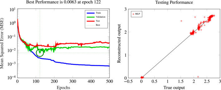
MLP construction of the ANN‐based input–output surrogate. Left: convergence of the training procedure in terms of MSE over the epochs on the training, validation, and test sets. Right: testing performance of the MLP output

However, the computational bottleneck arising when training this MLP model is dataset generation, which requires 1700 FOM queries. Such amount of FOM evaluations is feasible in this setting, but would be out of reach when dealing with patient‐specific 3D simulations with finer meshes and smaller time steps. On the other hand, as the number of training samples decreases, we observe an increase in the MSE error on the test set (see Figure 9) – hence, a MLP surrogate model can be reliable, for the case at hand, only provided it has been trained on a sufficiently large dataset. Indeed, if we consider only N _offline = 100 training samples, the error is an order of magnitude larger than the one given by the same MLP model trained on N _offline = 1700 data. On the other hand, the information provided by a physics‐based ROM helps in improving, by at least one order of magnitude, the accuracy of the black‐box MLP, hence giving the possibility to use also small samples for the MLP training (and, as a consequence, to reduce the cost of the training phase dramatically).

FIGURE 9.

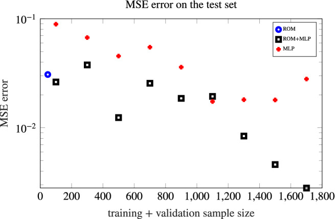
Accuracy of the MLP and ROM+MLP models in terms of mean squared error (MSE) over the test set, plotted as a function of the size N _offline of training+validation sample. The ROM+MLP is more accurate than the MLP (in terms of MSE error), and definitely outperforms the MLP for N _offline > 1000. The MSE error provided by the ROM is also reported

From Figure 9 we also highlight that the ROM+MLP is more accurate than the MLP (in terms of MSE error), and definitely outperforms the MLP for N _offline > 1000. Hence, provided a huge snapshots set from the FOM is available, the ROM+MLP strategy (involving a physics‐based ROM) is preferable with respect to the MLP (which is purely data‐driven), for the same online computational cost. Moreover, keeping the (offline) computational effort comparable, using a MLP to obtain a corrected ROM output, rather than the output itself, is a better option. On the other hand, compared to the ROM, a corrected ROM provides significant improvements only provided the number of FOM solutions used for its training is sufficiently large.

3.4. Sensitivity analysis

We now perform the variance‐based GSA for the case at hand, using the Sobol’ method with N _s = 10⁴, comparing the following options for the input–output map:

• the FOM output QoI μ ↦ y _h(μ);

• ROM, the ROM output QoI μ ↦ y _n(μ);

• MLP (100), the MLP output QoI μ ↦ y _MLP(μ), with N _offline = 100;

• MLP (1700), the MLP output QoI μ ↦ y _MLP(μ), with N _offline = 1700;

• ROM + MLP (100), the corrected ROM output QoI through a MLP model, (μ, y _n(μ)) ↦ y _n,c(μ), with N _offline,c = 100;

• ROM + MLP (1700), the corrected ROM output QoI through a MLP model, (μ, y _n(μ)) ↦ y _n,c(μ), with N _offline,c = 1700.

Regarding the ROM, the corrected ROMs and the MLP outputs, we group these options in two classes, depending on the number of FOM snapshots used to build the corresponding ROM/surrogate model: the ROM, MLP (100) and ROM+MLP(100) are characterized by a small dataset size, while MLP(100) and ROM+MLP (1700) are characterized by a large dataset size. For each option, we report the main effect plots and compute the sensitivity indices defined in (9) and (11).The so‐called main effect plots, showing the output mean (with respect to μ _∼i) as a function of each input μ _i, i = 1,2,3, are useful to visualize, intuitively, if different levels of an input affect the output differently. For the case at hand, main effect plots are reported in Figure 10 considering 10 levels for each input and show that, in general, the output QoI is strongly influenced by changes in the third parameter (modeling the recovery property of the tissue). Moreover, the output is close to 1 only for small values of the third parameter, thus indicating that there are several scenarios of tissue refractoriness. From these results, we can also observe that when the stimulus is released later in the time window spanned by the first parameter (corresponding to high values of μ ₁), it is less likely that the reentry is sustained. All the models allow to observe these main characteristics, except for the MLP (100), which shows remarkable distortions of the curves with respect to the FOM ones (used as reference), hence leading to different conclusions regarding the impact of parameter variations on the tissue response. Instead, the ROM yields only a significant distortion of the third curve (yellow one). However, this error is only slightly reduced by the ROM‐MLP (100), but is almost eliminated by the ROM‐MLP (1700), which is the closest one to the FOM results in terms of accuracy.

FIGURE 10.

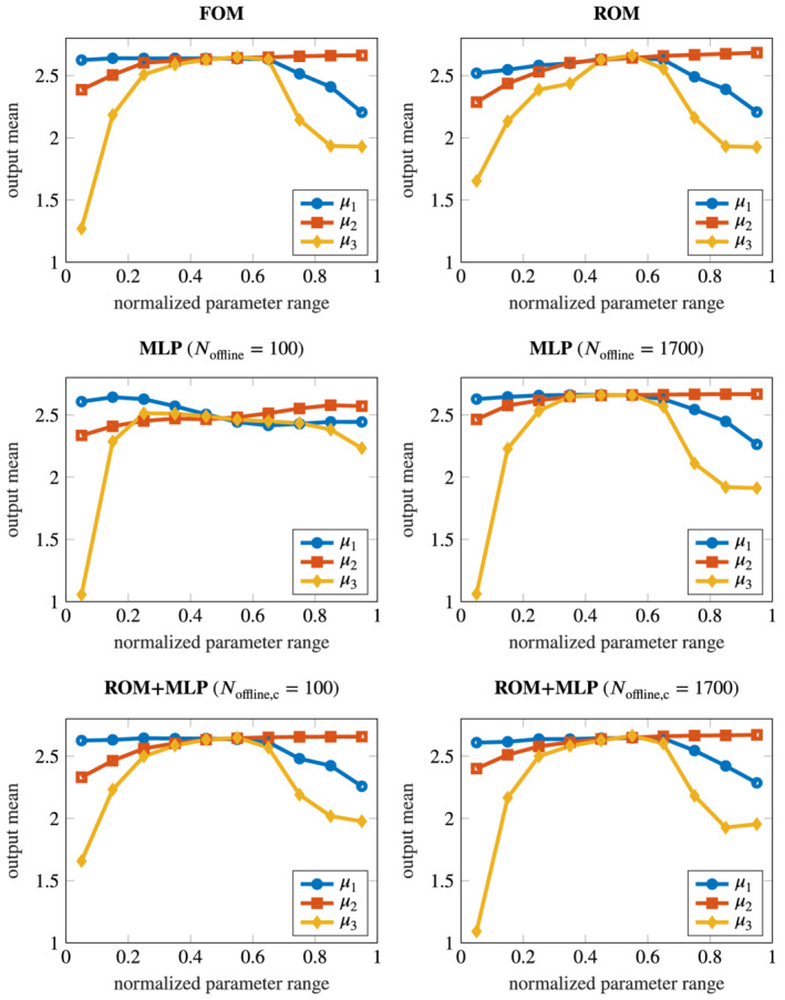
Main effect plots obtained with the six considered models, showing the output mean (with respect to μ _∼i) as a function of each input μ _i, i = 1,2,3. From top to bottom, from left to right: FOM, ROM; MLP (100); MLP (1700); ROM+MLP (100), ROM+MLP (1700). Main effect plots are useful to visualize if different levels of each μ _i affect the output differently

The analysis of the first‐order sensitivity and the total effect indices (see Table 2) shows that:

TABLE 2.

First order sensitivity indices S _i and total effect indices $S_{T_i}$ of the parameters μ _i, i = 1,2,3, on the output computed with the six considered models

	N s	S 1	S 2	S 3	$S_{T_1}$	$S_{T_2}$	$S_{T_3}$
FOM	103	.0209	.0539	.4383	.4305	.2940	.9091
Small dataset size
ROM	103	.0109	.0623	.3649	.4562	.3616	.9012
ROM+MLP (100)	103	.0015	.0575	.4095	.4261	.3284	.9213
MLP (100)	103	.0355	.0737	.5243	.3676	.2936	.9094
Large dataset size
ROM+MLP (1700)	103	.0315	.0663	.4351	.4249	.2939	.9275
MLP (1700)	103	.0213	.0585	.4530	.4185	.2892	.9310

Note: In all cases, Monte Carlo (MC) estimates have been considered according to formulas (12) and (13), in which N _s MC samples have been generated (for a total number of (p + 2)N _s queries to the model.

1. fixing the value of the tissue recovery property does not reduce considerably the output variance (in fact, S ₃ is close to .45, while S ₁ and S ₂ are much smaller than S ₃);

2. the sum of first‐order sensitivity indices S _i is much lower than one, indicating the presence of interactions among parameters;

3. ε ₀ is the most influential among the three parameters, as shown by the computed value of $S_{T_3}$, which is approximatively twice as the value of $S_{T_1}$ or $S_{T_2}$;

4. the sum of the total effect indices $S_{T_i}$ is greater than 1, meaning that the model is nonadditive. ⁵

Note that the approximation error introduced by efficient input–output models impacts with some bias on the resulting indices: for instance, S ₃ is overestimated using the MLP (100) (0.5243 instead of 0.4383), and underestimated using the ROM (0.3649 instead of 0.4383). As remarked for the main effects plots, the corrected ROM‐MLP (1700) is the most accurate one when compared to the FOM (S ₃ = 0.4351). For this specific example, the observed bias on the indices does not lead to different conclusions on the effects of the parameters on the output. However, when a larger number of parameters is involved, biased sensitivity indices might lead to wrong analysis and conclusions about the role of the parameters with respect to the output QoI.

3.5. Forward uncertainty quantification

We now consider uncertainty propagation on the output of interest by using Monte Carlo sampling based on N _mc = 1000 evaluations of the input–output map. In a first test case, we consider six different configurations with uniform distributions, characterized by the following supports:

1. Case 1: {480} × [2.5,8.5] × [0.005,0.02], to describe scenarios with fixed early ectopic impulse;

2. Case 2: {520} × [2.5,8.5] × [0.005,0.02], to describe scenarios with fixed late ectopic impulse;

3. Case 3: [480,520] × {2.5} × [0.005,0.02], to describe scenarios with fixed small radius of the impulse;

4. Case 4: [480,520] × {8.5} × [0.005,0.02], to describe scenarios with fixed large radius of the impulse;

5. Case 5: [480,520] × [2.5,8.5] × {0.005}, to describe scenarios with fixed long APD;

6. Case 6: [480,520] × [2.5,8.5] × {0.02}, to describe scenarios with fixed short APD.

The resulting distributions of the output QoI obtained with the six options for the input–output map previously described are reported in Figures 11 and 12; sample means, sample variances and resulting coefficient of variations are reported in Table 3. We obtain that case (4), involving an impulse with a fixed large radius, is the one yielding to the larger probability of having a sustained reentry. This result is shared by all the considered approximations of the input–output map except for the MLP (100). In this latter case (see Figure 11, bottom‐center plot) we obtain an output distribution less skewed and with smaller mean. In general, the effect of the approximation error impacts on the output QoI distributions: indeed, using less accurate models might result in distributions showing larger skewness or variances, and in means affected by some discrepancies compared to the results obtained with the FOM.

FIGURE 11.

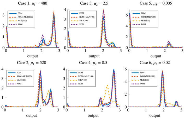
Output QoI distributions resulting from forward propagation obtained with the ROM, the ROM+MLP (100) and the MLP (100) models (hence, in presence of a small dataset size), compared with the FOM output QoI distribution

FIGURE 12.

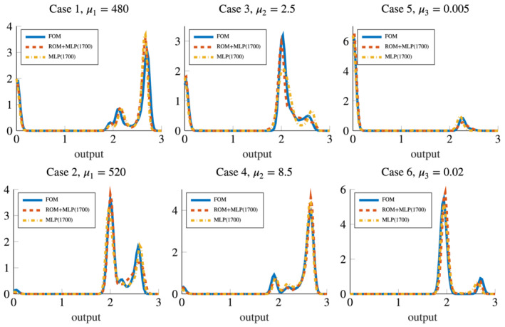
Output QoI distributions resulting from forward propagation obtained with the ROM+MLP (1700) and the MLP (1700) models (hence, in presence of a large dataset size), compared with the FOM output QoI distribution

TABLE 3.

Uncertainty propagation: sample mean, standard deviation and coefficient of variation of the output QoI computed with the different models, in cases 1, …, 6

		Case 1	Case 2	Case 3	Case 4	Case 5	Case 6
		μ 1 = 480	μ 1 = 520	μ 2 = 2.5	μ 2 = 8.5	μ 3 = 0.005	μ 3 = 0.02
FOM	Mean	1.8581	2.1607	1.6635	2.3927	.3588	2.0281
	Standard deviation	1.1238	.3933	.8983	.5810	.8180	.2521
	Coeff. of variation	.6048	.1820	.54	.2428	2.2798	.1243
Small dataset size
ROM	Mean	1.8580	2.1593	1.6273	2.4289	.4179	2.0207
	Standard deviation	1.0830	.3455	.8482	.5598	.8553	.2550
	Coeff. of variation	.5829	.16	.5212	.2305	2.0466	.1261
ROM+MLP (100)	Mean	1.8851	2.1305	1.6088	2.4229	.4041	2.0510
	Standard deviation	1.1075	.3526	.8705	.4873	.8444	.2497
	Coeff. of variation	.5875	.1655	.5411	.2011	2.0896	.1214
MLP (100)	Mean	1.9099	2.1297	1.6234	2.2949	.554	2.129
	Standard deviation	1.1768	.3680	.8376	.4743	.8478	.3195
	Coeff. of variation	.6161	.1727	.5159	.2067	1.5303	.15
Large dataset size
ROM+MLP (1700)	Mean	1.9336	2.2045	1.6141	2.4196	.3265	2.0376
	Standard deviation	1.0773	.3367	.9246	.5595	.7778	.2188
	Coeff. of variation	.5571	.1527	.5728	.2312	2.3822	.1074
MLP (1700)	Mean	1.8598	2.1848	1.6489	2.4247	.3693	2.0288
	Standard deviation	1.1170	.3599	.9342	.4976	.8125	.2154
	Coeff. of variation	.6006	.1647	.5665	.2052	2.2001	.1062

In a second test case, we consider simultaneous variations of all parameters, and restrict the support of the input parameter (uniform) distribution, after normalizing each parameter to the [0, 1] range, for the sake of variance shrinking, thus aiming at reducing the effects of sampling variation. Denoting by

$${\tilde{\mu }}_i=\frac{{\mu }_i-{\mu }_i^{\min }}{{\mu }_i^{\max }-{\mu }_i^{\min }}\in \left[0,1\right],i=1,\dots ,3,$$

we consider four different options, by sampling uniformly in the set

$${\mathrm{\Xi }}_{\alpha }=\left\{\left(\alpha ,1-\alpha \right){\tilde{\mu }}_i,i=1,\dots ,3\right\}\subset {\mathrm{ℝ}}^3$$

with α = 0.1,0.2,0.3,0.4, respectively. For each input distribution, we compute the output mean and standard deviation (see Table 4) using all the approximations of the input–output map previously described. The most significant bias in the mean is observed when using the MLP output QoI trained with only N _offline = 100 input–output observations, and when the input distribution support decreases. Regarding the variance, we observe that the largest discrepancies arise from the use of the MLP output QoI, with a recurrent underestimation of the output variance when the MLP is trained on the smallest dataset. On the other hand, a slightly greater variance is obtained when using the ROM output QoI, compared to the FOM case: the cause of the mild variance increase might be related to the propagation of the ROM approximation error in the output. Once again, correcting the ROM output QoI with a MLP model seems the best option, yielding the closest result to what we would obtain if we relied on the FOM output QoI to perform forward uncertainty propagation.

TABLE 4.

Uncertainty propagation: sample mean, standard deviation and coefficient of variation of the output QoI computed with the different models, in cases 1, …, 6 (variance shrinking scenario)

		U([0.1,0.9]3)	U([0.2,0.8]3)	U([0.3,0.7]3)	U([0.4,0.6]3)
FOM	Mean	2.2877	2.4545	2.5612	2.6369
	Standard deviation	.5701	.2875	.1943	.0161
	Coeff. of variation	.2492	.1171	.0759	.0061
Small dataset size
ROM	Mean	2.2658	2.4031	2.5177	2.6365
	Standard deviation	.5277	.2935	.2218	.0461
	Coeff. of variation	.2329	.1221	.0881	.0175
ROM+MLP (100)	Mean	2.2941	2.4517	2.5554	2.6382
	Standard deviation	.528	.2617	.1839	.0221
	Coeff. of variation	.2301	.1067	.072	.0084
MLP (100)	Mean	2.2911	2.4542	2.4916	2.4764
	Standard deviation	.5163	.1965	.0737	.0421
	Coeff. of variation	.2253	.0801	.0296	.017
Large dataset size
ROM+MLP (1700)	Mean	2.2880	2.4542	2.5642	2.6445
	Standard deviation	.5669	.2890	.2004	.0245
	Coeff. of variation	.2478	.1178	.0781	.0093
MLP (1700)	Mean	2.2906	2.4579	2.5725	2.6586
	Standard deviation	.5592	.2912	.2027	.0106
	Coeff. of variation	.2441	.1184	.0788	.004

4. DISCUSSION

4.1. Computational efficiency

The numerical results of the previous section show that, whenever available, a physics‐driven reduced order model approximating the primal variables of the problem can have a remarkable impact on the accuracy of an ANN‐based model, when used for the sake of sensitivity analysis and forward uncertainty quantification.

Regarding the online computational costs, the ROM provides a speedup of about 25 times compared to the FOM; hence, sensitivity analysis can be performed in a CPU time of 8.3 h – rather than 208 h if relying on the FOM – while forward UQ only requires a CPU time of 1.5 h, rather than 83 h. The same analyses performed with the MLP models are even more faster, requiring their online evaluation less than 1 s. Similarly, the online CPU time required by the ROM+MLP models is almost equal to the one employed by the ROM. See Figure 13 for the comparison between online and offline costs entailed by a single query to the proposed models.

FIGURE 13.

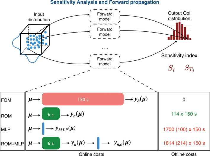
Comparison between online and offline costs entailed by the proposed models. Performing forward UQ requires N _mc evaluations of the output QoI, while GSA requires (p + 2)N _s evaluations of the output QoI. For the case at hand, N _mc = 1000, p = 3 and N _s = 10⁴

Regarding instead the offline computational costs, we remark that the proposed ROM only requires 114 evaluations of the FOM for the sake of POD basis construction, resulting in a CPU time of about 5 h. MLP and ROM+MLP models require instead many more FOM evaluations, with a CPU time of about 4 h for MLP (100), 9 h for ROM+MLP (100), 70 h for MLP (1700), 76 h for ROM+MLP (1700).

From the computed results, we have shown that ROM+MLP models are definitely better than MLP models, with a remarkable gain in terms of accuracy, and one order of magnitude more accurate than the ROM model. Increasing the ROM accuracy is of course possible by considering a large number n of basis functions. However, this option would increase the online computational costs, yielding to a potentially smaller speedup compared with the use of a FOM. We underline that the tradeoff between accuracy and efficiency is problem‐dependent, and what really makes the difference is the computational speedup between the ROM and the FOM, rather than the relationship between the ROM dimension and the corresponding online time. Otherwise said, for the case at hand, the speedup between the FOM and the ROM is about 25, and a factor 5 extra computational cost for the ROM (that would ensure a factor 10³ better error) would drop the speedup to only 5, thus making the overall cost of the analysis extremely large.

On the other hand, the online evaluation of an ANN‐based model for the error is almost inexpensive. Indeed, we can obtain the same accuracy of a higher dimensional ROM (which is, however, computationally demanding online, due to the high number of retained POD modes) by using a corrected ROM+MLP model built with a small ROM dimension, provided a large solution dataset is available. On the other hand, provided the same number of FOM problems is solved offline, an approach involving a ROM like the ROM+MLP model, is definitely more convenient than a purely data‐driven model, like the MLP, in terms or resulting accuracy. For these reasons, we propose to rely on a sufficiently accurate ROM with preferably smaller dimension, and to correct its outcome with an inexpensive ANN‐based model, rather than increasing the ROM dimension too much.

We also highlight that the purpose of our work is to set, analyze and apply physics‐based and/or data‐driven techniques in order to enable UQ in cardiac electrophysiology; the other two pillars of VVUQ analysis – verification and validation – do not fit among the goals of this work. The former task, verification, establishes how accurately a computer code solves the equations of a mathematical model; the latter, validation, determines how well a mathematical model represents the real world phenomena it is intended to predict. Nevertheless, results reported in Section 3 provide some insights into: the FOM calculation verification, since spatio‐temporal discretization convergence has been performed on the FOM solution (Section 3.1); the ROM calculation verification, having assessed the ROM convergence with respect to the number of basis functions for both the primal variable and the output quantity of interest (Section 3.2); the validation of the proposed framework against the results obtained with the FOM, here treated as truth high‐fidelity solution (Sections 3.4 and 3.5).

4.2. Further extension to more realistic scenarios

The most common atrial arrhythmias, also called supraventricular arrhythmias, are atrial fibrillation and atrial flutter. In the former, the atria are activated with a disorganized pattern, while in the latter the activation follows a regular, but self‐sustained and accelerated, pattern. The ectopic beats are considered as a common trigger of atrial arrhythmias. In order to be effective, the ectopic foci must find a combination of factors, mainly related to the electrophysiological characteristics of the tissue, such as conduction properties and refractory period duration. ⁷¹ As shown in the simplified case we considered, impulses persist to re‐excite the tissue autonomously only provided that suitable conditions are verified – that is, whenever there is an appropriate substrate for re‐entry. The numerical results confirm that the duration of the refractory period (controlled in our case by the physical coefficient of the ionic equation ɛ₀) is a key factor for the sustainment of the reentry: the longer the refractory periods, the less likely is the re‐entry sustainment, due to the head‐tail interaction of the impulse in the reentry circuit. This kind of interaction can be also modified by considering different dimensions of the isthmus of the figure of eight reentry, which is in our examples determined by the dimension of the ectopic foci.

Our study shows how to extract meaningful indices related to sustainability of reentry in a context of uncertain inputs. The proposed framework, merging physics‐based reduced‐order models and artificial neural networks, could enhance the quantitative description of a range of possible (physiological and pathological) phenomena, possibly dealing with more complex scenarios, where also anisotropy in electric signal conduction and specific ionic concentration variations are taken into account. We have realized a proof of concept showing a possible way to translate our results into a more realistic scenario, where numerical simulations have been run on a left atrium geometry, see Figure 14. As realistic geometry, we use the Zygote solid 3D heart model, ⁷² a complete heart geometry reconstructed from high‐resolution CT‐scans representing an average healthy heart. As shown in Reference 73, atrial ectopic beats can be found mostly in the pulmonary veins (with the highest incidence in the left superior pulmonary vein); a possible strategy to avoid that arrhythmias are induced consists of the electrical isolation of the veins with radio‐frequency ablation. ⁷³ , ⁷⁴ Hence, we consider the case where the ectopic beat is located on the left superior pulmonary veins, and explore different scenarios on the basis of the numerical results obtained in the previous, two‐dimensional case.

FIGURE 14.

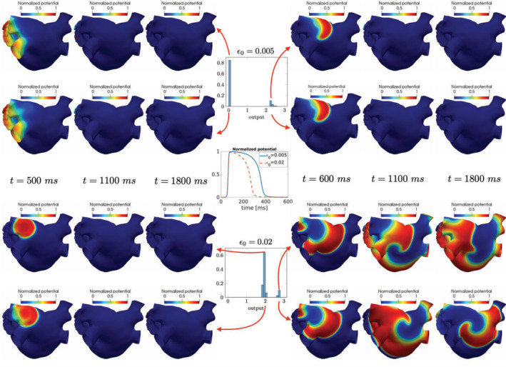
Electric potential computed on a 3D template left atrium geometry for different parameter values. The input–output setting described for the two‐dimensional case can represent a first step towards the classification of different conditions also on more complex configurations

In Figure 14 we have reported the (normalized) electric potential computed on a template left atrium geometry, over time, by fixing a value of μ ₃ = ε ₀ and thus considering two different scenarios (ε ₀ = 0.005 and ε ₀ = 0.02, respectively) regarding the tissue recovery property. Since in these two cases the values of the output QoI are clustered around two opposite values (see, e.g., the results obtained for Cases 5 and 6 in Figures 11 and 12), we randomly sample from the distributions of μ ₁ and μ ₂ and compute the corresponding electric potential over time. As highlighted in Figure 14, the conclusions reached for the two‐dimensional case prove to be useful to classify possible scenarios occurring in a left atrium geometry. Also in this case, we indeed obtain a sustained reentry provided that ε ₀ = 0.02, and the output QoI takes larger values. In this respect, the analysis performed on the simplified two‐dimensional test case might be helpful in view of a systematic investigation of the effect of physical parameters (related with both the stimulation protocol and the ionic activity) on complex patterns including spiral waves reentry.

4.3. Comparison with other existing approaches

The analysis we carried out is the first attempt of integrating a physics‐based surrogate model built through rigorous reduced‐order modeling techniques such as the POD‐Galerkin method, and an ANN regression model properly accounting for the approximation error between the FOM and the ROM.

So far, only few papers have addressed a systematic uncertainty quantification (UQ) and propagation in cardiac electrophysiology models, despite the very rapid growth of cardiac modeling and the need to deal with multiple scenarios, towards model personalization. For instance, the role of infarct scar dimensions, border zone repolarization properties and anisotropy in the origin and maintenance of cardiac reentry has been considered in Reference 75; the evaluation of cardiac mechanical markers (such as longitudinal and circumferential strains) to estimate the electrical activation times has been addressed in Reference 76. See, for example References 2, 77, for a review of the possible sources of uncertainty in these models at different spatial scales.

A systematic uncertainty quantification and sensitivity analysis in cardiac electrophysiology models must necessarily rely on surrogate models, because of the computational bottlenecks entailed by the need to query the input–output map repeatedly. Usual paradigms for the construction of surrogate models have relied on either lower‐fidelity models or emulators:

• regarding the use of lower‐fidelity models, forward UQ has been performed on a simplified Eikonal model in Reference 78, where statistics of the activation map (e.g., activation time at a specific point of the left ventricle) have been computed given the uncertainty associated with the conductivity tensor modeling the fiber orientation, exploiting Bayesian multi‐fidelity methods combining the Eikonal model and a physics‐based simplification of this latter. Although possible – see, for example, ⁷⁹ , ⁸⁰ , ⁸¹ – the use of the Eikonal model to describe re‐entrant activity is not straightforward, if one aims at taking properly into account both activation and depolarization phases. A simplified one‐dimensional surrogate model providing a cable representation of a three‐dimensional transmural section across the ventricular wall has been considered in Reference 38, where a multi‐fidelity Gaussian process (GP) regression has been exploited to assess the effect of ion channel blocks on the QT interval;

• several papers have focused on the use of emulators such as GP regression or generalized polynomial chaos expansions (PC) of the input–output map. For instance, the forward UQ problem of propagating the uncertainty in maximal ion channel conductances to suitable outputs of interest, such as the action potential duration, has been addressed in Reference 3 by means of a Monte Carlo approach exploiting GP emulators. Similar techniques have been used in Reference 5 to quantify the effect of uncertainty on input parameters like fiber rotation angle, ischemic depth, blood conductivity and six bidomain conductivities on outputs characterizing the epicardial potential distribution. A GP surrogate of the exact posterior probability density function has been exploited in Reference 6 for the sake of parameter estimation and model personalization, where the estimation of local tissue excitability in a 3D cardiac electrophysiological model has been performed using input data from simulated 120‐lead electrocardiographic (ECG) data. See also, for example, Reference 82 for model parameter inference based on GP emulation on whole‐heart mechanics, Reference 83 for interpolation of uncertain local activation times on human atrial manifolds and References 84, 85 for the analysis of the effect of wall thickness uncertainties on left ventricle mechanics.

Our technique represents a promising trade‐off between the use of lower‐fidelity models and emulators. Indeed, the ANN regression model can be seen as an emulator, applied to the discrepancy between the FOM and the ROM; this latter might be seen as a lower‐fidelity model, however keeping into account physical complexity (yet featuring a lower computational cost) being built through a projection‐based approach.

Regarding sensitivity analysis, very often elementary effects or one‐at‐a‐time approaches have been preferred to global (e.g., variance‐based) methods when dealing with cardiac electrophysiology (and, more generally speaking, cardiac modeling). For instance, one‐at‐a‐time approaches have been considered in Reference 86, addressing the sensitivity of mechanical biomarkers – like the ejection fraction, the longitudinal fractional shortening, or the wall thickening – to key model parameters (such as, e.g., the end‐diastolic pressure, Windkessel model parameters, active tension, angle of fiber distribution). The parameter uncertainty on two electro‐mechanics coupled models for the excitation‐contraction of the cardiac tissue has been addressed by the authors in Reference 87, evaluating the impact of variability in key maximal conductances on action potential duration and ionic concentrations using generalized PC expansions and the elementary effects method. Sensitivity analysis and parameter screening have been performed in Reference 88 to quantify the sensitivity of left ventricular activation and the electrocardiogram to variation of parameters included in a bidomain system coupled with a Ten Tusscher‐Panfilov model, using local sensitivity analysis techniques. In all these cases, strong interactions among input parameters on the model response cannot be evaluated; indeed, global techniques involving simultaneous changes in model parameters usually provide more detailed information about possible synergistic effects on the output QoI. Moreover, for the sake of computational efficiency, global sensitivity analysis has been often applied to one‐dimensional cardiac cell models, in order to quantify, for example, the impact of (conductance and kinetic) model parameters on threshold, maximum upstroke velocity, time of maximum upstroke velocity, action potential amplitude and duration; see, for example References 4, 38.

Sensitivity analysis through the evaluation of Sobol indices has been performed in Reference 89 on output QoIs such as the inner cavity volume, apex lengthening, wall thickness and volume by considering material parameters that characterize the global myocardial stiffness and the local muscle fiber orientation, however relying on PC expansions and quasi Monte Carlo sampling techniques. A similar analysis, aiming at quantifying the importance of regional wall thickness, fiber orientation, passive material parameters, active stress and the circulatory model in cardiac mechanics, has been addressed in, ⁹⁰ where surrogate models have been again generated through PC expansions. However, this approach might suffer from two limitations, namely (i) the assumption that the output is a smooth function of the input parameters, and (ii) the need of constructing an emulator for each output QoI of interest. Regarding instead the number of parameters that can be taken into account, both the proposed approach and data‐driven emulators such as PC expansions might suffer from this curse of dimensionality. However, as soon as the dependence of the primal variable on the (possibly, many) input parameters is smooth, a projection‐based ROM might require less training data to reach the same degree of accuracy of a PC expansion, hence resulting, overall, more efficient from a computational standpoint.

In this respect, the proposed methodology allows us to perform global sensitivity analysis by keeping computational costs limited. Furthermore, exploiting physics‐based ROMs to approximate the state variables (rather than the input–output map itself) allows us, in principle, to perform sensitivity analysis and UQ on several output QoIs, still relying on the same ROM. An additional training of the ROM must instead be performed as soon as (i) the accuracy on the output QoI is found to be inadequate when dealing with UQ, or (ii) larger parameter variations must be considered. This is, in our opinion, a possible limitation of the proposed approach, which represents, however, a major advancement compared to purely data‐driven emulator because of the possibility of controlling the ROM error, and the chance of constructing a physics‐driven, low‐dimensional approximation of the whole solution field. This facts indeed paves a new way regarding the possibility to perform sensitivity analysis and forward UQ involving more complex (e.g., space and/or time dependent) output quantities of interest in cardiac electrophysiology.

Finally, combining ROMs and ANN regression models enable us to consider output QoIs of arbitrary complexity, which can be inexpensively evaluated once the ROM has been solved for any parameter instance, thus providing very good accuracy despite the regularity of the input–output map. Of course, more advanced neural network architectures could outperform the proposed local ROM (enriched with the ANN‐based error model), or the considered ANN‐based input/output model. However, we highlight how in some cases being able to approximating (efficiently) the physics of the problem – rather than only the input–output map – might compensate a lack of data (often occurring in biomedical applications, and limiting the accuracy of surrogate models). Hence, the better the accuracy of the surrogate and/or reduced‐order models in emulating the physical behavior efficiently, and the less the amount of training data (e.g., requiring the repeated solution of a FOM), the more feasible the sensitivity and forward UQ analyses.

5. CONCLUSIONS

In this paper we have proposed new efficient computational strategies to perform forward uncertainty quantification in parametrized problems arising in cardiac electrophysiology. We have addressed both a variance‐based sensitivity analysis for the selection of the most relevant input parameters, and uncertainty propagation to investigate the impact of intra‐subject variability on outputs related to the cardiac action potential. We have taken advantage of reduced‐order models built through the reduced basis method to enable both uncertainty propagation and sensitivity analysis. The ROM has been finally equipped with artificial neural networks to provide accurate approximation of the output.

Compared to a purely data‐driven approach consisting of ANN‐based models emulating the input–output relationship, the proposed approach provides better results in terms of both accuracy and offline costs. Indeed, numerical results obtained on a two‐dimensional benchmark yielding to a variety of different tissue activation patterns, ranging from tissue refractoriness to sustained reentry waves, have shown that the proposed physics‐based reduction framework based on N _offline = 100 training samples is accurate as the black‐box surrogate ANN‐based models with N _offline = 1700, but with much lower offline costs. The MLP model provides the best online efficiency, but its accuracy and offline costs are highly influenced by the dimensions of the training and validation datasets. Finally, the corrected ROM output QoI through a MLP model with N _offline = 1700 is the most accurate method with respect to the computationally expensive full‐order strategy, and is also able to provide a 25× speedup.

Thanks to a suitable integration of physics‐based ROMs and data‐driven machine learning techniques, the framework proposed in this work can potentially lead to substantial advancements regarding both uncertainty quantification and large‐scale computations related with cardiac electrophysiology.

Pagani S, Manzoni A. Enabling forward uncertainty quantification and sensitivity analysis in cardiac electrophysiology by reduced order modeling and machine learning. Int J Numer Meth Biomed Engng. 2021;37:e3450. 10.1002/cnm.3450

REFERENCES

- 1. Quarteroni A, Manzoni A, Vergara C, Dede L. Mathematical Modelling of the Human Cardiovascular System: Data, Numerical Approximation, Clinical Applications. Cambridge, England: Cambridge University Press; 2019. [Google Scholar]
- 2. Mirams GR, Pathmanathan P, Gray RA, Challenor P, Clayton RH. Uncertainty and variability in computational and mathematical models of cardiac physiology. J Physiol. 2016;594(23):6833‐6847. [DOI] [PMC free article] [PubMed] [Google Scholar]
- 3. Johnstone RH, Chang ET, Bardenet R, et al. Uncertainty and variability in models of the cardiac action potential: can we build trustworthy models? J Mol Cell Cardiol. 2016;96:49‐62. [DOI] [PMC free article] [PubMed] [Google Scholar]
- 4. Pathmanathan P, Cordeiro JM, Gray RA. Comprehensive uncertainty quantification and sensitivity analysis for cardiac action potential models. Frontiers in Physiology. 2019;10:721. 10.3389/fphys.2019.00721. [DOI] [PMC free article] [PubMed] [Google Scholar]
- 5. Johnston BM, Coveney S, Chang ETY, Johnston PR, Clayton RH. Quantifying the effect of uncertainty in input parameters in a simplified bidomain model of partial thickness ischaemia. Med Biol Eng Comput. 2018;56(5):761‐780. [DOI] [PMC free article] [PubMed] [Google Scholar]
- 6. Dhamala J, Arevalo HJ, Sapp J, et al. Quantifying the uncertainty in model parameters using Gaussian process‐based Markov chain Monte Carlo in cardiac electrophysiology. Med Image Anal. 2018;48:43‐57. [DOI] [PMC free article] [PubMed] [Google Scholar]
- 7. Niederer SA, Aboelkassem Y, Cantwell CD, et al. Creation and application of virtual patient cohorts of heart models. Philos Trans R Soc A. 2020;378(2173):20190558. [DOI] [PMC free article] [PubMed] [Google Scholar]
- 8. Colli Franzone P, Pavarino LF, Scacchi S. Mathematical Cardiac Electrophysiology. Cham, Switzerland: Springer; 2014. [Google Scholar]
- 9. Sundnes J, Lines GT, Cai X, Nielsen BF, Mardal K‐A, Tveito A. Computing the Electrical Activity in the Heart. Monographs in Computational Science and Engineering 1. Berlin Heidelberg: Springer‐Verlag; 2007. [Google Scholar]
- 10. Clayton RH, Bernus O, Cherry EM, et al. Models of cardiac tissue electrophysiology: progress, challenges and open questions. Prog Biophys Mol Biol. 2011;104(1):22‐48. [DOI] [PubMed] [Google Scholar]
- 11. Dössel O, Krueger MW, Weber FM, Wilhelms M, Seemann G. Computational modeling of the human atrial anatomy and electrophysiology. Med Biol Eng Comput. 2012;50(8):773‐799. [DOI] [PubMed] [Google Scholar]
- 12. Lopez‐Perez A, Sebastian R, Ferrero JM. Three‐dimensional cardiac computational modelling: methods, features and applications. Biomed Eng Online. 2015;14(1):35. [DOI] [PMC free article] [PubMed] [Google Scholar]
- 13. Robert C, Casella G. Monte Carlo Statistical Methods. New York: Springer‐Verlag; 2013. [Google Scholar]
- 14. Pflüger D, Peherstorfer B, Bungartz H‐J. Spatially adaptive sparse grids for high‐dimensional data‐driven problems. J Complexity. 2010;26(5):508‐522. [Google Scholar]
- 15. Gerstner T, Griebel M. Numerical integration using sparse grids. Numer Algor. 1998;18(3–4):209‐232. [Google Scholar]
- 16. Perkó Z, Gilli L, Lathouwers D, Kloosterman JL. Grid and basis adaptive polynomial chaos techniques for sensitivity and uncertainty analysis. J Comput Phys. 2014;260:54‐84. [Google Scholar]
- 17. Biehler J, Gee MW, Wall WA. Towards efficient uncertainty quantification in complex and large scale biomechanical problems based on a Bayesian multi fidelity scheme. Biomech Model Mechanobiol. 2015;14(3):489‐451. [DOI] [PubMed] [Google Scholar]
- 18. Giles MB. Multilevel Monte Carlo path simulation. Oper Res. 2008;56(3):607‐617. [Google Scholar]
- 19. Nobile F, Tesei F. A multi level Monte Carlo method with control variate for elliptic PDEs with log‐normal coefficients. Stoch Partial Differ. 2015;3(3):398‐444. [Google Scholar]
- 20. Sudret B. Global sensitivity analysis using polynomial chaos expansions. Reliab Eng Syst Safe. 2008;93(7):964‐979. [Google Scholar]
- 21. Nobile F, Tempone R, Webster CG. A sparse grid stochastic collocation method for partial differential equations with random input data. SIAM J Numer Anal. 2008;46(5):2309‐2345. [Google Scholar]
- 22. Gunzburger MD, Webster CG, Zhang G. Stochastic finite element methods for partial differential equations with random input data. Acta Numer. 2014;23:521‐650. [Google Scholar]
- 23. Haykin S. Neural Networks and Learning Machines. 3rd ed. Upper Saddle River, NJ: Pearson Prentice Hall; 2009. [Google Scholar]
- 24. Crestaux T, Le Maitre O, Martinez J‐M. Polynomial chaos expansion for sensitivity analysis. Reliab Eng Syst Safe. 2009;94(7):1161‐1172. [Google Scholar]
- 25. Rasmussen CE, Williams CKI. Gaussian Processes for Machine Learning. Cambridge, MA: the MIT Press; 2006. https://www.GaussianProcess.org/gpml. [Google Scholar]
- 26. Neic A, Campos FO, Prassl AJ, et al. Efficient computation of electrograms and ECGs in human whole heart simulations using a reaction‐eikonal model. J Comput Phys. 2017;346:191‐211. [DOI] [PMC free article] [PubMed] [Google Scholar]
- 27. Jacquemet V. An Eikonal approach for the initiation of reentrant cardiac propagation in reaction–diffusion models. IEEE Trans Biomed Eng. 2010;57(9):2090‐2098. [DOI] [PubMed] [Google Scholar]
- 28. Fenton FH, Cherry EM, Hastings HM, Evans SJ. Multiple mechanisms of spiral wave breakup in a model of cardiac electrical activity. Chaos. 2002;12(3):852‐892. [DOI] [PubMed] [Google Scholar]
- 29. Colli Franzone P, Pavarino LF, Taccardi B. Simulating patterns of excitation, repolarization and action potential duration with cardiac bidomain and monodomain models. Math Biosci. 2005;197(1):35‐66. [DOI] [PubMed] [Google Scholar]
- 30. Nash MP, Panfilov AV. Electromechanical model of excitable tissue to study reentrant cardiac arrhythmias. Prog Biophys Mol Biol. 2004;85(2):501‐522. [DOI] [PubMed] [Google Scholar]
- 31. Qu Z, Xie F, Garfinkel A, Weiss JN. Origins of spiral wave meander and breakup in a two‐dimensional cardiac tissue model. Ann Biomed Eng. 2000;28(7):755‐771. [DOI] [PubMed] [Google Scholar]
- 32. Ten Tusscher K, Panfilov AV. Alternans and spiral breakup in a human ventricular tissue model. Am J Physiol Heart Circ Physiol. 2006;291(3):1088‐1100. [DOI] [PubMed] [Google Scholar]
- 33. Arevalo HJ, Vadakkumpadan F, Guallar E, et al. Arrhythmia risk stratification of patients after myocardial infarction using personalized heart models. Nat Commun. 2016;7:11437. [DOI] [PMC free article] [PubMed] [Google Scholar]
- 34. Hill YR, Child N, Hanson B, et al. Investigating a novel activation‐repolarisation time metric to predict localised vulnerability to reentry using computational modelling. PloS One. 2016;11(3):e0149342. [DOI] [PMC free article] [PubMed] [Google Scholar]
- 35. Relan J, Chinchapatnam P, Sermesant M, et al. Coupled personalization of cardiac electrophysiology models for prediction of ischaemic ventricular tachycardia. Interface Focus. 2011;1(3):396‐407. [DOI] [PMC free article] [PubMed] [Google Scholar]
- 36. Prakosa A, Arevalo HJ, Deng D, et al. Personalized virtual‐heart technology for guiding the ablation of infarct‐related ventricular tachycardia. Nat Biomed Eng. 2018;2:732‐740. [DOI] [PMC free article] [PubMed] [Google Scholar]
- 37. Corrado C, Razeghi O, Roney C, et al. Quantifying atrial anatomy uncertainty from clinical data and its impact on electro‐physiology simulation predictions. Med Image Anal. 2020;61:101626. [DOI] [PubMed] [Google Scholar]
- 38. Costabal FS, Matsuno K, Yao J, Perdikaris P, Kuhl E. Machine learning in drug development: characterizing the effect of 30 drugs on the QT interval using Gaussian process regression, sensitivity analysis, and uncertainty quantification. Comput Methods Appl Mech Eng. 2019;348:313‐333. [DOI] [PMC free article] [PubMed] [Google Scholar]
- 39. Quarteroni A, Manzoni A, Vergara C. The cardiovascular system: mathematical modeling, numerical algorithms, clinical applications. Acta Numer. 2017;26:365‐590. [Google Scholar]
- 40. Aliev RR, Panfilov AV. A simple two‐variable model of cardiac excitation. Chaos Solit Fract. 1996;7(3):293‐301. [Google Scholar]
- 41. Colli FP, Pavarino LF. A parallel solver for reaction–diffusion systems in computational electrocardiology. Math Models Methods Appl Sci. 2004;14(06):883‐911. [Google Scholar]
- 42. Plank G, Liebmann RW, Vigmond EJ, Haase G. Algebraic multigrid preconditioner for the cardiac bidomain model. IEEE Trans Biomed Eng. 2007;54(4):585‐596. [DOI] [PMC free article] [PubMed] [Google Scholar]
- 43. Goktepe S, Kuhl E. Computational modeling of cardiac electrophysiology: a novel finite element approach. Int J Numer Methods Eng. 2009;79(2):156‐178. [Google Scholar]
- 44. Chaturantabut S, Sorensen DC. Nonlinear model reduction via discrete empirical interpolation. SIAM J Sci Comp. 2010;32(5):2737‐2764. [Google Scholar]
- 45. Negri F, Manzoni A, Amsallem D. Efficient model reduction of parametrized systems by matrix discrete empirical interpolation. J Comput Phys. 2015;303:431‐454. [Google Scholar]
- 46. Quarteroni A, Manzoni A, Negri F. Reduced Basis Methods for Partial Differential Equations. An Introduction. Switzerland: Springer International Publishing; 2016. [Google Scholar]
- 47. Pagani S, Manzoni A, Quarteroni A. Numerical approximation of parametrized problems in cardiac electrophysiology by a local reduced basis method. Comput Methods Appl Mech Eng. 2018;340:530‐558. [Google Scholar]
- 48. Barrault M, Maday Y, Nguyen NC, Patera AT. An empirical interpolation method: application to efficient reduced‐basis discretization of partial differential equations. C R Acad Sci. 2004;339(9):667‐672. [Google Scholar]
- 49. Maday Y, Nguyen NC, Patera AT, Pau SH. A general multipurpose interpolation procedure: the magic points. Commun Pure Appl Anal. 2009;8(1):383‐404. [Google Scholar]
- 50. Boulakia M, Schenone E, Gerbeau J‐F. Reduced‐order modeling for cardiac electrophysiology. Application to parameter identification. Int J Numer Method Biomed Eng. 2012;28(6–7):727‐744. [DOI] [PubMed] [Google Scholar]
- 51. Bonomi D, Manzoni A, Quarteroni A. A matrix DEIM technique for model reduction of nonlinear parametrized problems in cardiac mechanics. Comput Methods Appl Mech Eng. 2017;324:300‐326. [Google Scholar]
- 52. Corrado C, Lassoued J, Mahjoub M, Zemzemi N. Stability analysis of the POD reduced order method for solving the bidomain model in cardiac electrophysiology. Math Biosci. 2016;272:81‐91. [DOI] [PubMed] [Google Scholar]
- 53. Gerbeau J‐F, Lombardi D, Schenone E. Reduced order model in cardiac electrophysiology with approximated lax pairs. Adv Comput Math. 2015;41(5):1103‐1130. [Google Scholar]
- 54. Manzoni A, Bonomi D,, Quarteroni A. Reduced order modeling for cardiac electrophysiology and mechanics: new methodologies, challenges and perspectives. In: Boffi D, Pavarino LF, Rozza G, Scacchi S, Vergara C, eds. Mathematical and Numerical Modeling of the Cardiovascular System and Applications, SEMA SIMAI Springer Series. Switzerland: Springer Nature; 2018:115‐166. [Google Scholar]
- 55. Amsallem D, Zahr MJ, Farhat C. Nonlinear model order reduction based on local reduced‐order bases. Int J Numer Methods Eng. 2012;92(10):891‐916. [Google Scholar]
- 56. Borgonovo E, Plischke E. Sensitivity analysis: a review of recent advances. Eur J Oper Res. 2016;248(3):869‐887. [Google Scholar]
- 57. Saltelli A, Ratto M, Andres T, et al. Global Sensitivity Analysis: The Primer. Chichester, England: John Wiley & Sons; 2008. [Google Scholar]
- 58. Homma T, Saltelli A. Importance measures in global sensitivity analysis of nonlinear models. Reliab Eng Syst Safe. 1996;52(1):1‐17. [Google Scholar]
- 59. Xiu D, Karniadakis GE. The wiener–Askey polynomial chaos for stochastic differential equations. SIAM J Sci Comput. 2002;24(2):619‐644. [Google Scholar]
- 60. Najm HN. Uncertainty quantification and polynomial chaos techniques in computational fluid dynamics. Annu Rev Fluid Mech. 2009;41:35‐52. [Google Scholar]
- 61. Babuška I, Nobile F, Tempone R. A stochastic collocation method for elliptic partial differential equations with random input data. SIAM J Numer Anal. 2007;45(3):1005‐1034. [Google Scholar]
- 62. Ghanem RG, Spanos PD. Stochastic Finite Elements: A Spectral Approach. New York, NY: Springer; 2003. [Google Scholar]
- 63. Bäck J, Nobile F, Tamellini L, Tempone R. Stochastic spectral Galerkin and collocation methods for PDEs with random coefficients: a numerical comparison. In: Hesthaven JS, Rønquist E, eds. Spectral and High Order Methods for Partial Differential Equations. Berlin, Heidelberg: Springer; 2011:43‐62. [Google Scholar]
- 64. Hastings WK. Monte Carlo sampling methods using Markov chains and their applications. Biometrika. 1970;57(1):97‐109. [Google Scholar]
- 65. Qian E, Peherstorfer B, O'Malley D, Vesselinov VV, Willcox K. Multifidelity Monte Carlo estimation of variance and sensitivity indices. SIAM/ASA J Uncer Quantif. 2018;6(2):683‐706. [Google Scholar]
- 66. Lei CL, Ghosh S, Whittaker DG, et al. Considering discrepancy when calibrating a mechanistic electrophysiology model. Philos Trans R Soc A. 2020;378(2173):20190349. [DOI] [PMC free article] [PubMed] [Google Scholar]
- 67. Janon A, Nodet M, Prieur C. Uncertainties assessment in global sensitivity indices estimation from metamodels. Int J Uncert Quantif. 2014;4(1):21‐36. [Google Scholar]
- 68. Manzoni A, Pagani S, Lassila T. Accurate solution of Bayesian inverse uncertainty quantification problems combining reduced basis methods and reduction error models. SIAM/ASA J Uncer Quantif. 2016;4(1):380‐412. [Google Scholar]
- 69. Karma A. Physics of cardiac arrhythmogenesis. Annu Rev Condens Matter Phys. 2013;4(1):313‐337. [Google Scholar]
- 70. Göktepe S, Wong J, Kuhl E. Atrial and ventricular fibrillation: computational simulation of spiral waves in cardiac tissue. Arch Appl Mech. 2010;80(5):569‐580. [Google Scholar]
- 71. Nattel S. New ideas about atrial fibrillation 50 years on. Nature. 2002;415(6868):219‐226. [DOI] [PubMed] [Google Scholar]
- 72. Zygote Solid 3D Heart Generation II Developement Report. Zygote Media Group Inc; 2014. [Google Scholar]
- 73. Hassaguerre M, Jaïs P, Shah DC, et al. Spontaneous initiation of atrial fibrillation by ectopic beats originating in the pulmonary veins. N Engl J Med 1998; 339 (10):659–666.PMID: 9725923. [DOI] [PubMed] [Google Scholar]
- 74. Pappone C, Rosanio S, Oreto G, et al. Circumferential radiofrequency ablation of pulmonary vein Ostia. Circulation. 2000;102(21):2619‐2628. [DOI] [PubMed] [Google Scholar]
- 75. Colli Franzone P, Gionti V, Pavarino LF, Scacchi S, Storti C. Role of infarct scar dimensions, border zone repolarization properties and anisotropy in the origin and maintenance of cardiac reentry. Math Biosci. 2019;315:108228. [DOI] [PubMed] [Google Scholar]
- 76. Colli Franzone P, Pavarino LF, Scacchi S. Numerical evaluation of cardiac mechanical markers as estimators of the electrical activation time. Int J Numer Methods Biomed Eng. 2019;e3285. [DOI] [PubMed] [Google Scholar]
- 77. Clayton RH, Aboelkassem Y, Cantwell CD, et al. An audit of uncertainty in multi‐scale cardiac electrophysiology models. Philos Trans R Soc A. 2020;378(2173):20190335. [DOI] [PMC free article] [PubMed] [Google Scholar]
- 78. Quaglino A, Pezzuto S, Koutsourelakis PS, Auricchio A, Krause R. Fast uncertainty quantification of activation sequences in patient‐specific cardiac electrophysiology meeting clinical time constraints. International Journal for Numerical Methods in Biomedical Engineering. 2018;34(7):e2985. [DOI] [PubMed] [Google Scholar]
- 79. Pernod E, Sermesant M, Konukoglu E, Relan J, Delingette H, Ayache N. A multi‐front eikonal model of cardiac electrophysiology for interactive simulation of radio‐frequency ablation. Comput Graph. 2011;35(2):431‐440. [Google Scholar]
- 80. Jacquemet V. An eikonal‐diffusion solver and its application to the interpolation and the simulation of reentrant cardiac activations. Comput Methods Programs Biomed. 2012;108(2):548‐558. [DOI] [PubMed] [Google Scholar]
- 81. Loewe A, Poremba E, Oesterlein T, et al. Patient‐specific identification of atrial flutter vulnerability – a computational approach to reveal latent reentry pathways. Front Physiol. 2019;9:1910. [DOI] [PMC free article] [PubMed] [Google Scholar]
- 82. Longobardi S, Lewalle A, Coveney S, et al. Predicting left ventricular contractile function via Gaussian process emulation in aortic‐banded rats. Philos Trans R Soc A. 2020;378(2173):20190334. [DOI] [PMC free article] [PubMed] [Google Scholar]
- 83. Coveney S, Corrado C, Roney CH, et al. Gaussian process manifold interpolation for probabilistic atrial activation maps and uncertain conduction velocity. Philos Trans R Soc A. 2020;378(2173):20190345. [DOI] [PMC free article] [PubMed] [Google Scholar]
- 84. Osnes H, Sundnes J. Uncertainty analysis of ventricular mechanics using the probabilistic collocation method. IEEE Trans Biomed Eng. 2012;59(8):2171‐2179. [DOI] [PubMed] [Google Scholar]
- 85. Campos JO, Sundnes J, dos Santos RW, Rocha BM. effects of left ventricle wall thickness uncertainties on cardiac mechanics. Biomech Model Mechanobiol. 2019;18(5):1415‐1427. [DOI] [PubMed] [Google Scholar]
- 86. Levrero‐Florencio F, Margara F, Zacur E, et al. Sensitivity analysis of a strongly‐coupled human‐based electromechanical cardiac model: effect of mechanical parameters on physiologically relevant biomarkers. Comput Methods Appl Mech Eng. 2020;361:112762. [DOI] [PMC free article] [PubMed] [Google Scholar]
- 87. Hurtado DE, Castro S, Madrid P. Uncertainty quantification of 2 models of cardiac electromechanics. Int J Numer Methods Biomed Eng. 2017;33(12):e 2894. [DOI] [PubMed] [Google Scholar]
- 88. Sánchez C, D'Ambrosio G, Maffessanti F, et al. Sensitivity analysis of ventricular activation and electrocardiogram in tailored models of heart‐failure patients. Med Biol Eng Comput. 2018;56(3):491‐504. [DOI] [PubMed] [Google Scholar]
- 89. Rodríguez‐Cantano R, Sundnes J, Rognes ME. Uncertainty in cardiac myofiber orientation and stiffnesses dominate the variability of left ventricle deformation response. Int J Numer Method Biomed Eng. 2019;35(5):e 3178. [DOI] [PMC free article] [PubMed] [Google Scholar]
- 90. Campos JO, Sundnes J, Santos RW, Rocha BM. Uncertainty quantification and sensitivity analysis of left ventricular function during the full cardiac cycle. Philos Trans R Soc A. 2020;378(2173):20190381. [DOI] [PMC free article] [PubMed] [Google Scholar]