Multi-Site Infant Brain Segmentation Algorithms: The iSeg-2019 Challenge

Abstract

To better understand early brain development in health and disorder, it is critical to accurately segment infant brain magnetic resonance (MR) images into white matter (WM), gray matter (GM), and cerebrospinal fluid (CSF). Deep learning-based methods have achieved state-of-the-art performance; h owever, one of the major limitations is that the learning-based methods may suffer from the multi-site issue, that is, the models trained on a dataset from one site may not be applicable to the datasets acquired from other sites with different imaging protocols/scanners. To promote methodological development in the community, the iSeg-2019 challenge (http://iseg2019.web.unc.edu) provides a set of 6-month infant subjects from multiple sites with different protocols/scanners for the participating methods. T raining/validation subjects are from UNC (MAP) and testing subjects are from UNC/UMN (BCP), Stanford University, and Emory University. By the time of writing, there are 30 automatic segmentation methods participated in the iSeg-2019. In this article, 8 top-ranked methods were reviewed by detailing their pipelines/implementations, presenting experimental results, and evaluating performance across different sites in terms of whole brain, regions of interest, and gyral landmark curves. We further pointed out their limitations and possible directions for addressing the multi-site issue. We find that multi-site consistency is still an open issue. We hope that the multi-site dataset in the iSeg-2019 and this review article will attract more researchers to address the challenging and critical multi-site issue in practice.

I. Introduction

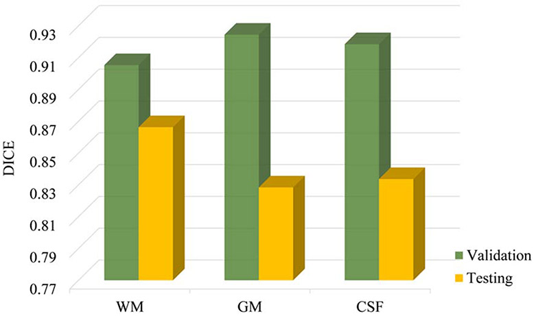
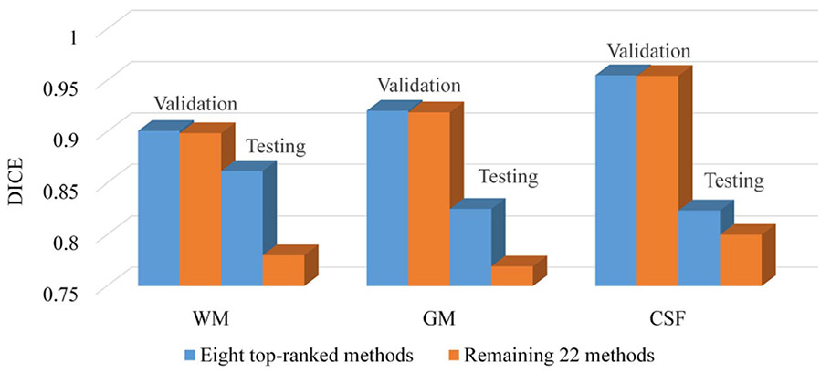
SEGMENTING infant brain images into different tissues, e.g., white matter (WM), gray matter (GM), and cerebrospinal fluid (CSF), is a vital step in the study of early brain development. Compared with adult brain images, infant brain images exhibit low tissue contrast, creating challenging tasks for tissue segmentation [1]. Therefore, existing tools developed for adult brains, e.g., SPM [2], CIVET [3], BrainSuite [4], FSL [5], FreeSurfer [6], and HCP pipeline [7], often perform poorly on the infant brain images. In fact, due to the inherent ongoing brain myelination and maturation [8]-[10], there are three distinct phases in the first-year brain MRIs [11], including (1) infantile phase (≤4 months), (2) isointense phase (5-8 months), and (3) early adult-like phase (≥9 months). Compared with the infantile and early adult phases, infant subjects in the isointense phase (e.g., 6 months old) exhibit the extremely low tissue contrast, resulting in the great challenge in tissue segmentation. Currently, available infant brain MRI processing pipelines, e.g., dHCP minimal pipeline [12] and Infant FreeSurfer [13], only focus on the infantile phase or early adult phase. To the best of our knowledge, there are very few works that can handle the isointense phase, e.g., iBEAT V2.0 Cloud (http://www.ibeat.cloud). To draw researchers’ attention to the segmentation of isointense infant brain MRI, we organized a MICCAI grand challenge on 6-month-old infant brain MRI segmentation from a single site: the iSeg-2017, http://iseg2017.web.unc.edu/. In the iSeg-2017 [1], we found that deep learning-based methods have shown their promising performance on 6-month-old infant subjects from a single site. However, data from multiple sites poses a number of challenges for the learning-based segmentation methods. Generally, the trained model may handle the testing subjects from the same site as the training subjects very well. However, the model often performs poorly on testing subjects from other sites with different imaging protocols/scanners, which is called the multi-site issue. Factors include equipment manufacturer, magnetic field strength, and acquisition protocol, which can affect image contrast/pattern and intensity distribution. One example is shown in Fig. 1 that learning-based methods achieve high accuracy on the validation subjects that are from the same site as the training subjects. Unfortunately, when the testing subjects are from other sites with different protocols/scanners (Table I), there is a significant decrease in performance in terms of Dice coefficient (DICE) metric (WM: from 0.90 to 0.86; GM: from 0.92 to 0.82; CSF: from 0.92 to 0.83). The multi-site issue hinders the popularity and practicability of learning-based methods. Currently, there are few challenges have been organized to explore this issue, (e.g., PROMISE12 [14], and M&Ms challenge [15]), and researchers proposed few-shot learning [16], domain adaptation [17], [18], transfer or distributed transfer learning [19], and adversarial learning [20], to deal with the multi-site issue. These existing methods still require either a small number of manual labels (annotations) from other sites for fine-tuning or a large number of images from other sites for adaptation. However, the annotation from other sites is prohibitively time-consuming and expensive, and usually only a small number of images are acquired in a pilot study before real-world medical applications are carried out.

Fig. 1.

Dice values from the 8 top-ranked methods on the validation and testing datasets in the iSeg-2019 challenge (the higher the DICE, the better the accuracy). Due to the multi-site issue, learning-based models often perform well on the validation subjects from the same site with the training subjects, whereas perform poorly on the testing subjects from other sites with different imaging protocols/scanners.

TABLE I.

Dataset Information of the iSeg-2019 Challenge. F: Female; M: Male

	Site	Scanner	Modality	TR/TE (ms)	Head Coil	Resolution (mm3)	Number of Subjects	Number of Subjects with Follow-up
Training	UNC (MAP)	Siemens (3T)	T1w	1900/4.4	32-channel	1.0×1.0×1.0	10 (5F/5M)	10
Validation			T2w	7380/119		1.25×1.25×1.95	13 (7F/6M)	0
Testing	UNC/UMN (BCP)	Siemens (3T)	T1w	2400/2.2		0.8×0.8×0.8	6 (3F/3M)	0
			T2w	3200/564		0.8×0.8×0.8
	Stanford University	GE (3T)	T1w	7.6/2.9		0.9×0.9×0.8	5 (3F/2M)	0
			T2w	2502/91.4		1.0×1.0×0.8
	Emory University	Siemens (3T)	T1w	2400/2.2		1.0×1.0×1.0	5 (2F/3M)	0
			T2w	3200/561		1.0×1.0×1.0

To attract more researchers to address the multi-site issue, in 2019, we organized a MICCAI grand challenge on 6-month infant brain MRI segmentation from multiple sites: iSeg-2019, http://iseg2019.web.unc.edu. Although a naive way is to train models based on multiple sites with different imaging protocols/scanners, the combinations of protocols/scanners are infinite. There is no way to include every possible case. Therefore, the goal of the iSeg-2019 is to promote training models based on one site to fit for all sites. Note that the iSeg-2019 is a follow-up challenge of the iSeg-2017 [1] in which the training and testing subjects are from the same site. In the iSeg-2019, the training subjects are randomly chosen from Multi-visit Advanced Pediatric (MAP) Brain Imaging Study [21] and the testing subjects are from three sites: University of North Carolina at Chapel Hill/University of Minnesota (Baby Connectome Project, BCP), Stanford University, and Emory University. It is worth noting that the imaging parameters/scanners from the three testing sites are different from the training dataset, with their imaging protocols/scanners listed in Table I. At the time of writing this paper, 30 teams have submitted their segmentation results to the iSeg-2019 website. In the next section, we introduce the cohort employed for this challenge. In Section III, we introduce 8 top-ranked methods in detail. Section IV and V elaborate on the performance, limitations and possible future directions, and Section VI concludes the challenge.

II. Multi-Site Datasets

Since the iSeg-2019 challenge aims to promote automatic segmentation algorithms on infant brain MRI from multiple sites, we select MR images from four different sites as training, validation, and testing datasets, respectively. Note that the training images and validation images are from the same site. To maximally alleviate bias effects caused by non-algorithmic factors, we employed the same selection criteria and the same preprocessing. Specifically, all subjects were randomly selected from normally developed infants without any pathology, and all scans were acquired at an average age of 6.0 (±0.8) months. Then, the same standard imaging preprocessing steps were performed, including resampling the resolution of all images into 1.0 × 1.0×1.0 mm³, skull stripping [22], intensity inhomogeneity correction [23], and removal of the cerebellum and brain stem. Finally, each preprocessed image was examined, and errors of skull stripping/removal of cerebellum/brain stem were manually corrected by experts (Dr. Li Wang and Dr. Valerie Jewells), which took us 2~3 minutes for each subject.

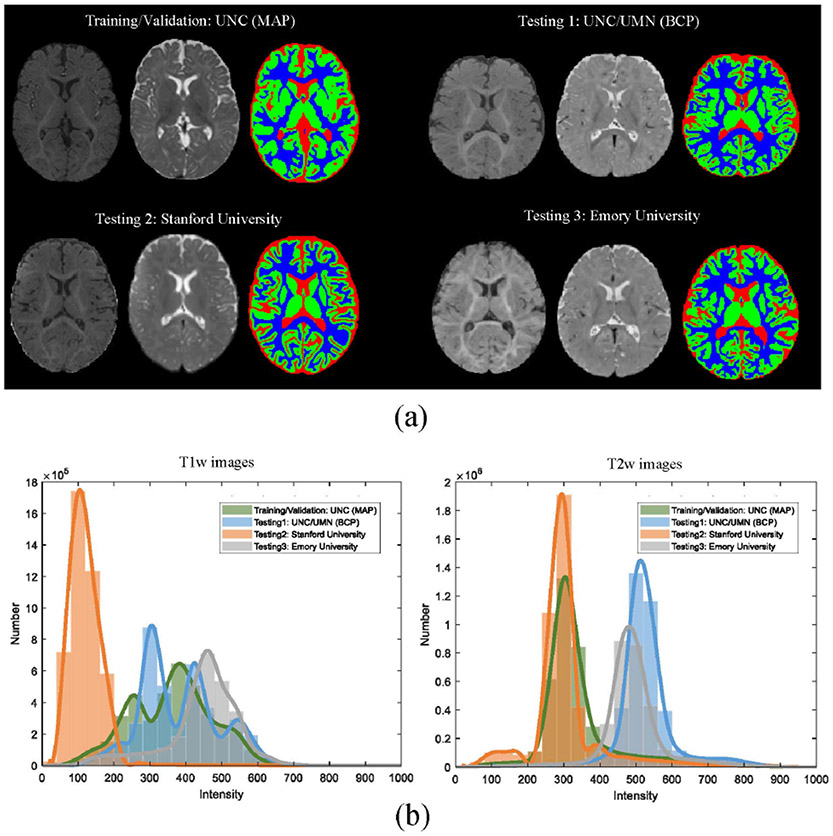
For training and validation, MR scans were chosen from MAP Brain Imaging Study. For testing, MR scans were randomly chosen from three sites, i.e., UNC/UMN (BCP), Stanford University, and Emory University. Detailed imaging protocols and scanners about datasets are listed in Table I. Specifically, the number of subjects from the MAP is 23, and the number of subjects from BCP, Stanford University, and Emory University is 6, 5, and 5, respectively. The reason for the different numbers from different sites is that more subjects have been collected in the MAP while fewer subjects are available from the testing sites, before kicking off the iSeg-2019. Therefore, for the MAP, we have enough time to perform manual annotations and more subjects were selected from the MAP. For the testing sites, both the number of available subjects and time for manual annotations are limited, and thus relatively fewer subjects were selected. All sites utilized Siemens scanners except for Stanford University which utilized a GE scanner. Furthermore, Fig. 2(a) shows T1w images, T2w images and manual segmentations of WM, GM, and CSF of 6-month infant subjects from four sites, and Fig. 2(b) plots average intensity distributions of T1w and T2w images from four sites. There are large differences in the intensity distributions and histogram shapes for the T1w images from Stanford University, compared to the other sites. These differences cause significant challenges for learning-based methods.

Fig. 2.

T1w and T2w MR images of infant subjects scanned at 6 months of age (isointense phase) from four sites with different imaging protocols/scanners, i.e., UNC (MAP), UNC/UMN (BCP), Stanford University, and Emory University, provided by the iSeg-2019. (a) Intensity images and the corresponding manual segmentations from each site. From left to right: T1w MR image, T2w MR image, and manual segmentation. (b) Average intensity distribution of T1w and T2w images from four sites marked by different colors. Note that the results are from the 8 top-ranked methods on all training/validation and testing datasets in the iSeg-2019 challenge.

Reliable manual segmentations were generated for training and quantitative comparisons. For all training subjects (with follow-up scans), a longitudinal guided segmentation algorithm [24] was applied to generate an initial segmentation. For all validation/testing subjects, due to the unavailability of follow-up scans, we used an anatomy-guided densely-connected U-Net [25] to generate an initial segmentation. The initial segmentations were later followed by manual correction under the guidance of an experienced neuroradiologist (Dr. Valerie Jewells, UNC-Chapel Hill). Details of the manual protocol are available in [26]. To maximally alleviate the potential bias from the automatic segmentations, we have spent considerable effort (20±5 hours) on the manual correction for each subject, with 200,000±10,500 voxels (25%±1.3% of total brain volume) corrected. To validate the quality of the manual segmentations, WM/GM scale analysis for total 39 subjects is listed in Appendix¹ Table X, based on a universal scaling law between WM and GM of the cerebral cortex [27], i.e.,

$$(1.23\pm 0.01){\log }_{10}\text{GV}-{\log }_{10}\text{WV}\approx 1.47\pm 0.04$$

where WV and GV are the volumes of WM and GM, respectively. We find that WM/GM scales from 38 out of 39 subjects are exactly within or highly close to the range [1.43, 1.51], indicating a high quality of manual segmentations. Although we have tried our best, the manual delineation from postmortem MRIs, providing a golden standard for tissue segmentation, is highly worth investigating.

As shown in Fig. 2(a), brain MRIs were manually segmented into WM, GM, and CSF, where myelinated and unmyelinated WM is marked blue, cortical and subcortical GM is marked green, and extracerebral/intraventricular CSF is marked red. Finally, we provided 10 infant subjects for training, 13 infant subjects for validation, and 16 infant subjects from three different sites for testing, as detailed in Table I. Note that the manual segmentations of training subjects were provided, together with the T1w and T2w images. While manual segmentations of validation/testing subjects are not provided to the participants. The segmentation results for the validation/testing dataset can be submitted maximally 3 times for evaluation and only the latest/best results were recorded.

III. Methods and Implementations

A total of 30 teams successfully submitted their results to the iSeg-2019 before the official deadline. We describe all participating teams with affiliations and key features used in their methods in Appendix Table I. Furthermore, we summarize the performance of all methods in Appendix Table II and find that one out of 29 methods did not utilize a deep learning technique. In the 28 methods using convolutional neural networks, 22 methods adopted the U-Net architecture, which is a strong baseline for medical image segmentation. It should be noted that, to alleviate the site differences, various domain adaptation strategies are employed in top-ranked methods, such as random intensity adjustment in QL111111 and xflz, and global feature alignment in SmartDSP. More details are illustrated in the following description and are further concluded in Table III. According to the performances of different methods, the domain adaptation is helpful in dealing with site differences. In this section, we will introduce the metric of selecting the 8 top-ranked methods and further describe these 8 top-ranked methods according to their ranking order, with the corresponding source codes listed in Appendix Table X.

TABLE III.

Comparisons of the Eight Top-Ranked Methods in the iSeg-2019 Challenge

TEAM	Architecture	Tool	How to deal with site differences?	Key highlight	Augmentation	Training Loss	2D/3D Patch size (training/testing)
QL111111	Self-attention and multi-scale dilated 3D UNet	Tensorflow	Intensity adjustment	Attention mechanism +multi-scale	No	Cross-entropy	3D (32×32×32)
Tao_SMU	Attention-guided Full-resolution Network	Tensorflow	Training data augmentation, contrast and lightness adjustment	Full resolution + attention mechanism	Dimension transformation, contrast and lightness adjusting	Cross-entropy	3D (32×32×32)
FightAutism	3D UNet	Pytorch	Histogram matching	Automate designing of segmentation pipeline	Random rotation, scaling, mirroring, and gamma transformation.	Cross-entropy	3D (112×128×128)
xflz	Intensity-augmented 3D UNet	Tensorflow	Intensity adjustment	Intensity augmentation for adaptation of multi-site data	Intensity augmentation, gaussian nosie and flip	Cross-entropy	3D (64×64×64)
SmartDSP	Adversarial learning 3D UNet	Pytorch	Global feature alignment	Adversarial learning + automate designing of segmentation pipeline	-	Cross-entropy, dice loss and adversarial loss	3D (112×128×128)
CU_SIAT	Entropy Minimization 3D densely connected network	Pytorch	Distribution alignment	Adversarial entropy minimization strategy	-	Cross-entropy and adversarial loss	3D (64×64×64)
trung	Cross-linkedFC-DenseNet	Pytorch	-	Cross link + channel attention	-	Cross-entropy	3D (64×64×64)
RB	Dense residual 3D Unet	Pytorch	-	Dense block + residual connection	-	Cross-entropy and dice loss	3D (64×64×64)

Metric of selecting 8 top-ranked methods:

In the iSeg-2019 challenge, we adopted DICE, 95th-percentile Hausdorff distance (HD95), and average surface distance (ASD) [1] to evaluate the performance of participating methods. For each metric, we first rank the methods in terms of CSF, GM and WM segmentations, respectively. Then, we set the weights for each tissue type according to its normalized volume with the total brain volume and calculate the overall score for each method:

$$\begin{gathered} \text{Score}=\text{CSF/TV}{\text{(rank}}_{\text{CSF}-\text{DICE}}+{\text{rank}}_{\text{CSF}-\text{HD95}}+{\text{rank}}_{\text{CSF}-\text{ASD}}) \\ +\text{GM/TV}{\text{(rank}}_{\text{GM}-\text{DICE}}+{\text{rank}}_{\text{GM}-\text{HD95}}+{\text{rank}}_{\text{GM}-\text{ASD}}) \\ +\text{WM/TV}{\text{(rank}}_{\text{WM}-\text{DICE}}+{\text{rank}}_{\text{WM}-\text{HD95}}+{\text{rank}}_{\text{WM}-\text{ASD}}) \end{gathered}$$

where the total brain volume TV is equal to the volumes of CSF + GM + WM, and rank_{{CSF,GM,WM}–{DICE,HD95,ASD}} is the rank of different tissue types in terms of DICE, HD95, and ASD. Finally, we select 8 top-ranked methods according to their overall scores, as listed in Appendix Table XI.

A. QL111111: Northeastern University, China

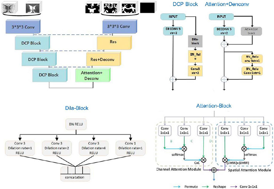
Lei et al. propose a novel method based on a 3D U-Net combined with an attention mechanism [28]. To deal with the site differences between training images and testing images, they set random contrast to 4.64~4.66 for T1w images, and 1.34~ 1.36 for T2w images. They further apply gamma correction for T2w images. Then both T1w and T2w images are standardized and cropped to 32 × 32 × 32 patches as input to the network, as presented in Fig. 3. The residual-network-based structure used in the downsampling path consists of three dilated convolution pyramid (DCP) blocks. The left side of the DCP block includes a 1 × 1 × 1 convolutional layer, and the right side contains a dila-block module, an activated convolutional layer with a convolution kernel size of 3 × 3 × 3 and a stride of 2. This dila-block consists of four dilated convolutions and each dilated convolution includes a pre-activation layer, which is concatenated and passed to the next stage. In the upsampling path, self-attention is utilized to capture long-range dependencies, that is, to aggregate the information of feature maps. The contributions of their work can be summarized as follows: (1) They utilize the convolutions with different dilation rates to effectively capture multi-scale information. (2) An attention method is proposed to effectively encode the wider context information and mine the interdependencies between channel maps.

Fig. 3.

Team QL111111: the structure of 3D U-Net based on attention mechanism.

Leave-one-out cross-validation is used for training/validation. During testing, 10 leave-one-out cross-trained models are applied, and a majority voting is performed to get the final segmentation. The optimization of network parameters is performed via Adam optimizer. Learning rate is initialized as 3.3e-3 and weight decay is set as 2e-6. Their method is implemented in Python using TensorFlow framework. Experiments are performed on a computational server with one NVIDIA 1080Ti with 11GB of RAM memory. It takes about 3 hours for training and 2 minutes for testing each subject.

B. Tao_SMU: Southern Medical University, China

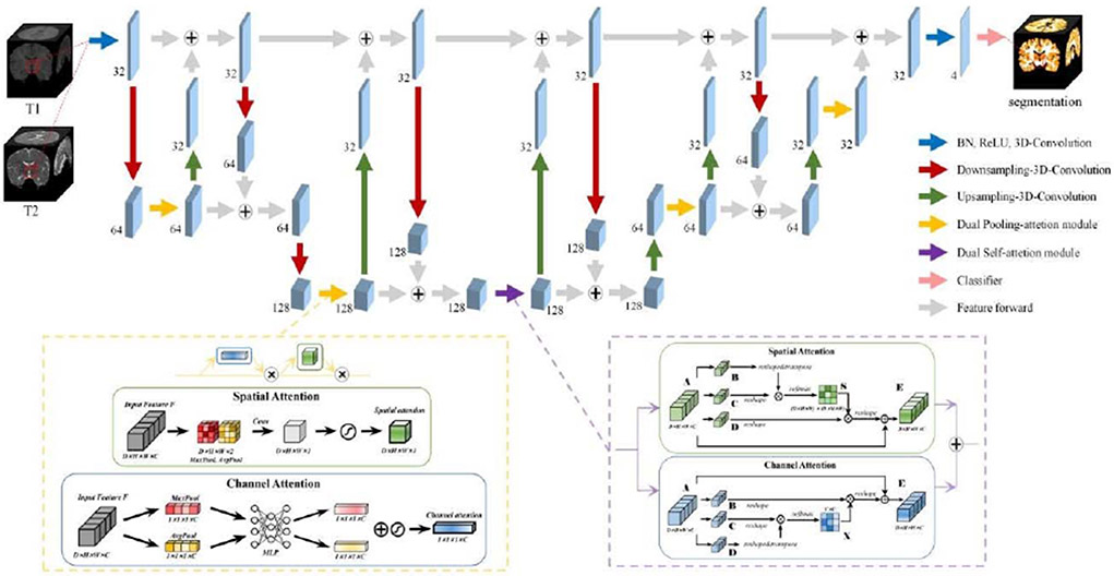
Zhong et al. propose an attention-guided full-resolution network for segmentation of 6-month infant brain MRIs, which is extended from the full-resolution residual network [29] and attention mechanism [30]. The network consists of a 3D two-stream full-resolution structure and two types of 3D attention modules, including Dual Self-Attention Module and Dual Pooling-Attention Module. First, to address spatial information loss, a 3D-based full-resolution architecture is constructed to preserve high-resolution information by keeping a separate high-resolution processing stream. Second, this architecture is combined with an attention mechanism to capture global relationship and generate more discriminative feature representations through spatial and channel axes. To deal with large differences between training images and testing images from multiple sites, they augment the training data with two strategies. First, they transform each subject from different dimensions, i.e., transpose each subject by swapping 3 axes in different combination, to generate 5 new subjects, thus providing more features from different views. Second, they randomly adjust the contrast and lightness for each training subject using the parameter ±20%.

The proposed architecture is detailed in Fig. 4. The two-stream structure combines multi-scale context information using two processing streams. The resolution stream carries information at full resolution for precise segmentation of boundaries. The semantic stream acquires high-level features for class identification. In this model, stride size is set as 2 or 4 to achieve magnification/reduction of feature maps 2 or 4 times. Except for the last convolutional layer for classification, all convolution and deconvolution sizes are set as 3 × 3 × 3. During the entire process, exchanging feature information between the two streams execute repeated multi-scale fusion. Meanwhile, two types of attention mechanism are used to improve model feature extraction capabilities. In the bottom block, the fusion features pass through Dual Self-Attention Module to obtain attention-guided features grabbing the global dependencies. In the block of the upsampling and downsampling processes, after passing through the convolution or deconvolution layer to downsample or upsample, the fused features are processed by Dual Pooling-Attention Module to obtain attention-guided features. The motivation for this allocation comes from the different computational costs required by the two attention mechanisms. Dual Pooling-Attention Module is lighter, less expensive, and easier to implant into every part of the model, whereas Dual Self-Attention Module requires more computing resources, but provides a stronger ability to capture global dependencies. Both attention modules include spatial-based and channel-based parts, which can selectively aggregate contexts based on spatial attention maps, and at the same time emphasize class-dependent feature maps, helping to enhance the channel distinguishability of original features. Finally, a classifier with 1 × 1 × 1 convolution is used to classify the feature maps into target classes.

Fig. 4.

Team Tao_SMU: the proposed attention-guided full-resolution network architecture.

The training input of the network is 32 × 32 × 32 × 2 patches of T1w and T2w images. Both of them are normalized to zero mean and unit variance. The network is trained with Adam optimizer on the cross-entropy loss, using minibatches of 4. During prediction, the step size is set as 4. It takes about 48 hours for training and 12 minutes for segmenting each subject on a TitanX Pascal GPU and Tensorflow framework.

C. FightAutism: Nanjing University of Science and Technology, China

To deal with large differences between training images and testing images from multiple sites, Jun et al. employ histogram matching to alleviate the intensity variance from multiple sites. Specifically, the intensity distributions of all testing subjects are adjusted to align one randomly selected subject from the validation dataset.

The employed architecture is a 3D U-Net [31] which consists of one downsampling path and one upsampling path. Each path includes 5 convolution blocks and each block comprises of 3 × 3 × 3 convolution layer, instance normalization layer and leaky rectified linear unit. Long skip connections are also used in the same resolution between downsampling and upsampling paths.

Both T1w and T2w images are used to train the U-Net. The pre-processing includes foreground (non-zero regions) cropping and Z-Score normalization. All 10 training subjects are used for training. Data augmentation includes random rotation, scaling, mirroring, and gamma transformation. The optimizer is Adam with an initial learning rate of 3e-4. During testing, test time augmentation is employed by mirroring along all axes. The implementation is based on PyTorch and nnU-Net [32].

D. Xflz: Children’s National Medical Center, USA

Feng et al. propose an optimized 3D U-Net with tissue-dependent intensity augmentation for segmentation of 6-month infant brain MRIs. To deal with the site differences, they use a tissue-dependent intensity augmentation method to simulate the variations in contrast. To emulate the inconsistent of contrast, the intensity of each tissue (i.e., WM, GM, and CSF) is multiplied by different factors during training.

The network structure is based on a 3D U-Net. The encoding path includes three blocks with each block containing two 3×3×3 convolution layers and one 3D max-pooling layer. Two additional convolution layers are added at the bottom. Three decoding blocks are used with long range connection from the corresponding encoding block. Parametric rectifier (PReLU) is used instead of conventional rectifier (ReLU). Compared with the original U-Net for 2D images, the number of features is increased to capture more 3D information, yielding a wider network. As the input of the network, T1w and T2w images are concatenated; the output is the probabilistic maps of WM, GM, CSF, and background.

During each iteration of training, after reading the original T1w and T2w images and the label map, the intensities at each region are multiplied by different factors randomly sampled from 0.9 to 1.1 using a uniform distribution to simulate the effect of different imaging protocols. Randomly sampled Gaussian noise with different standard deviations is then added to the resulting T1w and T2w images, respectively. Furthermore, to simulate the symmetry of the left and right brain hemispheres, the images are randomly flipped. A patch of 64 × 64 × 64 × 2 is randomly extracted from the original images and fed to the network. The model is trained on the provided data for 4000 epochs and the total time was about 7.5 hours on an NVIDIA Titan Xp GPU. During deployment, a sliding window approach is used with a stride of 16 and for each voxel, the final probability is obtained by averaging all outputs from overlapping patches. No post-processing is performed. The deployment time is about 1 minute per case.

Although the method achieves good performance in the validation dataset, the performance declines on the multi-site testing dataset, indicating that the augmentation method is not sufficient to fully emulate the imaging differences. As the imaging parameters including TR and TE are available, they also try to use a more complex model based on MR physics to simulate the images using different sets of protocols; however, as the MR sequence is very complicated, only using TR, TE, T1w and T2w information and a simple signal decay model fails to yield realistic images. For simplicity and robustness, they just randomly scale the regional intensities differently.

E. SmartDSP: Xiamen University and The Chinese University of Hong Kong, China

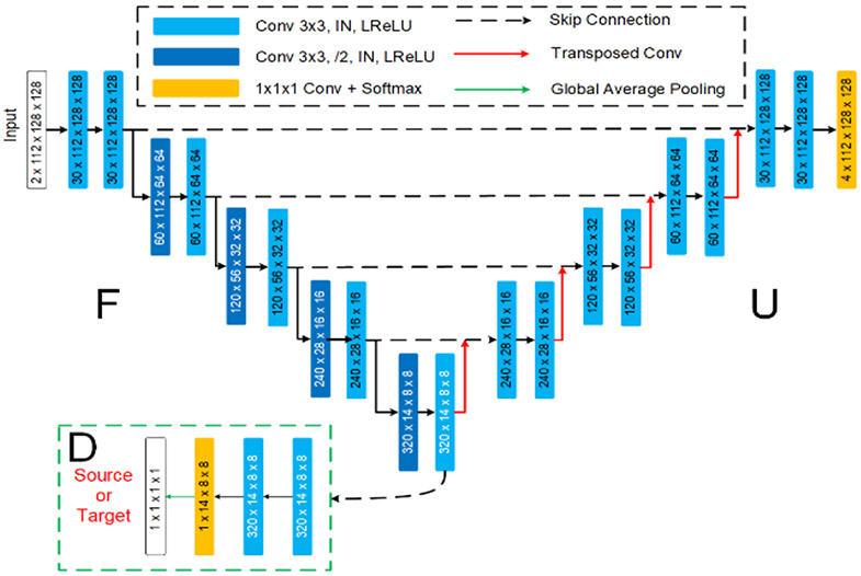
Ma et al. propose a framework with adversarial learning of unsupervised cross-domain global feature alignment based on nnU-Net [32]. The nnU-Net is employed [32] as the backbone, and the architecture of Ada-nnUNet model is shown in Fig. 5. Inspired by [33] and [34], the network utilizes a feature-level domain discriminator at the bottleneck layer of nnU-Net, for aligning the distributions of target features and the source features in a compact space. By assuming the training dataset as source domain, and the unlabeled testing dataset as target domain, they formulate the problem as an unsupervised domain adaptation task. Specifically, the feature-level discriminator block consists of two 3 × 3 convolutional layers and one 1 × 1 convolutional layer. Then, the feature maps are forwarded to a global average pooling layer. This domain discriminator is trained to predict the domain of input features in a highly abstracted feature space, by practically setting the domain label as one for the source domain and zero for the target domain. By denoting F_θ as the feature extraction downsampling layers before the bottleneck layer, U_ϕ as the upsampling layers of the segmenter, and D_ψ as the feature-level domain discriminator, the overall objective of the network is:

$$\underset{D_{\psi }}{\max }\underset{F_{\theta },U_{\varphi }}{\text{min}}{\mathcal{L}}_{task}(F_{\theta },U_{\varphi })+{\mathcal{L}}_{adv}(F_{\theta },D_{\psi })$$

where ${\mathcal{L}}_{task}$ is the task loss which is the sum of dice loss and cross-entropy loss. For the loss of feature-level domain discriminator, they expect the classifier to alleviate the imbalance of alignment difficulties across different samples, they follow [34] and apply the focal loss for ${\mathcal{L}}_{adv}$ as:

$$\begin{gathered} {\mathcal{L}}_{adv} \\ =-\frac{1}{N_s}{\sum }_{i=1}^{N_s}{\left(1-D_{\psi }\left(F_{\theta }\left(x_s^i\right)\right)\right)}^{\gamma }\log \left(D_{\psi }\left(F_{\theta }\left(x_s^i\right)\right)\right) \\ =-\frac{1}{N_t}{\sum }_{i=1}^{N_t}{\left(D_{\psi }\left(F_{\theta }\left(x_t^i\right)\right)\right)}^{\gamma }\log \left(1-D_{\psi }\left(F_{\theta }\left(x_t^i\right)\right)\right) \end{gathered}$$

where N_s denotes the number of source examples and N_t denotes the number of target examples, and each training sample drawn from source domain and target domain is represented by $x_s^i$ and $x_t^i$, respectively. The γ adjusts the weight on hard-to-classify examples and was empirically set as 5.0 in the network. In each training batch, source image $x_s^i$ is also forwarded to minimize the segmentation network for ${\mathcal{L}}_{task}$.

Fig. 5.

Team SmartDSP: the proposed Ada-nnUnet network.

The network is implemented by using the PyTorch library, with Adam optimizer. The initial learning rate is set as 3e–4 and the weight decay regularizer is set as 3e–5. The inputs of the network contain T1w and T2w MR images without extra training dataset. In the training stage, patches with a size of 112 × 128 × 128 are randomly extracted from the volumes and input to the network. The training procedure takes around two days on a GPU of NVIDIA Titan Xp with 12 GB memory and it takes around 10 seconds to process one subject during the testing phase. The potential limitation of Ada-nnUNet is that the feature-level alignment is imposed only in the coarse feature space. In this regard, some detailed information would have to be neglected during adversarial distribution alignment, which may impede segmentation performance.

F. CU_SIAT: The Chinese University of Hong Kong and Shenzhen Institutes of Advanced Technology, China

To deal with the large differences between training images and testing images from multiple sites, Yu et al. adopt an Entropy Minimization Network (EMNet) to conduct unsupervised domain adaptation to align distributions between training and testing datasets.

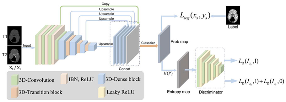
As shown in Fig. 6, the proposed framework contains two main components: segmentation network and discriminator network. For the segmentation part, they employ the 3D densely connected network [35] to predict the brain structures by taking the T1w and T2w images as inputs. To enhance the generalization capability of the network over different site data, they carefully integrate Instance Normalization (IN) and BN as building blocks of the segmentation network [36]. The so-called “IBN” layer design can improve the network performance across multiple site data. Moreover, a discriminator network is adopted to align the distributions between training and testing datasets by adversarial entropy minimization [37]. In the problem setting, the training dataset is regarded as a source domain and the testing dataset is treated as a target domain. They firstly compute the entropy maps of segmentation predictions for the source and target domain, respectively. These entropy maps are fed into the discriminator network to produce domain classification outputs. The whole framework is trained with adversarial learning: the discriminator network is trained to distinguish the inputs from the source or target domain, while the segmentation network is trained to generate similar predictions for the source and target domain data to fool the discriminator network. Specifically, the optimization objective for the segmentation network can be written as:

$$\underset{\theta s}{\text{min}}\frac{1}{\mid {\chi }_s\mid }\sum _{x_s}{L}_{seg}(x_s,y_s)+{\lambda }_{adv}\frac{1}{\mid {\chi }_t\mid }\sum _{x_t}{L}_D(I_{x_t},1)$$

and the objective of discriminator network is

$$\underset{\theta D}{\text{min}}\frac{1}{\mid {\chi }_s\mid }\sum _{x_s}{L}_D(I_{x_s},1)+\frac{1}{\mid {\chi }_t\mid }\sum _{x_t}{L}_D(I_{x_t},0)$$

where θ_S and θ_D denote parameters of segmentation and discriminator network, respectively. χ_s and χ_t represent the set of source and target examples, I_xs and I_xt denote entropy maps of corresponding images. The L_seg(x_s, y_s) and L_D(I_xt, 1) are cross-entropy losses and adversarial loss to train the segmentation network, and λ_adv is used to balance the weights of the two losses.

Fig. 6.

Team CU_SIAT: the architecture of entropy minimization network (EMNet). The segmentation network is based on 3D densely connected network with IBN layer. An adversarial entropy minimization strategy is used to minimize the self-information (i.e., entropy map) H(P) distribution gap between source and target domains.

The segmentation and discriminator network are all trained with Adam optimizer with a mini-batch size of 4. The learning rate is initially set as 2e-4 and decreased by a factor of β = 0.1 every 10000 iterators. They train 35000 iterations. The λ_adv is set as 0.001. They use 10 labeled training subjects and 16 unlabeled testing subjects to train the whole framework. Due to the limited GPU memory, sub-volume of size 64 × 64 × 64 is used as network input. In the testing phase, they employ the sliding window strategy to generate the whole probability map of each test volume. Note that the discriminator network is abandoned during the testing phase. Generally, it takes about 24 hours to train the model and about 8 seconds to test one object on a GeForce RTX 2080Ti GPU with PyTorch library.

G. Trung: Media System Laboratory, Sungkyunkwan University, South Korea

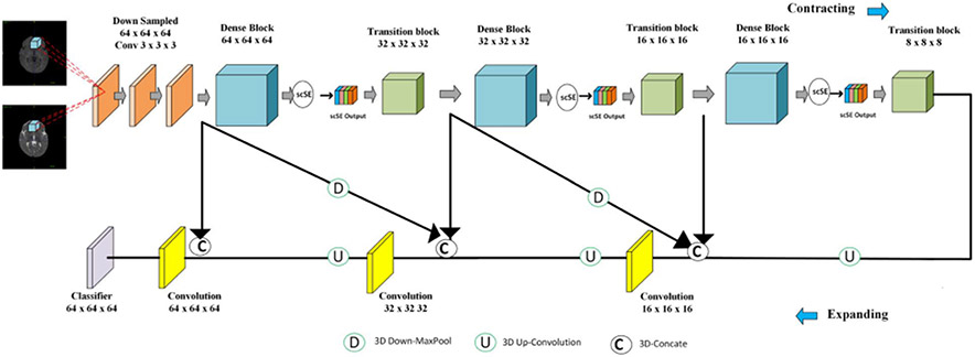
Trung et al. introduce a segmentation method for 6-month infant brain MRIs, called Cross-linked FC-DenseNet (cross-linked fully convolution-DenseNet), as shown in Fig. 7. First, following each Dense block, an end-to-end concurrent spatial and channel squeeze & excitation (scSE) is added [38], which allows the model to explore the interdependency among channels. Second, 3D FC-DenseNet is combined with the cross-links (such as downsampling links) [39] to learn more features from the contracting process.

Fig. 7.

Team trung: the proposed cross-linked FC-DenseNet architecture for volumetric segmentation.

The network consists of two paths: a contracting path and an expanding path. The initial part of the network has three 3 × 3 × 3 convolutions with stride 1 followed a batch normalization layer (BN) and a ReLU that generates 64 output feature maps. The contracting path with three dense blocks with a growth rate of k = 16 [35] is exploited. Each dense block has four BN-ReLU-Conv(1 × 1 × 1)-BN-ReLU-Conv (3 × 3 × 3). To alleviate the over-fitting after this Conv (3 × 3 × 3), they use a dropout layer with a dropout rate of 0.2 [40]. After each dense block, they add scSE block [38] to explore the interdependencies between the channels. After scSE block, the transition block includes BN-ReLU-Conv (1 × 1 × 1)-BN-ReLU followed by a convolution layer of stride 2 to reduce feature map resolutions while preserving the spatial information [38]. Meanwhile, for recovering the feature resolution, the expanding path has three convolution layers. They resize the outputs of the first and last transition block using max pooling and up-convolution of 2 × 2 × 2 by stride 2 to get an equal resolution with the second transition output and concatenate all of them as input of the third convolution layer. Also, the convolution layer uses three different sizes of feature maps: the output of the initial part, the output of the first transition block, and the output of the third convolution layer. Otherwise, they use two different sizes of feature maps in the first convolution layer: the output of the initial part, and the output of the second convolution layer. This cross-link path allows the model to capture multiple contextual features from the different layers and improves a gradient flow. Finally, a classifier consisting of ReLU-Conv (1 × 1 × 1) is used to classify the concatenation feature maps into target classes.

They implement and train the proposed network with an NVIDIA Titan XP and Pytorch library. First, they randomly crop sub-volume samples with size 64 × 64 × 64 voxels. The network is trained with an Adam optimizer and 6000 epochs with a mini-batch size of 2. The learning rate and weight decay are set to 0.0002 and 0.0006, respectively. They use nine subjects for training and one subject for validation from the iSeg-2019 training dataset. It takes about 40 hours for training and 6 minutes for testing each subject.

H. RB: Concordia University, Montreal, Canada

Based on the U-Net architecture [31], Basnet et al. propose a 3D deep convolutional neural network. The difference between U-Net and the proposed architecture is the utilization of densely connected convolutional layers as building blocks of contracting the path and residual skip connections between contracting and expanding paths in the latter.

Figure 8 shows the proposed network architecture. The contracting path begins with 3 sequential 3 × 3 × 3 convolutional layers with 32 kernels. The convolutional layer is followed by BN and a ReLU. Then, 4 downsampling dense blocks are stacked to halve the feature resolution at each block and gradually capture the contextual information. Each dense block has 8 convolution layers and starts with a max-pooling layer as shown in Fig. 9. In the dense block, every convolutional layer is preceded by a BN-ReLU. After each pair of convolutional layers in the block, a dropout layer with a dropout rate of 0.2 is used to reduce overfitting. The output feature maps of each pair are concatenated with that of the previous pairs forming the dense connections. The first convolutional layer in the pair has 64 kernels of size 1 × 1 × 1 and the second one has 16 kernels of size 3 × 3 × 3. After every dense block, a 1 × 1 × 1 convolutional layer preceded by BN-ReLU called the transitional block is used to halve the number of feature maps. In the expanding path, 4 bilinear upsampling layers are applied to double the feature resolution and halve the number of feature maps. A transitional block is used after each upsampling layer to match the number of feature maps to that of the transitional blocks in the contracting path of the same resolution. The corresponding feature maps from contracting and expanding paths are elementwise summed using skip connections. At the end of the fourth transitional block of expanding path, the output features of the third convolutional layer from the beginning of the contracting path are added and fed to a 1 × 1 × 1 convolution layer preceded by BN-ReLU to get probability scores for the four output channels: WM, GM, CSF, and background. The proposed network has 625,926 learnable parameters with 48 layers.

Fig. 8.

Team RB: the network architecture for U-DenseResNet.

Fig. 9.

Dense block used in Fig. 8.

For training, the T1w and T2w images are normalized to zero mean and unit variance, and cropped to 64 × 64 × 64 patches as input. The network is trained using Adam optimizer on a combination of cross-entropy and dice loss, with minibatches of size 2 for 9600 epochs. The initial learning rate is set to 2e-4 and decreased by a factor of 0.1 after 5000 epochs. The method is implemented using the PyTorch library on a computer with Intel Core i5-9600K CPU @ 3.70GHz, 16GB RAM and an NVIDIA RTX 2070 GPU. It takes about 16 hours for training and 1 minute for testing each subject.

IV. Results and Discussion

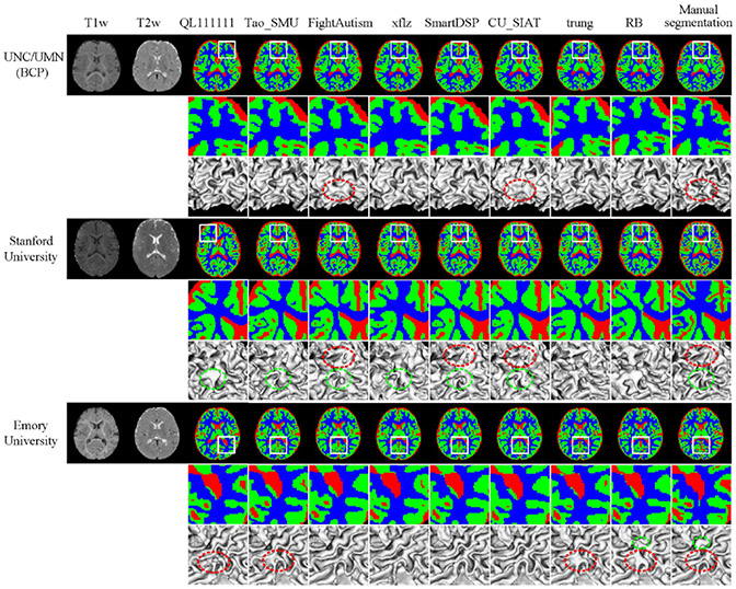
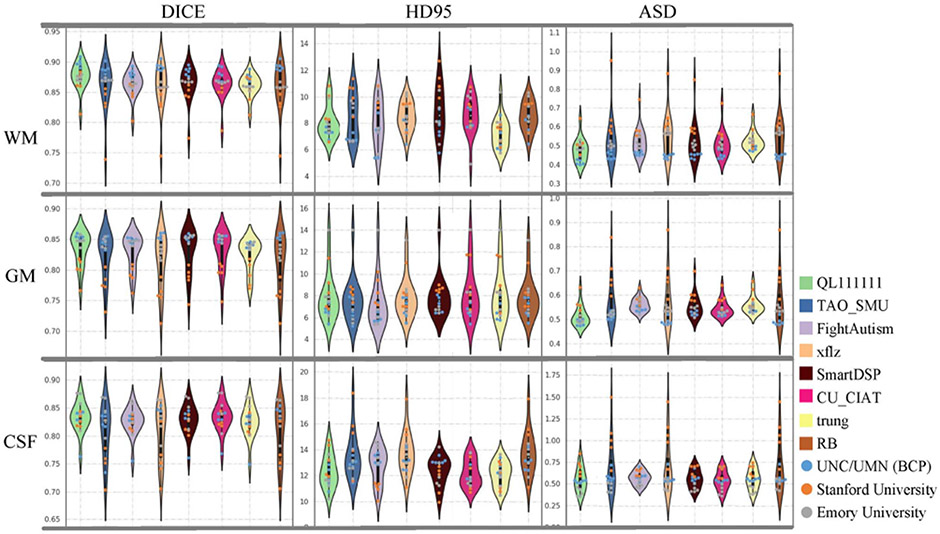
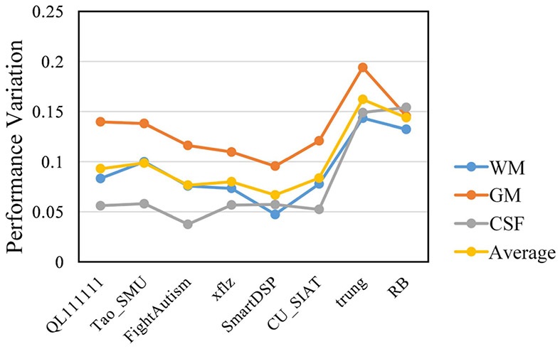
In this section, DICE, HD95, and ASD [1] are adopted to evaluate the performance. First, segmentation results of different teams are presented in Fig. 10. Evaluations in terms of the whole brain using DICE, HD95 and ASD are presented in Fig. 11 and Appendix Table III, respectively. For simplification, {WM, GM, CSF}-{DICE, HD95, ASD} denotes the performance on the soft tissue (WM, GM and CSF) in terms of a metric (DICE, HD95 and ASD). Besides evaluations for the whole brain, we also evaluate the performance based on small regions of interest (ROIs), gyral landmark curves and cortical thickness in Figs. 13, 14, and 15, Appendix Tables VII and VIII. To compare the difference of segmentation results among the 8 top-ranked methods, Wilcoxon signed-rank tests are calculated for statistical analysis in Appendix Table IV, V and VIII. Furthermore, Wilcoxon rank-sum tests are applied to analyze the statistically significant difference among multiple sites/teams in Appendix Table VI. In addition, Fig. 12 shows the performance variation of 8 top-ranked methods across three testing datasets. We also compare the 8 top-ranked methods and the remaining 22 methods on the validation dataset and testing dataset as shown in Fig. 16.

Fig. 10.

Segmentation results by 8 top-ranked methods on testing subjects from three sites. From left to right: T1w and T2w images, tissue segmentation results obtained by 8 top-ranked methods, and manual segmentations. Zoomed 2D segmentation results and corresponding 3D rendering results are also included, where dotted circles indicate significant incorrect results.

Fig. 11.

Performance of the 8 top-ranked methods on tissue segmentation, in terms of DICE, HD95 and ASD, using violin-plots. Testing subjects from three sites are marked as points in three colors.

Fig. 13.

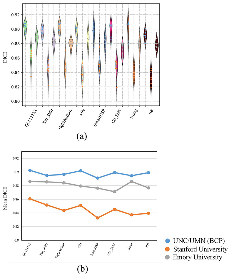
Performance of the 8 top-ranked methods on ROI-based evaluation. (a) The DICE values of each method on three testing sites. For the violin-plots, different color points indicate different sites. (b) The mean DICE values of each method on three testing sites.

Fig. 14.

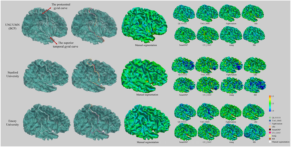
Two gyral curves (i.e., the superior temporal gyral curve and the postcentral gyral curve) and cortical thickness maps for 8 top-ranked methods and manual segmentations on three sites respectively. From left to right: manual delineation of two gyral curves, the gyral curves from the segmentation results of 8 top-ranked methods, cortical thickness maps of manual segmentations, and cortical thickness maps from the segmentation results of 8 top-ranked methods.

Fig. 15.

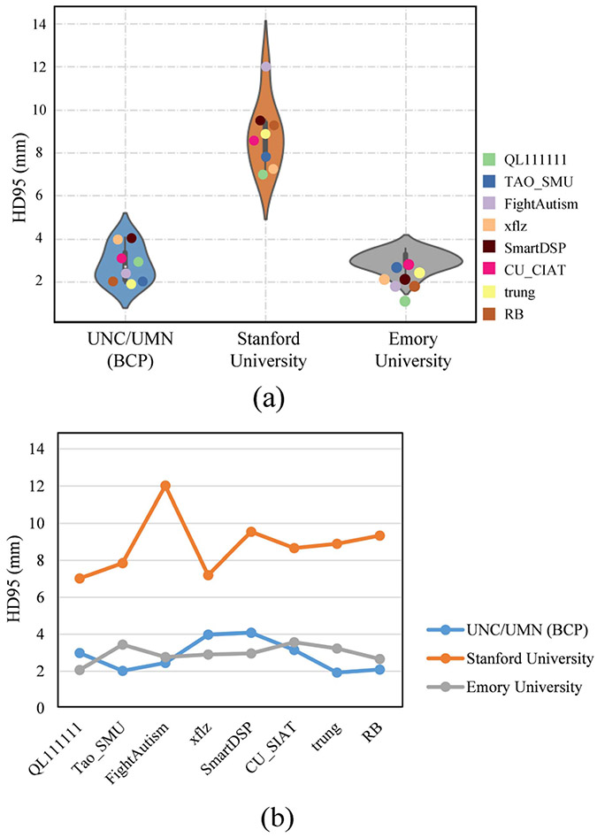
HD95 evaluation of 8 top-ranked methods on the superior temporal gyral curve and the postcentral gyral curve. (a) Violin-plot shows HD95 distribution for each testing site. (b) Line chart plots HD95 evaluation among three testing sites for each method.

Fig. 12.

The performance variation of 8 top-ranked methods across three testing sites.

Fig. 16.

The DICE values of 8 top-ranked methods and the remaining 22 methods on the validation dataset and testing dataset, respectively.

First, Fig. 10 qualitatively shows the segmentation results of different teams, and Appendix Table III quantitatively lists the performances in terms of DICE, HD95 and ASD. Fig. 11 further employs violin-plots to illustrate the performance distribution of each testing subject. Obviously, from Fig. 10, these methods consensually perform better on testing subjects from UNC/UMN (BCP) and Emory University sites, compared with Stanford University site. Then from the quantitative analysis in Appendix Table III, 7 out of 8 top-ranked methods achieve relatively better segmentation results on UNC/UMN (BCP) site in terms of three metrics, which can be also observed directly from Fig. 11. In Fig. 11, the light blue, orange, grey points, denote performance on the testing subjects from UNC/UMN (BCP), Stanford University, and Emory University, respectively. It can be seen the light blue points are always at the top location with regard to the DICE metric in the first column, while the orange points and grey points are located in the bottom and middle, respectively. As for HDF95 and ASD, the corresponding point location is opposite as shown in the second and third columns. We can conclude from the above analysis, in terms of the whole brain, most methods achieve the best performance on testing subjects from UNC/UMN (BCP) and the worst performance on those from Stanford University, while in between on those from Emory University.

Besides, the violin-plot shapes of QL111111, FightAutism and trung teams are wide with few outliers, indicating their relatively stable performance across three testing sites, as shown in Fig. 11. Furthermore, in order to compare the difference of segmentation results among the 8 top-ranked methods, Wilcoxon signed-rank tests are calculated as listed in Appendix Tables IV (on three sites totally) and V (on three sites separately) with an all-against-all diagram in terms of three metrics (i.e., DICE, HD95 and ASD). We can find that only QL111111 has a strongly statistically significant difference in WM-DICE and WM-ASD compared with other teams as listed in Table IV (p-value<0.01). However, from the separate evaluation on three sites reported in Appendix Table V, QL111111 only has weak statistical significance on WM-ASD when testing on UNC/UMN (BCP) site, and on WM-ASD when testing on Stanford University site (p-value<0.05). As for the HD95 metric, there is no statistically significant difference among these teams for the total or separate evaluation of three sites in Appendix Tables IV and V respectively (p-value>0.05). As for the ASD metric, QL111111 has statistically significant differences in terms of WM and GM with other teams on three sites totally as shown in Table IV (p-value<0.01), whereas from the separate analysis of three sites reported in Table V, it only has weak statistical significance on GM-ASD when testing on Emory University site (p-value<0.05).

To better reflect the performance of 8 top-ranked methods across multiple testing sites, Fig. 12 shows the corresponding performance variation $\mathbb{E}$, which is calculated by:

$$\mathbb{E}=\frac{1}{3}\ast (\mid D_{BCP}-D_{SU}\mid +\mid D_{BCP}-D_{EU}\mid +\mid D_{SU}-D_{EU}\mid )$$

where D_BCP, D_SU, and D_EU indicate the DICE values of participating methods on the testing subjects from UNC/UMN (BCP), Stanford University, and Emory University sites, respectively. For the 8 top-ranked methods of the iSeg-2019 challenge, the first 6 top-ranked methods adopted domain adaptation techniques, i.e., QL111111, Tao_SMU, FightAutism, xflz, SmartDSP, and CU_SIAT, while the remaining 2 methods did not adopt domain adaptation techniques, i.e., trung and RB. We can observe that, the first 6 methods present smaller performance variations across sites, compared with the last 2 methods. Besides, to better analyze the difference between top-ranked methods with or without domain adaptation, we calculate p-values between them in terms of DICE for WM (p-value<0.01), GM (p-value<0.05), and CSF (p-value<0.01), indicating statistically significant difference between the two groups. The reason is mainly due to the adoption of domain adaptation in the first 6 methods.

Second, to further compare the performance of the 8 top-ranked methods in respect of small ROIs, 80 ROIs-based evaluation is employed in this paper. Following our previous review article in the iSeg-2017 [1], we use a multi-atlas-based technique to parcellate each testing subject into 80 ROIs. In particular, two-year-old subjects from www.brain-development.org are employed as individual atlases, in which each case consists of a T1w MR image and the corresponding label image with 80 ROIs (excluding cerebellum and brainstem). First, each T1w MR image is segmented into WM, GM, and CSF tissues by iBEAT V2.0 Cloud (http://www.ibeat.cloud). Then, based upon the tissue segmentation maps, all anatomical atlases are warped into the space of each testing subject via ANTs [41]. Finally, each testing subject is parcellated into 80 ROIs using majority voting. Due to the large number of ROIs, we only employ the DICE metric to measure the similarity of automatic segmentations with the manual segmentation as listed in Appendix Table VII. In addition, we use the violin-plot in Fig. 13(a) to demonstrate the distribution of DICE values among three testing sites, where the different color points in the violin-plot indicate different testing sites. As shown in Fig. 13(a), the DICE values from the Stanford University site show a larger distribution range compared with the other two sites, which indicates segmentation performance of the methods across different sites is unstable. Furthermore, to further show the performance on each site, Fig. 13(b) calculates the mean DICE values of each site, which is consistent with Figs. 10 and 11, i.e., all of 8 top-ranked methods perform poorly on the Stanford University site due to its different imaging protocol/scanner.

Third, in human brains, gyri are part of a system of folds and ridges in the cerebral cortex that creates a larger surface area, and changes in the structure of gyri are associated with various diseases and disorders [42]. Moreover, the cortical thickness estimation is highly sensitive to segmentation accuracy [25]. Therefore, in this subsection, we further measure the distance of gyral landmark curves on the cortical surfaces, as well as the cortical thickness. In detail, for the gyral curves, we first reconstruct the inner cortical surface using the in-house cortical surface reconstruction pipeline [43] for each testing subject. Then, the typical gyri anchor points for the gyri are manually marked according to the mean curvature pattern of the reconstructed inner cortical surface with the ParaView (https://www.paraview.org). Specifically, these anchor points are selected as the local maximum of the mean curvature on the corresponding gyri. For two neighboring gyral anchor points from the same gyri on the surface, we connect them with the minimal geodesic distance path and the entire gyral curve can be obtained by connecting all the gyral anchor points. ParaView is used to visualize the thickness maps based on the reconstructed inner and outer cortical surfaces.

Figure 14 shows two major gyri (i.e., the superior temporal gyral curve and the postcentral gyral curve) and the cortical thickness maps. From top to bottom, there are three subjects randomly selected from three testing sites respectively. For example, in the first row, for UNC/UMN (BCP) site, we can observe that these methods achieve relatively accurate gyral curves, and the cortical thickness is within a normal range. However, in the second row, for Stanford University site, the gyral curves from different methods are quite different with each other and unsmooth. Consequently, the corresponding cortical thickness is abnormally either thicker or thinner.

Additionally, HD95 metric is also employed to calculate the curve distance between the estimated landmarks with the manually delineated landmarks, as reported in Fig. 15. A large curve distance indicates poor performance. Based on Wilcoxon signed-rank test, the p-values are calculated to evaluate the statistically significant difference between different methods, as shown in Appendix Table VIII. We find that none of these 8 top-ranked methods has achieved statistically significant better performance than all other methods (p-value>0.05). For example, as shown in Fig. 15, all methods consistently perform poorly on Stanford University site.

Eight top-ranked methods vs. Remaining 22 methods:

We further make comparisons between the 8 top-ranked methods and the remaining 22 methods on the validation dataset and testing dataset, as shown in Fig. 16. We can see that all methods can perform well on the validation dataset, which is from the same site as the training dataset. However, for the testing datasets, although all methods show degraded performance due to the multi-site issue, the 8 top-ranked methods can achieve the improvement of 8% for WM, 6% for GM and 2% for CSF in terms of DICE compared with the remaining methods. The main difference between the 8 top-ranked methods and the remaining 22 methods is that most 8 top-ranked methods employ domain adaptation strategies to alleviate the site difference. This indicates the domain adaptation strategy is kind of helpful to alleviate the multi-site issue. However, it does not fundamentally solve the issue as none can achieve consistent performance across different sites, especially on the subjects from Stanford University (from Figs. 11, 13, and 15).

V. The Origin of the Multi-Site Issue and Future Directions

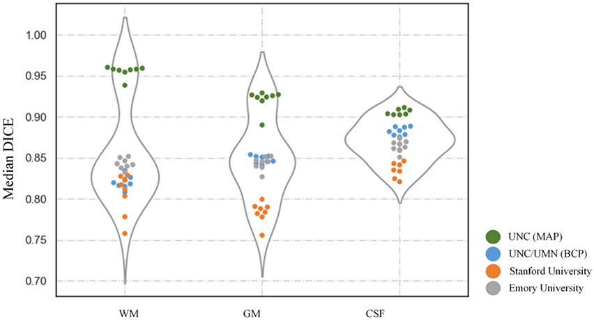
Based on the above evaluation and discussion, regarding the whole brain, ROIs, gyral curves and cortical thickness, we can conclude that unfortunately none of these 8 top-ranked methods can handle the multi-site issue well. The violin-plot shown in Fig. 17 illustrates the difference between validation and testing datasets. From Fig. 17, we can find there are two peaks in the violin-plots with regard to WM and GM, corresponding to the validation and testing datasets, which clearly indicates the critical problem caused by the multi-site issue. Moreover, all methods consistently perform poorly on Stanford University site, as median DICE values on Stanford University site are always at the bottom of each violin-plot. In addition, the Wilcoxon signed-rank tests among the validation dataset and three testing sites reported in Appendix Table VI also indicate that there is a statistically significant difference for GM on Stanford University site (p-value<0.05), compared with other testing sites. In the following, we will explore the origin of the multi-site issue, and why the performance on Stanford University site is always poor.

Fig. 17.

Average performance of 8 top-ranked methods on the validation dataset, and testing dataset (from three testing sites) based on median DICE for WM, GM, and CSF.

The multi-site issue is mainly caused by the “gap” between the training subjects and testing subjects. Many complicated factors could contribute to the “gap”, such as magnetic field, head coil, and TR/TE values. In the iSeg-2019 challenge, total 39 subjects of four sites were all acquired using 32-channel head coil and 3T scanners, therefore these two factors would less affect the difference of intensity distribution among the sites than the parameters of TR/TE, as listed in Table II. More specifically, the long TR minimizes T1w effects and short TE minimizes T2w effects [44], [45]. For example, the intensity I of an image can be estimated by

$$I=K\cdot [H]\cdot (1-e^{-TR∕T1})\cdot e^{-TE∕T2}$$

where K is a scaling factor and [H] is the spin (proton) density [44], [45]. When TE is made short compared to T2, the ratio TE/T2 → 0, thus the T2-weighted term e^−TE/T2→e⁻⁰ → 1. In other words, T2 effects largely disappear. It can be confirmed from Table II that for the T1w images, TE values across all sites (i.e., 4.4ms, 2.2ms, 2.9ms, 2.2ms) are consistently short. Similarly, when TR is made long compared to T1, the ratio TR/T1 → ∞, thus the T1-weighted term e^−TR/T1 → e^−∞ → 0. That is, T1 effects largely disappear. It can be confirmed from Table II that for the T2w images, TR values across all sites (i.e., 7380ms, 3200ms, 2502ms, 3200ms) are consistently long. Based on the above analysis, we could infer that the T1w (T2w) image is mainly affected by the parameter TR (TE). Therefore, in the following, we will mainly focus on TR values for T1w images and TE values for T2w images. From Table II, we can see that for the T1w images, the TR value of Stanford University site is significantly different from that of UNC (MAP), UNC/UMN (BCP), and Emory University sites, which is further confirmed from Fig. 2(a) that the T1w data distribution of Stanford University site (orange color) is different from other sites. For the T2w images, the UNC (MAP) and Stanford University sites share similar TE values, while UNC/UMN (BCP) and Emory University sites share another similar TE values. Accordingly, Fig. 2(b) also indicates that the UNC (MAP) and Stanford University sites share similar data distributions, while UNC/UMN (BCP) and Emory University sites share another similar data distribution. Overall, the Stanford University site exhibits different distribution in comparison of other sites, especially for the T1w images. The above analysis generally explains why most methods perform poorly on the testing subjects from Stanford University site. Based on our discussion on the origin of the multi-site issue in terms of imaging parameters, it might be worth investigating to map the images from the testing site to the space of training images based on MR imaging physics.

TABLE II.

TR/TE Values (in ms) of the iSeg-2019 Datasets

		Training /Validation	Testing
Site		UNC (MAP)	UNC/UMN (BCP)	Stanford University	Emory University
T1w	TR	1900	2400	7.6	2400
	TE	4.4	2.2	2.9	2.2
T2w	TR	7380	3200	2502	3200
	TE	119	564	91.4	561

First, although none of the teams can perform consistently across different sites, these teams with domain adaptation did achieve much better performance than these teams without domain adaptation (Figs. 12 and 16, and Appendix Tables II and XI), indicating that domain adaptation is a possible way to alleviate the multi-site issue. For example, QL111111 mimicked different intensity distributions by adjusting image contrast, to deal with the multi-site issue. xflz applied a tissue-dependent intensity augmentation method to simulate the variations in contrast. In order to decrease the distribution difference of multi-sites, CU_SIAT adopted EMNet to align distributions between training and testing datasets by using a discriminator network, and SmartDSP proposed Ada-nnUNet by utilizing a feature-level domain discriminator at the bottleneck layer of nnU-Net. Based on our discussion on the origin of the multi-site issue in terms of imaging parameters, it might be worth investigating to map the images from the testing site to the space of training images based on MR imaging physics.

Second, the prior knowledge of human brain, which is site-independent/scanner-independent, could be employed to guide the tissue segmentation. For example, cortical thickness, defined as the distance between the outer cortical surface (i.e., CSF and GM boundary) and inner cortical surface (i.e., GM and WM boundary), is within a certain range [25], [43]. Considering that CSF is relatively easier to be distinguished [25], [26], we could first identify the CSF from infant brain images. Then, based on the CSF segmentation and cortical thickness, we can estimate the outer cortical surface, and use it as guidance to locate the inner cortical surface. Our previous works have demonstrated the effectiveness of using the prior in helping the tissue segmentation [25], [26]. However, most of the participating teams only directly apply existing neural networks (e.g., U-Nets) to the multi-site subjects, without considering any site-independent/scanner-independent prior knowledge.

Third, the key highlights and implementation details of the 8 top-ranked methods are listed in Table III. For example, all methods randomly select 3D patches during the training stage, which could be improved by selecting more patches from the error-prone regions. As shown in Fig. 18, the main error regions exist in cortical regions, such as straight gyrus and lingual gyrus, therefore, more training patches from these error-prone regions may improve the segmentation performance. In addition, although training labels are always limited, we could employ a semi-supervised learning strategy or use existing methods to generate auxiliary labels [46] from the unlabeled testing subjects for better training.

Fig. 18.

The error map of all 8 top-ranked methods on testing subjects from three sites, i.e., UNC/UMN (BCP), Stanford University and Emory University. Color bar is from 0 to 1, with high values indicating large errors.

Finally, we would like to indicate limitations for the iSeg-2019. First, due to word count limitations, only 8 top-ranked methods were reviewed in this paper, but some other teams demonstrate useful strategies. For example, WorldSeg adopted a contour regression block to cope with the blurry boundary problem. SISE used 3D CycleGAN for domain adaptation between different sites. SJTU-IMR computed distance maps acquired by 3D U-Net to model the spatial context information, which can be viewed as one channel of FCN input to get the final segmentation. MASI applied the pertained model based on adult SLANT on the testing subjects. Second, the number of subjects is limited, e.g., only 5 or 6 subjects from each testing site, which may not well represent the multi-site issue. Third, only Siemens and GE scanners are included in this challenge. Fourth, 3T magnetic field adopted in the iSeg-2019 challenge is widely used in infant brain scanning, but it is also worthwhile to include 1.5T imaging data in future challenge. Fifth, the inter-rater variability is helpful to know the upper bound of the automated segmentation results; however, due to the huge amount of annotation work, in the iSeg-2019 challenge, the manual segmentation was performed by only one experienced expert, which is the biggest limitation of the challenge. We are going to solve this issue by employing multi-experts in the coming challenge. For our planned challenge, we will include more sites with various scanners/models, more testing subjects and employ multi-experts to further ensure the quality of manual annotations and measure the upper bound accuracy for the automated segmentation results.

VI. Conclusion

In this paper, we reviewed and summarized 30 automatic infant brain segmentation methods participated in the iSeg-2019 involving multi-site imaging data. We elaborated on the details of 8 top-ranked methods, including the pipeline, implementation, experimental results, and evaluations. We also discussed their limitations and possible future directions. In particular, we draw the following major conclusions:

1. The multi-site issue that learning-based models often perform poorly on testing subjects acquired with different imaging protocols/scanners as the training subjects, hinders the popularity and practicability of learning-based methods.

2. Although most participating methods employed advanced deep learning techniques, none of them can achieve consistent performance across different sites with different imaging protocols/scanners.

3. The multi-site issue is mainly caused by the different imaging protocols/scanners. It might be worth investigating to harmonize images from different sites based on MR imaging physics.

4. Domain adaptation is kind of helpful to alleviate the multi-site issue but does not fundamentally solve the issue.

5. It might be worth exploring the site-independent anatomy prior information to alleviate the multi-site issue.

The multi-site issue is still an open question and the iSeg-2019 website is always open. Although there are still some limitations in the iSeg-2019 challenge, we hope it may serve as a start point and attract researchers’ attention, as well as promote further methodological development for addressing the multi-site issue.

References

- [1].Wang L et al. , “Benchmark on automatic six-month-old infant brain segmentation algorithms: The iSeg-2017 challenge,” IEEE Trans. Med. Imag, vol. 38, no. 9, pp. 2219–2230, September. 2019. [DOI] [PMC free article] [PubMed] [Google Scholar]
- [2].Penny WD, Friston KJ, Ashburner JT, Kiebel SJ, and Nichols TE, Statistical Parametric Mapping: The Analysis of Functional Brain Images. Amsterdam, The Netherlands: Elsevier, 2011. [Google Scholar]
- [3].Ad-Dab’bagh Y et al. , “The CIVET image-processing environment: A fully automated comprehensive pipeline for anatomical neuroimaging research,” in Proc. 12th Annu. Meeting Org. Hum. Brain Mapping, Florence, Italy, 2006. [Google Scholar]
- [4].Shattuck D and Leahy R, “Brainsuite: An automated cortical surface identification tool,” Med. Image Anal, vol. 6, no. 2, pp. 129–142, 2002. [DOI] [PubMed] [Google Scholar]
- [5].Jenkinson M, Beckmann CF, Behrens TE, Woolrich MW, and Smith SM, “FSL,” NeuroImage, vol. 62, no. 2, pp. 782–790, 2012. [DOI] [PubMed] [Google Scholar]
- [6].Fischl B, “FreeSurfer,” NeuroImage, vol. 62, no. 2, pp. 774–781, August. 2012. [DOI] [PMC free article] [PubMed] [Google Scholar]
- [7].Glasser MF et al. , “The minimal preprocessing pipelines for the human connectome project,” NeuroImage, vol. 80, pp. 105–124, October. 2013. [DOI] [PMC free article] [PubMed] [Google Scholar]
- [8].Weisenfeld NI and Warfield SK, “Automatic segmentation of new-born brain MRI,” NeuroImage, vol. 47, no. 2, pp. 564–572, August. 2009. [DOI] [PMC free article] [PubMed] [Google Scholar]
- [9].Gui L, Lisowski R, Faundez T, Hüppi PS, Lazeyras FO, and Kocher M, “Morphology-driven automatic segmentation of MR images of the neonatal brain,” Med. Image Anal, vol. 16, no. 8, pp. 1565–1579, 2012. [DOI] [PubMed] [Google Scholar]
- [10].Hazlett HC et al. , “Brain volume findings in 6-month-old infants at high familial risk for autism,” Amer. J. Psychiatry, vol. 169, no. 6, pp. 601–608, 2012. [DOI] [PMC free article] [PubMed] [Google Scholar]
- [11].Paus T, Collins DL, Evans AC, Leonard G, Pike B, and Zijdenbos A, “Maturation of white matter in the human brain: A review of magnetic resonance studies,” Brain Res. Bull, vol. 54, no. 3, pp. 255–266, February. 2001. [DOI] [PubMed] [Google Scholar]
- [12].Makropoulos A et al. , “The developing human connectome project: A minimal processing pipeline for neonatal cortical surface reconstruction,” NeuroImage, vol. 173, pp. 88–112, July. 2018. [DOI] [PMC free article] [PubMed] [Google Scholar]
- [13].Zöllei L, Eugenio Iglesias J, Ou Y, Ellen Grant P, and Fischl B, “Infant FreeSurfer: An automated segmentation and surface extraction pipeline for T1-weighted neuroimaging data of infants 0–2 years,” 2020, arXiv:2001.03091 [Online]. Available: http://arxiv.org/abs/2001.03091 [DOI] [PMC free article] [PubMed] [Google Scholar]
- [14].Litjens G et al. , “Evaluation of prostate segmentation algorithms for MRI: The PROMISE12 challenge,” Med. Image Anal, vol. 18, no. 2, pp. 359–373, February. 2014. [DOI] [PMC free article] [PubMed] [Google Scholar]
- [15].Campello V et al. , “Multi-centre, multi-vendor and multi-disease cardiac segmentation: The M&Ms challenge,” IEEE Trans. Med. Imag., to be published [DOI] [PubMed] [Google Scholar]
- [16].Motiian S, Jones Q, Iranmanesh S, and Doretto G, “Few-shot adversarial domain adaptation,” in Proc. Adv. Neural Inf. Process. Syst, 2017, pp. 6670–6680. [Google Scholar]
- [17].Tzeng E, Hoffman J, Darrell T, and Saenko K, “Simultaneous deep transfer across domains and tasks,” in Proc. IEEE Int. Conf. Comput. Vis., December. 2015, pp. 4068–4076. [Google Scholar]
- [18].Sun Y et al. , “Semi-supervised transfer learning for infant cerebellum tissue segmentation,” in Proc. MLMI. Lima, Peru: Springer, 2020, pp. 663–673. [DOI] [PMC free article] [PubMed] [Google Scholar]
- [19].Sun B, Feng J, and Saenko K, “Return of frustratingly easy domain adaptation,” in Proc. 13th AAAI Conf. Artif. Intell., 2016, pp. 2058–2065. [Google Scholar]
- [20].Tzeng E, Hoffman J, Saenko K, and Darrell T, “Adversarial discriminative domain adaptation,” in Proc. IEEE Conf. Comput. Vis. Pattern Recognit. (CVPR), July. 2017, pp. 7167–7176. [Google Scholar]
- [21].Yin W, Chen M-H, Hung S-C, Baluyot KR, Li T, and Lin W, “Brain functional development separates into three distinct time periods in the first two years of life,” NeuroImage, vol. 189, pp. 715–726, April. 2019. [DOI] [PubMed] [Google Scholar]
- [22].Shi F, Wang L, Dai Y, Gilmore JH, Lin W, and Shen D, “LABEL: Pediatric brain extraction using learning-based meta-algorithm,” NeuroImage, vol. 62, no. 3, pp. 1975–1986, September. 2012. [DOI] [PMC free article] [PubMed] [Google Scholar]
- [23].Sled JG, Zijdenbos AP, and Evans AC, “A nonparametric method for automatic correction of intensity nonuniformity in MRI data,” IEEE Trans. Med. Imag, vol. 17, no. 1, pp. 87–97, February. 1998. [DOI] [PubMed] [Google Scholar]
- [24].Wang L, Shi F, Yap P-T, Lin W, Gilmore JH, and Shen D, “Longitudinally guided level sets for consistent tissue segmentation of neonates,” Hum. Brain Mapping, vol. 34, no. 4, pp. 956–972, April. 2013. [DOI] [PMC free article] [PubMed] [Google Scholar]
- [25].Wang L et al. , “Volume-based analysis of 6-month-old infant brain MRI for autism biomarker identification and early diagnosis,” in Proc. MICCAI, vol. 11072. Granada, Spain: MICCAI, 2018, pp. 411–419. [DOI] [PMC free article] [PubMed] [Google Scholar]
- [26].Wang L et al. , “Anatomy-guided joint tissue segmentation and topological correction for 6-month infant brain MRI with risk of autism,” Hum. Brain Mapping, vol. 39, no. 6, pp. 2609–2623, 2018. [DOI] [PMC free article] [PubMed] [Google Scholar]
- [27].Zhang K and Sejnowski TJ, “A universal scaling law between gray matter and white matter of cerebral cortex,” Proc. Nat. Acad. Sci. USA, vol. 97, no. 10, pp. 5621–5626, May 2000. [DOI] [PMC free article] [PubMed] [Google Scholar]
- [28].Lei Z, Qi L, Wei Y, Zhou Y, and Zhang Y. Infant Brain MRI Segmentation With Dilated Convolution Pyramid Downsampling and Self-Attention. Accessed: Dec. 1, 2019. [Online]. Available: https://ui.adsabs.harvard.edu/abs/2019arXiv191212570L
- [29].Pohlen T, Hermans A, Mathias M, and Leibe B, “Full-resolution residual networks for semantic segmentation in street scenes,” in Proc. IEEE Conf. Comput. Vis. Pattern Recognit., July. 2017, pp. 4151–4160. [Google Scholar]
- [30].Woo S, Park J, Lee J-Y, and So Kweon I, “CBAM: Convolutional block attention module,” in Proc. Eur. Conf. Comput. Vis., 2018, pp. 3–19. [Google Scholar]
- [31].Çiçek Ö, Abdulkadir A, Lienkamp SS, Brox T, and Ronneberger O, “3D U-Net: Learning dense volumetric segmentation from sparse annotation,” in Proc. MICCAI. Athens, Greece: Springer, 2016, pp. 424–432. [Google Scholar]
- [32].Isensee F, Jäger PF, Kohl SAA, Petersen J, and Maier-Hein KH, “Automated design of deep learning methods for biomedical image segmentation,” 2019, arXiv:1904.08128 [Online]. Available: http://arxiv.org/abs/1904.08128 [Google Scholar]
- [33].Dou Q, Ouyang C, Chen C, Chen H, and Heng P-A, “Unsupervised cross-modality domain adaptation of ConvNets for biomedical image segmentations with adversarial loss,” in Proc. 27th Int. Joint Conf. Artif. Intell., July. 2018, pp. 691–697. [Google Scholar]
- [34].Saito K, Ushiku Y, Harada T, and Saenko K, “Strong-weak distribution alignment for adaptive object detection,” in Proc. IEEE/CVF Conf. Comput. Vis. Pattern Recognit. (CVPR), June. 2019, pp. 6956–6965. [Google Scholar]
- [35].Bui TD, Shin J, and Moon T, “Skip-connected 3D DenseNet for volumetric infant brain MRI segmentation,” Biomed. Signal Process. Control, vol. 54, September. 2019, p. 101613. [Google Scholar]
- [36].Pan X, Luo P, Shi J, and Tang X, “Two at once: Enhancing learning and generalization capacities via IBN-Net,” in Proc. Eur. Conf. Comput. Vis., 2018, pp. 464–479. [Google Scholar]
- [37].Vu T-H, Jain H, Bucher M, Cord M, and Pérez P, “Advent: Adversarial entropy minimization for domain adaptation in semantic segmentation,” in Proc. IEEE Conf. Comput. Vis. Pattern Recognit., June. 2019, pp. 2517–2526. [Google Scholar]
- [38].Roy AG, Navab N, and Wachinger C, “Concurrent spatial and channel ‘squeeze & excitation’ in fully convolutional networks,” in Proc. MICCAI. Madrid, Spain: Springer, 2018, pp. 421–429. [Google Scholar]
- [39].Dolz J, Gopinath K, Yuan J, Lombaert H, Desrosiers C, and Ben Ayed I, “HyperDense-net: A hyper-densely connected CNN for multi-modal image segmentation,” IEEE Trans. Med. Imag, vol. 38, no. 5, pp. 1116–1126, May 2019. [DOI] [PubMed] [Google Scholar]
- [40].Srivastava N, Hinton G, Krizhevsky A, Sutskever I, and Salakhutdinov R, “Dropout: A simple way to prevent neural networks from overfitting,” J. Mach. Learn. Res, vol. 15, no. 1, pp. 1929–1958, 2014. [Google Scholar]
- [41].Avants BB, Tustison NJ, Song G, Cook PA, Klein A, and Gee JC, “A reproducible evaluation of ANTs similarity metric performance in brain image registration,” NeuroImage, vol. 54, no. 3, pp. 2033–2044, February. 2011. [DOI] [PMC free article] [PubMed] [Google Scholar]
- [42].Barkovich AJ, Guerrini R, Kuzniecky RI, Jackson GD, and Dobyns WB, “A developmental and genetic classification for malformations of cortical development: Update 2012,” Brain, vol. 135, no. 5, pp. 1348–1369, May 2012. [DOI] [PMC free article] [PubMed] [Google Scholar]
- [43].Li G et al. , “Measuring the dynamic longitudinal cortex development in infants by reconstruction of temporally consistent cortical surfaces,” NeuroImage, vol. 90, pp. 266–279, April. 2014. [DOI] [PMC free article] [PubMed] [Google Scholar]
- [44].Plewes DB, “The AAPM/RSNA physics tutorial for residents. Contrast mechanisms in spin-echo MR imaging,” Radiographics, vol. 14, no. 6, pp. 1389–1404, 1994. [DOI] [PubMed] [Google Scholar]
- [45].Perman W, Hilal S, Simon H, and Maudsley A, “Contrast manipulation in NMR imaging,” Magn. Reson. Imag, vol. 2, no. 1, pp. 23–32, 1984. [DOI] [PubMed] [Google Scholar]
- [46].Huo Y et al. , “3D whole brain segmentation using spatially localized atlas network tiles,” NeuroImage, vol. 194, pp. 105–119, July. 2019. [DOI] [PMC free article] [PubMed] [Google Scholar]
Associated Data
This section collects any data citations, data availability statements, or supplementary materials included in this article.