Concurrent assessment of personal, indoor, and outdoor PM_2.5 and PM₁ levels and source contributions using novel low‐cost sensing devices

Abstract

The intensity, frequency, duration, and contribution of distinct PM_2.5 sources in Asian households have seldom been assessed; these are evaluated in this work with concurrent personal, indoor, and outdoor PM_2.5 and PM₁ monitoring using novel low‐cost sensing (LCS) devices, AS‐LUNG. GRIMM‐comparable observations were acquired by the corrected AS‐LUNG readings, with R ² up to 0.998. Twenty‐six non‐smoking healthy adults were recruited in Taiwan in 2018 for 7‐day personal, home indoor, and home outdoor PM monitoring. The results showed 5‐min PM_2.5 and PM₁ exposures of 11.2 ± 10.9 and 10.5 ± 9.8 µg/m³, respectively. Cooking occurred most frequently; cooking with and without solid fuel contributed to high PM_2.5 increments of 76.5 and 183.8 µg/m³ (1 min), respectively. Incense burning had the highest mean PM_2.5 indoor/outdoor (1.44 ± 1.44) ratios at home and on average the highest 5‐min PM_2.5 increments (15.0 µg/m³) to indoor levels, among all single sources. Certain events accounted for 14.0%‐39.6% of subjects’ daily exposures. With the high resolution of AS‐LUNG data and detailed time‐activity diaries, the impacts of sources and ventilations were assessed in detail.

Practical Implications.

• This is the first work demonstrating the applicability of low‐cost sensing (LCS) devices in concurrent personal, indoor, and outdoor PM assessment.

• One personal LCS device, AS‐LUNG‐P, with high time resolution can detect peak PM_2.5 and PM₁ exposures.

• LCS devices, AS‐LUNG‐I and AS‐LUNG‐O, are suitable for home indoor and outdoor PM_2.5 and PM₁ assessment, respectively.

• LCS devices identified important indoor exposure sources and quantified their contributions.

• This work shows great potential of LCS devices in future PM studies and citizen science.

1. INTRODUCTION

Household air pollution is one of the leading environmental risk factors for death with particulate matter with an aerodynamic diameter less than or equal to 2.5 μm (PM_2.5), a classified human carcinogen, ¹ as a major concern. ² , ³ , ⁴ In particular, Asia accounted for two‐thirds of global premature deaths, with 1.64 million in 2017 due to household air pollution, ³ , ⁴ while the intensities, frequencies, durations, and contribution of distinct PM_2.5 sources in Asian households have seldom been evaluated. In addition, indoor infiltration of high ambient PM_2.5 levels in Asia ⁵ affecting Indoor Air Quality (IAQ) exacerbates exposure levels indoors. Characterizing PM_2.5 exposures due to these sources in Asian households is critical for both environmental health research and health advisories to reduce the associated health risks. ⁶ , ⁷

PM_2.5 exposures are usually higher than the ambient levels measured by regulatory monitoring stations. ⁷ , ⁸ , ⁹ Distinct sources in Asian households such as cooking and incense burning generate high PM_2.5 emissions, ¹⁰ , ¹¹ leading to peak exposures that may trigger acute health effects. Using outdoor ambient PM_2.5 levels as coarsely estimated PM_2.5 exposure surrogates, like most previous studies, faces the challenge of underestimating exposure levels and health damages. ¹² Recent advances in low‐cost sensing (LCS) devices enable an accurate assessment of PM_2.5 exposure ¹³ and sources in indoor environments where people spend most of their time. ¹⁴ The current work takes advantage of LCS devices in characterizing indoor exposure to facilitate the formulation of effective behavior change recommendations and source reduction strategies for health risk reductions.

PM_2.5 exposures were traditionally assessed using personal samplers with integrated filter samples or expensive real‐time personal monitors. ⁸ , ¹⁵ , ¹⁶ The noise, vibration, and conspicuous appearance of samplers with a pump or real‐time monitors have often discouraged subjects from adhering to their daily routines when carrying samplers/monitors. Exposure sources associated with physical activities are less likely to be identified and evaluated if subjects change their behaviors on monitoring days. The newly developed small and lightweight LCS devices overcome these drawbacks and allow subjects to move freely, thus enabling closer‐to‐reality PM_2.5 exposure assessment.

LCS devices integrate low‐cost sensors, data transmission/storage, and power supply components. ¹⁷ Application of LCS devices may shift the paradigm of personal exposure assessment and IAQ research ¹⁸ , ¹⁹ after the challenge of data quality issues is tackled. ²⁰ Several PM_2.5 sensors have been evaluated against research‐grade instruments such as GRIMM, SidePak, and the tapered element oscillating microbalance (TEOM) analyzer. ¹⁷ , ²¹ , ²² PMS3003 was chosen in this work based on our previous evaluation showing that the R ² between PMS3003 and GRIMM was as high as 0.9825 for PM₁ and 0.9843 for PM_2.5. ¹⁷ The objective of this work was to assess the intensity, frequency, duration, and contribution of PM sources, especially in Asian households, with concurrent personal, indoor, and outdoor GRIMM‐comparable PM_2.5 and PM₁ measurements converted from LCS‐device readings. The influence of ventilation on PM levels was also evaluated. The lessons learned can shed light on the application of LCS devices to exposure assessment and IAQ evaluation.

2. MATERIALS AND METHODS

2.1. AS‐LUNG sets

With modification from a prototype, ¹⁷ three versions of LCS devices, namely AS‐LUNG‐P, AS‐LUNG‐I, and AS‐LUNG‐O, were integrated with PMS3003 (Plantower, Beijing, China) by our team for different purposes. AS stands for Academia Sinica, the research institute supporting its development; LUNG indicates the human organ most affected by air pollutants; P, I, and O stand for portable, indoor, and outdoor, respectively. PMS3003 uses a laser light source with 90° scattered light detected by a photo‐diode detector. ²³ While it is ineffective in detecting PM_2.5‐10, ²⁴ its volume‐scattering detection approach can obtain PM_2.5 measurements independent of the flow rate. ²⁵ Moreover, its reported mean time to failure is more than three years, ²⁶ consistent with our experience. PMS3003 also provided stable readings in field evaluations in Taiwan with high relative humidity (RH%, 74 ± 11%). ²⁷ Furthermore, as discussed previously, ²⁷ our work is health‐oriented research not aiming for regulatory purposes that determine areas not compliant with the air quality standards requiring PM measured in certain temperature and humidity ranges. This study aimed to assess the PM that is actually being inhaled, including water droplets ≤2.5 μm suspended in the air. Hence, PMS3003 with the light‐scattering principle was chosen, as it measures PM without artificially controlling for humidity. Although it is not the newest Plantower sensor, its precision, stability, and long lifetime make it a useful tool for research.

AS‐LUNG‐I (Figure 1), with a basic manufacturing cost of 240 USD, without considering research and development costs, was used for indoor monitoring. Sensors for PM (PMS3003), CO₂ (S8, Senseair AB, Sweden), temperature/humidity (SHT31, Sensirion AG, Switzerland), motion (ADXL345B, Analog Devices, Inc, USA), and real‐time clock module are integrated within the device of 140 × 100 × 40 mm in size and 208 g in weight. The outer case is not entirely enclosed to avoid heat buildup, with a screen displaying real‐time observations in Chinese and English (Figure S1). Real‐time data are transmitted wirelessly with the built‐in Wi‐Fi module through a 4G router back to the cloud database at one of the three log intervals, namely 15 seconds, 1 minute, and 5 minutes. A complementary SD card is added to avoid data loss. Power can be supplied from an electric socket or a mobile battery. This small device without noise and vibration can be easily deployed in various indoor environments without disturbing those present.

FIGURE 1.

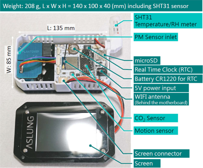
Low‐cost PM sensing device, AS‐LUNG‐I, with various components marked

The design of the AS‐LUNG‐P (270 USD), adapted for exposure assessment, has been described earlier. ¹³ In brief, it has the same set of sensors as AS‐LUNG‐I, plus a GPS, with several minor differences. Designed to be portable, AS‐LUNG‐P has a smaller display screen, 135 × 70 × 40 mm in size, and is lighter, 153 g in weight (Figures S2 and S3). When being carried around, a mobile battery is its power source; otherwise, it can be charged at an electric socket. AS‐LUNG‐P has a different outer case, mostly enclosed except for openings of sensors, the SD card, and plugs.

AS‐LUNG‐O (650 USD) was used for outdoor monitoring with the same sets of sensors. The design and its application to community source evaluation have been presented earlier. ²⁷ Briefly, its sensors are placed in a waterproof shelter connected to a solar panel and backup batteries for power supply, with the option of using household electricity when easily accessible. This device can be easily set up in the patios or balconies outside residences.

To ensure data quality, each AS‐LUNG underwent a side‐by‐side comparison in laboratory against a GRIMM (GRIMM 1.109, GRIMM Aerosol Technik Ainring GmbH & Co, Ainring, Germany) with procedures described earlier. ²⁷ , ²⁸ In short, correction equations were established using data from collocated AS‐LUNG and GRIMM during the concentration decay period (well‐mixed) after incense burning inside an almost closed hood. GRIMM is a spectrometer detecting aerosols in the size range of 0.25‐32 μm in 31 size channels, with a similar laser wavelength (655 nm) to that of PMS3003 (655 ± 10 nm). ²³ The data of GRIMM agree well with those of an EDM‐180 (R ² = 0.9997), a federal equivalent method (FEM) instrument designated by USEPA for PM_2.5 with the same light‐scattering principle. ²⁸

Readings of each AS‐LUNG were converted by the respective correction equations obtained in the laboratory into GRIMM‐comparable measurements. The linear range of these correction curves could be up to 400‐500 µg/m³. To reduce conversion errors in lower ranges, this work used correction equations up to 150 µg/m³, which covers the majority of environmental PM_2.5 levels in Taiwan. The slopes and R ² of the correction equations of these LCS devices are listed in Table S1. High R ² (mostly 0.895‐0.998) indicated that AS‐LUNG sets are qualified to be used in PM_2.5 and PM₁ research, after data correction.

2.2. Subject recruitment and monitoring strategies

Twenty‐six non‐smoking subjects (9 males and 17 females) aged 40‐75 years without pre‐existing cardiovascular diseases were recruited from a community in New Taipei City, Taiwan. Their households were all located within a circle with a radius of 500 m. Written informed consent was obtained from all subjects before the field campaign. Each subject was required to carry one AS‐LUNG‐P (15‐seconds resolution) for 7 days in September and October 2018. AS‐LUNG‐P could be worn near the chest, strapped around the waist, or carried in a bag with the inlet protruding. Subjects were asked to keep their daily routines as usual. During shower and sleep, AS‐LUNG‐P was to be placed outside the bathroom and at the bedside, respectively. Concurrently, one AS‐LUNG‐I (15‐sec resolution) was set up in the household living room with one AS‐LUNG‐O (1‐min resolution) in the immediate outdoor environment (such as balcony or sidewalk) to assess home indoor and outdoor PM levels, respectively.

Before monitoring commenced, demographic data of the subjects and the details of their habits and potential exposure sources were solicited in a face‐to‐face interview with a questionnaire. During monitoring, subjects had to fill out a time‐activity diary (TAD) at 30‐min intervals regarding their microenvironments, activities, ventilation status if indoors, and major exposure sources encountered. The exposure source question probes into nearby sources, rather than distant sources such as industrial parks (unless there was a clear indication that subjects were exposed to pollution from distant sources, such as visible fires). Confirmation with each subject was performed to ensure the validity and completeness of TAD records, which were utilized to identify and assess high‐exposure sources and microenvironments. The study design was approved by the Institutional Review Board of Academia Sinica (AS‐IRB‐BM‐18053).

2.3. Data analysis

After excluding data during raining hours, only those available for all three categories (personal, indoor, and outdoor) were kept in the dataset and converted into GRIMM‐comparable observations using correction equations obtained in the laboratory. Owing to conversion errors, 9.05% of PM₁ levels were slightly higher than PM_2.5 after conversions and thus substituted by PM_2.5. Further analysis for exposure sources focused on PM_2.5 only because they were likely from the same sources, as evidenced in the Results section.

Five‐minute averages were used in the subsequent data analysis, with the exception of 1‐min peak exposures used in case evaluations. Ratios of indoor to outdoor (I/O), of personal to indoor (P/I), and of personal to outdoor (P/O) levels were calculated using 5‐min concurrent measurements. Measurements under different classifications were compared using the Wilcoxon rank‐sum test or the Kruskal‐Wallis test plus the Dunn test. Correlations between different measurements were assessed with Spearman's rank correlation coefficients (r_s), while paired differences between concurrent measurements were evaluated using the Wilcoxon sign‐ranked test.

Source contributions to PM_2.5 were assessed by matching PM_2.5 with TAD records. Cases with interesting sources were plotted with personal, indoor, and outdoor levels. Mean PM_2.5 levels at one hour before these source emissions were taken as baselines for comparison with peaks (the maximum 1‐min observations) during source emissions. The difference between baselines and peaks was “the maximum PM_2.5 increment (µg/m³)” due to sources. Moreover, “PM_2.5 exposure summation (µg/m³‐h)” attributed to an event can be estimated with the total exposure duration multiplied by mean PM_2.5 level during the event. The event contribution (%) was calculated as the percentage of PM_2.5 exposure summation of that event accounting for the daily (midnight to 11:59 PM) PM_2.5 exposure summation of that subject.

Multiple regression was applied to evaluate important factors of personal PM_2.5 exposures and indoor PM_2.5 concentrations as in Models (1‐3):

$${\mathrm{PM}}_{\mathrm{personal}}={\alpha }_0+{\mathrm{\gamma }}_1{\mathrm{PM}}_{\mathrm{indoor}}+{\mathrm{\gamma }}_2{\mathrm{PM}}_{\mathrm{outdoor}}$$ (1)

$${\mathrm{PM}}_{\mathrm{personal}}={\alpha }_0\text{+}\sum \beta iXi+{\mathrm{\gamma }}_2{\mathrm{PM}}_{\mathrm{outdoor}}+\sum \mathrm{\zeta }iVi$$ (2)

$${\mathrm{PM}}_{\mathrm{indoor}}={\alpha }_0\text{+}\sum \beta iXi+{\mathrm{\gamma }}_2{\mathrm{PM}}_{\mathrm{outdoor}}+\sum \mathrm{\zeta }iVi$$ (3)

where PM_personal, PM_indoor, and PM_outdoor are personal, indoor, and outdoor PM_2.5 levels, respectively; ${\alpha }_0$ is the intercept; and βi is the regression coefficient of Xi, which is a dummy variable representing different sources recorded in TADs, with no recorded source as the base case. Sources encountered less than 100 times (sample size of the total valid 30‐min records of 26 subjects is 9350) were not incorporated into the model in order to focus on significant ones. ${\gamma }_1$ and ${\gamma }_2$ are regression coefficients of indoor and outdoor PM_2.5 levels, respectively. ζi is the regression coefficient of Vi, a dummy variable of ventilation statuses. Typical ventilation statuses in the households included windows open without air conditioning (AC) (hereinafter window‐open, the base case), windows closed without AC (hereinafter window‐closed), and windows closed with AC on (hereinafter AC‐on). Three models were established with stepwise regression for the periods of the subjects at home (hereinafter at‐home period). Model 1 assessed the explanation power of indoor and outdoor levels for PM_2.5 personal exposures. Model 2 assessed the relationship of PM_2.5 exposures with outdoor levels plus source and ventilation terms. Model 3 assessed the relationship of indoor PM_2.5 with outdoor PM_2.5 levels, various indoor sources, and ventilation status.

3. RESULTS

During the 182 person‐day monitoring campaign, the data collection rates for AS‐LUNG‐P, AS‐LUNG‐I, and AS‐LUNG‐O were 94.4%, 96.5%, and 96.4%, respectively. Data loss was due to electricity shutdowns at households or battery compatibility issues, which were solved during the field campaign. No ghost peaks or negative signals were observed.

The sample size for all three categories (personal, indoor, and outdoor) was 37 963 (5‐minutes observations) in the 182 person‐day monitoring after excluding raining hours. Of 5‐minutes personal, indoor, and outdoor PM_2.5 averages, there were 47, 65, and 7 measurements greater than 150 µg/m³, accounting for 0.12%, 0.17%, and 0.02% of the total measurements, respectively, with even smaller numbers for PM₁. Greater conversion errors would occur in data above 150 µg/m³. These high PM levels were still included in the dataset because an essential purpose of exposure assessment is to evaluate peaks.

3.1. PM_2.5 and PM₁ levels

Table 1 shows PM_2.5 and PM₁ levels for different classifications. As can be seen, mean personal, indoor, and outdoor levels for PM_2.5 in the entire non‐raining period were 11.2 ± 10.9, 14.8 ± 13.8, and 18.4 ± 10.6 µg/m³, respectively. Those for PM₁ were 10.5 ± 9.8, 14.0 ± 12.7, and 16.1 ± 7.9 µg/m³, respectively. The maximum of PM_2.5 (277.3 µg/m³) and PM₁ (201.0 µg/m³) occurred at home indoors when the subjects burned incenses and joss papers (Table 1A). For comparisons, PM_2.5 and PM₁ personal, home indoor, and home outdoor levels were statistically significantly higher at daytime (8am‐8pm) than at nighttime, presumably due to PM‐generation human activities at daytime. Similar PM₁ and PM_2.5 levels were observed in all categories, with high PM₁/PM_2.5 ratios of 0.94 ± 0.05 for personal exposure, 0.94 ± 0.05 for home indoor, and 0.89 ± 0.09 for home outdoor levels, indicating that direct PM_2.5 exposures were mainly from PM₁‐generating sources, most likely combustion sources. For microenvironments, subjects staying outdoors had higher PM_2.5 and PM₁ exposures than those indoors (Table 1B). In indoor microenvironments, PM_2.5 and PM₁ exposures were the highest with window‐open, followed by window‐closed, and the lowest with AC‐on.

TABLE 1.

PM_2.5 and PM₁ concentrations (5 min, μg/m³) (A) with personal, home indoor, and home outdoor measurements for the entire non‐raining period, (B) for personal exposures in microenvironments with different classifications, and (C) with concurrent personal, home indoor, and home outdoor measurements for at‐home periods

(A) Entire non‐raining period	n	PM2.5			PM1
		Mean ± SD	Median	Maximum	Mean ± SD	Median	Maximum
Personal exposures	37 963	11.2 ± 10.9	9.1	207.6	10.5 ± 9.8	8.8	155.0
Home indoor levels	37 963	14.8 ± 13.8	12.5	277.3	14.0 ± 12.7	12.0	201.0
Home outdoor levels	37 963	18.4 ± 10.6	16.6	276.6	16.1 ± 7.9	14.9	193.5
Personal, daytime (8am‐8pm)	19 302	12.0 ± 11.9	9.8*	207.6	11.2 ± 10.5	9.4*	155.0
Nighttime (8am‐8pm)	18 661	10.3 ± 9.6	8.5	196.5	9.7 ± 8.5	8.3	134.7
Home indoor, daytime	19 302	16.2 ± 16.5	13.6*	277.3	15.3 ± 15.1	13.0*	201.0
Nighttime	18 661	13.4 ± 10.2	11.8	201.0	12.6 ± 9.5	11.4	157.7
Home outdoor, daytime	19 302	18.7 ± 10.8	16.7*	254.0	16.4 ± 8.1	15.2*	151.8
Nighttime	18 661	18.1 ± 10.3	16.4	276.6	15.7 ± 7.6	14.7	193.5

(B) Personal exposures (entire non‐raining period)	n	Personal PM2.5 exposures			Personal PM1 exposures
		Mean ± SD	Median	Maximum	Mean ± SD	Median	Maximum
Outdoor microenvironment	3311	12.8 ± 9.9	11.1*	126.9	11.9 ± 9.0	10.5*	112.9
Indoor microenvironment	34 652	11.0 ± 11.0	8.9	207.6	10.3 ± 9.7	8.7	155.0
Indoor with window‐open	24 240	11.5 ± 10.5	9.6*	207.6	10.8 ± 9.2	9.3*	155.0
Indoor with window‐closed	3953	10.4 ± 8.3	8.8	112.2	9.7 ± 8.1	8.6	112.2
Indoor with AC‐on	6459	9.6 ± 13.7	6.2	196.5	8.9 ± 11.8	5.9	134.7

(C) At‐home period	n	PM2.5			PM1
		Mean ± SD	Median	Maximum	Mean ± SD	Median	Maximum
Personal, daytime (8am‐8pm)	9433	13.5 ± 14.3	10.6*	207.6	12.6 ± 12.5	10.2*	155.0
Nighttime (8am‐8pm)	16 888	9.6 ± 7.0	8.3	139.6	9.1 ± 6.4	8.1	117.5
Home indoor, daytime	9433	17.2 ± 19.4	13.6*	277.3	16.2 ± 17.4	13.0*	201.0
Nighttime	16 888	13.1 ± 9.9	11.5	201.0	12.3 ± 9.1	11.4	157.7
Home outdoor, daytime	9433	19.0 ± 11.5	16.8*	254.0	16.6 ± 8.4	15.3*	151.8
Nighttime	16 888	17.9 ± 10.3	16.2	276.6	15.4 ± 7.6	14.5	193.5

Comparisons were all significant at p‐value < .001, marked with *. Comparisons were conducted between daytime and nighttime for (A) and (C) and among different aforementioned microenvironments for (B). Additionally, paired comparisons were conducted for PM_2.5 and PM₁ among personal exposure, the corresponding home indoor, and the corresponding home outdoor levels in (C).

Abbreviations: n, number of the 5‐min observations; SD, standard deviation.

According to TADs, these subjects spent 91.6 ± 4.2% and 70.2 ± 13.7% of their time indoors and at home, respectively. There were 11 subjects either working at home or acting as housewives; thus, the percentages of time spent at home were high. Therefore, the means and standard deviations of PM_2.5 and PM₁ for the at‐home period were further calculated and are presented in Table 1C (sample size of 5‐min observation is 26 321). The daytime PM levels continued to be higher than those at nighttime for the at‐home period. Additionally, personal PM_2.5 and PM₁ exposures were statistically significantly lower than the corresponding indoor levels, and they both in turn were statistically significantly lower than the corresponding outdoor levels (Table 1C).

In addition, for the entire non‐raining periods, among correlations of personal, indoor, outdoor, and their ratios for PM_2.5 and PM₁, correlations of personal vs. indoor and indoor vs. outdoor (r_s = 0.74‐0.78) were higher than those of personal vs. outdoor (r_s = 0.64‐0.66) (Table S2). During at‐home periods, correlations of personal exposure and indoor levels for PM_2.5 and PM₁ were the highest (0.81 and 0.83, respectively, Table S2). Considering the high correlations, the high percentage of time spent at home, and the unprecedentedly concurrent personal/indoor/outdoor measurements at home with LCS devices, the following results are focused on at‐home periods to assess indoor exposure events and sources at home.

During at‐home periods, mean I/O, P/I, and P/O ratios were 0.87, 0.79, and 0.66 for PM_2.5, with medians of 0.75, 0.76, and 0.57, respectively, slightly lower than those of PM₁ (Table 2). Considering building shielding effects, I/O and P/O ratios above 1 would indicate the occurrence of indoor exposure events, while these ratios in fact were mostly less than 1, suggesting that the subjects were not exposed to indoor sources most of the time. P/I mostly less than 1 showed that the subjects (with AS‐LUNG‐P) were possibly away from the sources than the AS‐LUNG‐I sets in the living rooms. For further evaluation, P/I ratios during sleep (the periods without nearby sources) were calculated. The median P/I ratios reduced even further to 0.73 and 0.74 for PM_2.5 and PM₁, respectively, showing that the subjects in the bedrooms were exposed to lower PM compared with the living rooms. When sleeping with AC‐on, the median P/I ratios of PM_2.5 and PM₁ were down to only 0.47 and 0.45, respectively, demonstrating PM reduction by AC (with certain filtering functions) in the bedrooms. Moreover, I/O ratios of PM_2.5 and PM₁ had higher means and standard deviations than P/I and P/O ratios in different classifications in Table 2; they are explored further with exposure sources recorded in TADs in the next section.

TABLE 2.

Ratios of indoor to outdoor (I/O), of personal to indoor (P/I), and of personal to outdoor (P/O) for (A) PM_2.5 and (B) PM₁ for at‐home periods

(A) PM2.5	At‐home periods		Sleep time (n = 11 019)		Sleep with AC‐on (n = 1116)
	PM2.5		PM2.5		PM2.5
	Mean (SD)	Median	Mean (SD)	Median	Mean (SD)	Median
I/O	0.87 (0.82)	0.75	0.78 (0.65)	0.69	0.82 (0.40)	0.78
P/I	0.79 (0.27)	0.76	0.76 (0.24)	0.73	0.51 (0.24)	0.47
P/O	0.66 (0.59)	0.57	0.56 (0.41)	0.51	0.42 (0.31)	0.28

(B) PM1	At‐home periods		Sleep time (n = 11 019)		Sleep with AC‐on (n = 1116)
	PM1		PM1		PM1
	Mean (SD)	Median	Mean (SD)	Median	Mean (SD)	Median
I/O	0.91 (0.80)	0.77	0.82 (0.61)	0.74	0.84 (0.41)	0.77
P/I	0.79 (0.24)	0.78	0.76 (0.21)	0.74	0.50 (0.25)	0.45
P/O	0.69 (0.57)	0.60	0.60 (0.40)	0.55	0.44 (0.33)	0.29

Moreover, air cleaners are another known factor of indoor PM_2.5 levels. Air cleaners are popular in high‐income families but not in ordinary households in Taiwan; thus, “owning an air cleaner” was in the questionnaire but “air cleaner usage” was not included in the TADs since there were already a lot of items to be recorded. Therefore, we only had information on whether the household owned an air cleaner but not on whether the subjects turned them on. In the face‐to‐face interview, 15 subjects indicated that they owned air cleaners at home. However, the lack of information of whether these air cleaners were turned on restrained us from further evaluation. Nevertheless, households with air cleaners had higher PM_2.5 and PM₁ levels than those without air cleaners (Table S3) under similar ambient PM_2.5 and PM₁ levels in the same community, implying minimum interference from air cleaners in this work (either not turned on or not effective enough in making significant impacts). Indoor events with subjects exposed to different sources at home indicated in the TADs were counted, and the results showed that the subjects at households with air cleaners had higher numbers of indoor events with sources (30‐min resolution, n = 339) compared to those households without air cleaners (n = 246). This may explain why the households with air cleaners had higher PM_2.5 and PM₁ levels indoors.

3.2. Intensity, frequency, and duration of indoor exposures from various sources

With the high‐resolution personal/indoor/outdoor levels and the detailed TAD records, the intensity, frequency, and durations of household exposure events were evaluated with different sources. Table 3A shows the 5‐min personal PM_2.5 exposures and the PM₁/PM_2.5 as well as the PM_2.5 I/O, P/I, and P/O ratios for the at‐home periods with different sources. For exposure sources, “incense burning” (n = 513) comprises data of both incense burning (n = 500) and joss paper burning (n = 12 plus one with both sources) since they are part of the traditional worshipping practices sometimes occurring simultaneously or successively. Other sources included scented candle burning, garbage odors, cleaning, mosquito coil burning, factories, and agriculture waste burning. Subjects may have encountered more than one source that was not classified or explored further.

TABLE 3.

For at‐home periods, (A) the 5‐min personal PM_2.5, the PM₁/PM_2.5, PM_2.5 indoor‐to‐outdoor (I/O), personal‐to‐indoor (P/I), and personal‐to‐outdoor (P/O) ratios with different sources, and (B) the 5‐min indoor PM_2.5 and PM_2.5 I/O ratios of indoor events with different sources and durations

(A)	Personal PM2.5 (μg/m3)			PM1/PM2.5	I/O ratios	P/I ratios	P/O ratios
	n	Mean (SD)	Median	Mean (SD)	Mean (SD)	Mean (SD)	Mean (SD)
Exposure sources
Cooking	1685	14.9 (16.0)	12.0	0.92 (0.06)	0.86 (0.77)	0.91 (0.33)	0.73 (0.63)
Environmental tobacco smoke	334	15.2 (10.6)	11.7	0.96 (0.02)	0.94 (0.59)	0.94 (0.54)	0.85 (0.64)
Incense burning	513	23.3 (23.9)	14.2	0.93 (0.08)	1.44 (1.44)	0.83 (0.42)	1.08 (1.12)
Vehicle exhaust	144	13.6 (9.2)	12.1	0.93 (0.05)	0.84 (0.32)	0.83 (0.20)	0.69 (0.31)
Other sources	665	10.1 (6.3)	9.1	0.94 (0.05)	1.07 (0.59)	0.81 (0.14)	0.84 (0.42)
More than one source	71	26.5 (28.2)	21.4	0.93 (0.06)	1.52 (1.63)	0.81 (0.15)	1.31 (1.60)

(B)	Mean and standard deviation of the indoor PM2.5 and PM2.5 I/O ratios of indoor events
	<30 min			30 to 60 min			>60 min
	n	Indoor PM2.5	I/O ratio	n	Indoor PM2.5	I/O ratio	n	Indoor PM2.5	I/O ratio
Exposure sources
Cooking	53	14.9 (8.1)	0.83 (0.43)	27	23.5 (39.6)	1.10 (1.25)	49	15.6 (10.2)	0.80 (0.65)
Environmental tobacco smoke	8	14.8 (6.6)	0.75 (0.18)	–	–	–	8	18.4 (17.3)	0.97 (0.63)
Incense burning	21	38.4 (35.4)	1.67 (1.55)	16	40.3 (35.5)	1.53 (1.79)	5	21.5 (24.0)	1.23 (0.94)
Vehicle exhaust	7	14.8 (4.7)	0.84 (0.20)	4	11.2 (3.5)	0.76 (0.10)	5	18.6 (11.2)	0.88 (0.41)
Other sources	30	12.4 (6.9)	0.83 (0.30)	5	16.4 (2.5)	0.94 (0.39)	11	12.5 (9.2)	1.18 (0.66)
More than one source	6	41.3 (38.8)	2.17 (2.14)	–	–	–	2	20.6 (9.7)	0.89 (0.21)

n: (A) number of the 5‐min observations and (B) number of events with different durations. Other sources included scented candle burning, garbage odors, cleaning, mosquito coil burning, factories, and agriculture waste burning.

Cooking, environmental tobacco smoke (ETS), incense burning, and vehicle exhaust were the top four frequently occurring exposure sources, with cooking occurring most frequently, accounting for 6.4% (n = 1685) of the time spent at home. ETS had the highest PM₁/PM_2.5 (0.96 ± 0.02) and P/I ratios (0.94 ± 0.54), indicating this combustion source emitting mostly PM₁ was the closest household source to the subjects. Incense burning had the highest personal PM_2.5 exposures (23.3 ± 23.9 µg/m³) and I/O (1.44 ± 1.44) and P/O (1.08 ± 1.12) ratios among all single sources, demonstrating that this is an important indoor source resulting in high PM_2.5 exposures; these 26 subjects were exposed to incense burning on average 1.95% (n = 513) of their time at home. Vehicle exhaust had the lowest I/O (0.84 ± 0.32) and P/O (0.69 ± 0.31) ratios among all single sources since it was coming from outdoors. Moreover, more than one source had the highest PM_2.5 exposures, I/O ratios, and P/O ratios considering both single and multiple source categories.

Indoor PM_2.5 levels and I/O ratios during the at‐home periods for indoor events with different durations were further explored (Table 3B). All sources had more events of <30‐min duration than the other two durations. Cooking had more events of > 0‐min duration than other sources, with some of these events occurring at a duck‐roasting takeaway shop, which will be elaborated in the case evaluation. The highest mean values of indoor PM_2.5 levels (41.3 ± 38.8 µg/m³) and PM_2.5 I/O ratio (2.17 ± 2.14) came from the category of more than one source of a <30‐min duration, with the highest observed I/O ratio of 8.5 when a subject cooked and burned incense simultaneously (data not shown). Incense burning had the highest mean values of indoor PM_2.5 levels and I/O ratios among all single sources for all durations.

To further evaluate the impacts of ventilation, PM_2.5 I/O ratios for at‐home periods at daytime were plotted with box plots according to different sources under different ventilation statuses, along with those at daytime without recorded sources and at nighttime (Figure 2A‐C). Most indoor events at home occurred at window‐open conditions. As expected, the I/O ratios for all ventilation statuses were lower at nighttime compared to those with sources at daytime (p < .001). I/O ratios at nighttime with window‐closed and with AC‐on were mostly lower than those with window‐open, showing a building shielding effect. A small percentage of I/O above 1 was found for no recorded source under these three ventilation statuses, indicating the possibility that subjects occasionally failed to record certain sources (they forgot, ignored the task, or did not know certain sources).

FIGURE 2.

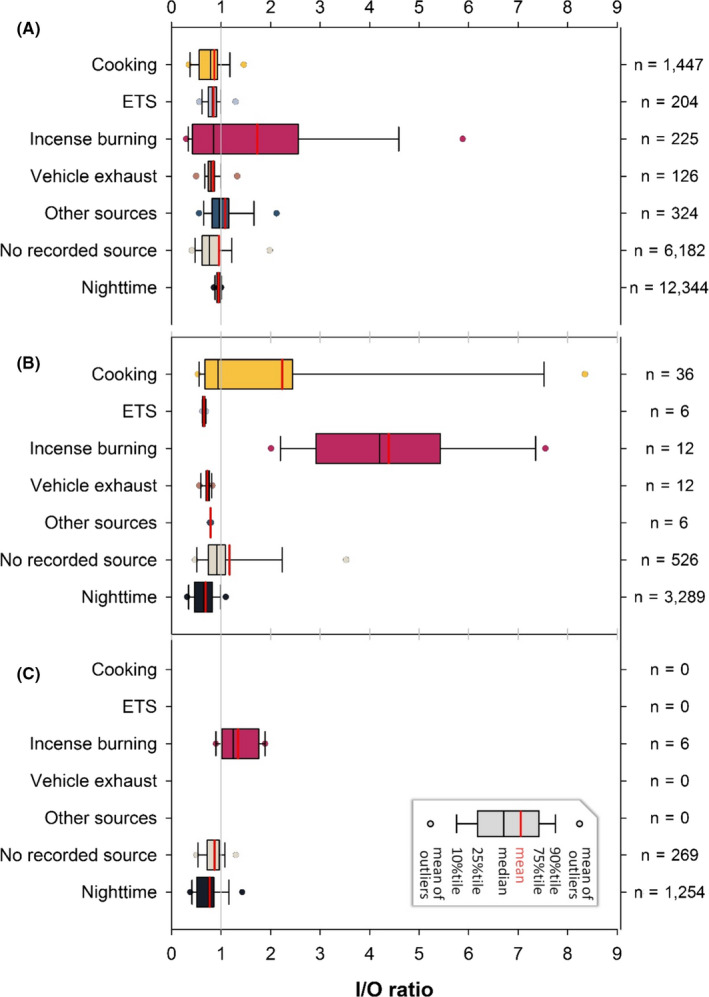
PM_2.5 I/O ratios (5 min) during at‐home periods with different exposure sources under (A) window‐open, (B) window‐closed, and (C) AC‐on; data were from the daytime except for the last category (nighttime)

The source with the highest percentage of PM_2.5 I/O ratios above 1 was incense burning with the highest 75 percentiles, with 2.1, 5.2, and 1.6 for window‐open, window‐closed, and AC‐on, respectively. Under window‐closed and AC‐on conditions, the I/O ratios of incense burning were significantly higher than those of all other sources (p < .05). Another source with high I/O ratios was cooking, with the highest I/O ratio of 11.7 (data not shown) with window‐closed. In contrast, under window‐open condition, the I/O ratios of cooking were significantly lower than those of all other sources (p < .05), presumably due to the combination of window‐open and the use of an exhaust hood (typical practice in Taiwan). These results indicated that ventilation affects I/O ratios differently for different sources.

Under exposure to incense burning or cooking, the window‐closed I/O ratios were significantly higher than those with window‐open (p < .001 for both). Fortunately, most subjects cooked or burned incense with window‐open. On the contrary, most vehicle emission and ETS exposure indoors occurred with window‐open with I/O ratios significantly higher than those with window‐closed (p < .05). This suggests that vehicle exhaust and ETS from outdoors seeped in through the open windows or that the subjects opened windows to vent the ETS in the home. In summary, with observations and TAD records in high temporal resolution, the impacts of sources and ventilation on IAQ have been assessed in great detail, which has been a great challenge.

3.3. PM_2.5 exposure source evaluation

Exposure source contributions were evaluated focusing on PM_2.5 through case evaluations on high‐exposure events and unusual sources, and through statistical analysis of on‐average contributions of frequently occurring sources. Figure 3A‐D shows cases of personal, indoor, and outdoor PM_2.5 with indications of specific exposure sources encountered. The source evaluations are detailed in the following.

FIGURE 3.

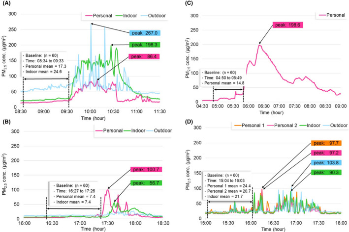
Time series of PM_2.5 exposures (µg/m³, 1‐min resolution) due to different sources: (A) incense burning at home, (B) cooking at home, (C) cooking at bakery, and (D) exposure at a duck‐roasting shop. The baseline concentration (one‐hour mean PM_2.5 concentrations before these events) and the peak levels (the maximum 1‐min observation) during these events are shown. Concurrent indoor and outdoor PM_2.5 levels (µg/m³, 1‐min resolution) are shown whenever available

Figure 3A shows one incense burning event lasting for an hour, with a peak personal PM_2.5 of 86.4 µg/m³. The subject was exposed to incense burning with window‐open starting from 9:34 am and walked outside around 10:32 am After subtracting the corresponding baseline, the maximum PM_2.5 increments due to incense burning were 69.1 µg/m³. Indoor PM_2.5 levels, with a peak of 198.3 µg/m³, were higher than personal PM_2.5 exposures, possibly because the AS‐LUNG‐I set was located closer to the burning spots than the subject. Outdoor PM_2.5 levels were higher than the indoor and personal levels, even before incense burning began, indicating the presence of other sources outdoors. PM_2.5 exposure summation due to worshipping practices was 61.8 (9:34 am‐10:33 am) µg/m³‐h, accounting for 14.5% of PM_2.5 exposures of the subject on that day (event contribution).

Figure 3B‐C shows one event of home cooking for 60 minutes (5:27 pm‐6:26 pm) and another one with exposure to cooking fumes for roughly 145 minutes (5:50 am‐8:14 am) while working in a bakery (without indoor and outdoor monitoring), respectively. Both events occurred under window‐open conditions. The maximum PM_2.5 increments were 93.3 and 183.8 µg/m³ for the home cooking and the bakery events, respectively. PM_2.5 exposure summations due to these cooking events were 26.5 and 260.3 µg/m³‐hr, accounting for 14.0% and 39.6% of PM_2.5 exposures of the subjects on that day, respectively. These two cases showed that high PM_2.5 exposures occurred during cooking practices in modern kitchens without solid fuels. Even though the bakery event occurred in a workplace rather than home, the potential influences of baking practices on PM_2.5 exposures are demonstrated.

Figure 3D shows one event occurring in a duck‐roasting takeaway shop, which has extra indoor and outdoor monitoring since it was the first floor of the household, with the living room on the second floor (Figure 3D). The couple who owned the shop was two of our subjects. There were two very similar personal PM_2.5 exposure levels, close to indoor PM_2.5 levels. The use of wood and charcoal for duck roasting with the addition of their secret spice mixtures without an exhaust hood generated high PM_2.5 indoors, even with window‐open. The maximum PM_2.5 increment was 73.3 µg/m³ and 76.5 µg/m³ for these two subjects. PM_2.5 exposure summations were not calculated since the exposure duration was difficult to determine. Figure 3A‐D shows how AS‐LUNG‐P, AS‐LUNG‐I, and AS‐LUNG‐O can simultaneously assess exposure sources and quantify their incremental contributions to PM_2.5 levels and exposure summations.

Besides a case evaluation, three models were established to quantify the contributions of important factors during at‐home periods, with stepwise regressions. Model 1 shows that indoor and outdoor PM_2.5 levels can explain 74.4% of the variability of personal PM_2.5 exposures in at‐home periods (Table 4A). Outdoor levels, exposure sources, and ventilation statuses without indoor levels can only explain 15.9% of the exposure variability (Model 2). Indoor PM_2.5 alone, affected by those sources shown in Model 3, could explain 74.0% of PM_2.5 exposure variability (partial R ² of indoor PM_2.5 in Model 1). Outdoor PM_2.5 would infiltrate indoors, thus accounting for the highest partial R ² for indoor PM_2.5 (Table 4B). Increments of indoor PM_2.5 levels due to cooking, ETS, incense burning, window‐closed, and AC‐on were 1.34, 2.66, 15.0, −1.56, and −0.947 µg/m³, respectively. Their partial R ² values were not high since these activities occurred only occasionally. Burning incense sticks had the highest incremental contribution and the highest partial R ² (0.022) among them.

TABLE 4.

For at‐home periods, contributions (A) of indoor and outdoor levels to personal PM_2.5 exposures (Model 1), of outdoor levels with indoor sources and ventilation terms to personal PM_2.5 exposures (Model 2), and (B) of outdoor levels with indoor sources and ventilation terms to indoor PM_2.5 (Model 3); PM_2.5 are all at a 5‐min resolution (μg/m³, n = 26 321)

(A)	Model 1 (R 2 = 0.744) (adjusted R 2 = 0.744) a		Model 2 (R 2 = 0.159) (adjusted R 2 = 0.159)
	Dependent variable (personal PM2.5)		Dependent variable (personal PM2.5)
Variables	Coefficient 95% confidence interval	Partial R 2	Coefficient 95% confidence interval	Partial R 2
Intercept	0.855 (0.725, 0.985)*	–	5.34 (5.11, 5.58)*	–
Indoor PM2.5	0.617 (0.612, 0.621)*	0.74	–	–
Outdoor PM2.5	0.0649 (0.0587, 0.0712)*	0.004	0.310 (0.299, 0.321)*	0.116
Cooking	–	–	3.14 (2.67, 3.61)*	0.006
ETS	–	–	3.48 (2.46, 4.50)*	0.002
Incense burning	–	–	10.5 (9.71, 11.4)*	0.021
Window‐closed b	–	–	‐0.987 (−1.32, −0.657)*	0.001
AC‐on b	–	–	‐5.15 (−5.66, −4.65)*	0.014

(B)	Model 3 (R 2 = 0.132) (adjusted R 2 = 0.132)
	Dependent variable (indoor PM2.5)
Variables	Coefficient 95% confidence interval	Partial R 2
Intercept	7.02 (6.70, 7.35)*	–
Outdoor PM2.5	0.406 (0.391, 0.421)*	0.106
Cooking	1.34 (0.689, 1.99)*	0.001
ETS	2.66 (1.26, 4.06)*	<0.001
Incense burning	15.0 (13.8, 16.1)*	0.022
Window‐closed b	‐1.56 (−2.02, −1.11)*	0.002
AC‐on b	‐0.947 (−1.64, −0.253)*	<0.001

^aThe adjusted R ² is equal to R ² in the three models since the sample size was large and the number of independent variables was small.

^bThe reference group of the ventilation type was “window‐open.”

^* p‐value < .001.

4. DISCUSSION

4.1. Applicability of LCS devices

Personal PM_2.5 and PM₁ exposures at 15‐sec resolution were successfully assessed using AS‐LUNG‐P for 26 non‐smoking healthy adults in Taiwan. Being small, lightweight, free of noise and vibration, easy to use, and inconspicuous, AS‐LUNG‐P facilitated subject recruitment, allowed subjects to perform their daily routine as usual, and enabled repeated measurements of 7‐day close‐to‐reality PM_2.5 exposures for each subject. Hence, higher statistical powers with more observations for source evaluation were obtained compared with integrated filter samples or expensive monitors. ⁸ In addition, the high R ² of correction equations, high data collection rates, and the lack of ghost peaks or negative signals in the field campaigns eased the concern of data quality for AS‐LUNG‐P, AS‐LUNG‐I, and AS‐LUNG‐O. The latter two small devices (without noise, vibration, and a conspicuous appearance) did not arouse any complaints from the households and successfully monitored concurrent indoor and outdoor PM_2.5 and PM₁ levels, respectively. These performances demonstrated the applicability of these LCS devices in exposure and IAQ studies.

In the United States and Europe, large‐scale personal PM_2.5 exposure campaigns have been carried out, such as Air Pollution Exposure Distributions within Adult Urban Populations in Europe (EXPOLIS) and the Relationships of Indoor, Outdoor and Personal Air (RIOPA) starting in the late 1990s, ²⁹ , ³⁰ to determine exposure levels in different indoor and outdoor microenvironments. For Asian countries with high ambient PM_2.5 levels for the past 20 years, the lack of such PM_2.5 exposure campaigns was presumably due to the required expensive instruments and resources. The availability of these newly developed LCS devices for PM_2.5 would facilitate the implementation of PM_2.5 exposure campaigns in Asia with much lower costs and evaluate more Asia‐specific exposure sources in indoor and outdoor microenvironments.

Potential applications of LCS devices in IAQ research have been elaborated for unattended large‐scale monitoring and for immediate warning for high pollutant levels. ¹⁹ Some researchers have used LCS devices to assess IAQ, such as Dylos, iKair, and Yun PM sensors used in the United States and China. ³¹ , ³² , ³³ On the other hand, LCS devices were used for PM exposure assessment. For example, Alphasense OPC‐N2 sensors were used in Hong Kong for 73 subjects, ³⁴ another portable aerosol nephelometer in Beijing for 31 subjects, ³⁵ and AS‐LUNG‐P sets in Bandung, Indonesia, for 32 subjects. ³⁶ Those studies also compared sensors against research‐grade instruments such as ours. However, no concurrent home indoor and outdoor monitoring accompanied exposure assessment. To our knowledge, this work is the first one presenting concurrent personal, indoor, and outdoor PM levels with LCS devices. With these concurrent observations and TAD records for multiple subjects and days, important or unusual sources have been identified and evaluated in detail at a relatively low cost.

4.2. PM_2.5 and PM₁ exposure, indoor, and outdoor levels

Previous exposure or IAQ studies sometimes assessed subjects or households on a single day. Whether the particular day represents subjects’ daily routines has been questioned. This work with PM_2.5 and PM₁ personal, indoor, and outdoor levels assessed at multiple days should be free of this concern. Personal, indoor, and outdoor PM_2.5 levels of 26 subjects were in the range of less than 10 µg/m³ to over 200 µg/m³ at a 5‐minutes resolution, similar to the findings of our previous works in Taiwan. ¹³ , ²⁷ Home outdoor PM_2.5 and PM₁ levels were significantly higher than the corresponding home indoor and personal levels, with median I/O and P/O ratios of 0.75 and 0.57 for PM_2.5 at home, respectively, contrary to most of the reported findings (eg, 7, 37). As reviewed by Mohammed et al, ⁷ due to the impacts of indoor sources, most previous studies found I/O ratios higher than 1. Only a few studies showed I/O ratios < 1, ³³ , ³⁸ , ³⁹ with two showing median PM_2.5 I/O ratios similar to ours. One was in China in 2017, with a median I/O ratio of 0.6‐0.75 in 46 naturally ventilated homes when outdoor PM_2.5 is higher than 150 µg/m³. ³³ Another one was in Germany in 2016‐2019, with a median I/O ratio of 0.69 and a mean outdoor PM_2.5 of 13.4‐18.0 µg/m³ for 40 non‐smoking homes. ³⁹ As for P/O ratios, there were few reported in the literature in the past 10 years.

Even with generally higher outdoor levels, personal exposures were significantly affected by indoor sources and ventilation statuses, as in most previous studies. Among those home indoor sources, the sources with the highest PM_2.5 P/I ratios were ETS (0.94 ± 0.54) and cooking (0.91 ± 0.33), demonstrating that these two were the closest exposure sources to the subjects. The median (5‐minutes) PM_2.5 P/I ratio of 0.76 for at‐home periods indicated that the subjects were fortunately not too close to any sources at home most of the time. Even lower P/I ratios during sleep with or without AC‐on further demonstrated PM variations in different rooms (with different sources) of the same households. These results emphasize that personal exposure assessment cannot be substituted by home indoor monitoring. Even with high correlations, indoor PM levels were overestimates of personal PM exposures, since people may avoid the known sources with high awareness or stay in rooms with fewer sources than the living rooms. On the other hand, AS‐LUNG‐I sets could be placed at different rooms in the future to further evaluate variations among different microenvironments within households.

4.3. Evaluation on sources and ventilation statuses

With AS‐LUNG providing a high resolution of PM_2.5 and PM₁ data, plus TAD records, the intensity, frequency, durations, and increments of sources could be assessed in more detail, compared with 24‐hour integrated filter samples. ⁸ The top three frequently occurring household sources of PM_2.5 and PM₁ identified were cooking, ETS, and incense burning. High‐exposure events and special sources were evaluated by quantifying their maximum PM_2.5 exposure increments, PM_2.5 exposure summation, and event contributions via assessing temporal changes in PM_2.5 exposure. Significant contributions of single events to the daily PM_2.5 exposure summation (14.0%‐39.6%) were demonstrated. For frequently occurring sources, the on‐average PM_2.5 contributions were quantified for the entire panel during at‐home periods.

The household source with the highest PM_2.5 I/O (1.44 ± 1.44) and P/O (1.08 ± 1.12) ratios among all single sources and the highest PM_2.5 increments to indoor levels in regression (15.0 µg/m³) was incense burning, consistent with the previous findings that incense burning generated high PM_2.5 levels. ¹¹ , ⁴⁰ We found that one incense stick generated 32.6‐52.7 mg of PM_2.5, higher than one cigarette (14 ± 4 mg) ⁴¹ . Elevated PM_2.5 was found during indoor worshipping practices, especially with window‐closed. ⁴⁰ Burning incense is a ceremonial practice for deity worshipping in Buddhism and Taoism (the two most popular folk religions in Taiwan) and paying respect to ancestors, a time‐honored Chinese tradition. Most senior Taiwanese observe this ritual at home twice a month, while some people even worship twice a day and sometimes accompanying with joss paper burning, resulting in extra PM emissions. ⁴² High frequency and high exposures of this traditional practice may be harmful to their health.

Cooking is the most frequently occurring indoor source in this panel study. Duck roasting with wood and charcoal at one household resulted in a maximum PM_2.5 increment of 76.5 µg/m³, consistent with studies on solid fuels for cooking. ¹⁰ Solid fuels were used by more than 60% of households in Africa and South‐East Asia, 46% in the Western Pacific, 35% in the Eastern Mediterranean, and less than 20% in the Americas and Europe. ¹⁰ The PM exposure contributions from those traditional cooking practices can be assessed by the novel LCS devices. The concern of cooking grease damaging mirrors inside the expensive light‐scattering instruments could be eased due to the cheaper replacement costs of these sensors.

Nevertheless, most Taiwanese households use gas stoves or electrical appliances with kitchen exhaust hoods turned on. High‐exposure cooking events without solid fuels were identified with the maximum PM_2.5 increment of 93.3 µg/m³ and 183.8 µg/m³, even with window‐open. Cuisine practices of stir‐fry, deep‐fry, and baking may be responsible for the high PM emissions. Cooking peaks in modern kitchens have been found to be 1.6‐ to 1.7‐fold above mean PM_2.5 levels in Canada, ³⁸ while the peaks in our results were one order of magnitude higher in personal and indoor PM_2.5 above the background. More effective kitchen exhaust hoods may be needed to further reduce PM levels. Attention in the study of cooking has been paid to solid fuels; our results showed that typical modern cuisine practices with gas stoves or electrical appliances may also generate high PM exposures if not well‐ventilated.

Furthermore, the infiltration of vehicle exhaust into indoor environments was demonstrated by other researchers with traffic‐related elements found indoors. ⁷ Asian cities usually have high population densities, and residences are packed along the busy streets. 12.3% of residents in metropolitan Taipei actually live on the first or second floor, within 5 m from municipal roads. ⁴³ Thus, it is no surprise that our subjects recorded exposure to vehicle emissions at home with low I/O ratios in Figure 2.

Ventilation affecting personal exposure and IAQ at home was demonstrated with indoor sources and building protection as two push‐and‐pull factors, as discussed by others. ⁷ , ³³ , ³⁷ , ³⁸ In this work, I/O ratios above 1 with window‐closed indicated high impacts of indoor sources (Figure 2), while window‐closed conditions typically reduced at‐home exposures and indoor levels (Table 4), indicating buildings’ shielding effects. These studied households all had natural ventilation (windows and doors); for other households with mechanical ventilation systems, the efficiency of the ventilation is another important factor to consider. In addition, outdoor PM levels higher than the concurrent indoor levels indicated that the outdoor ambient air in Taiwan is generally more polluted than the air indoors. Behavior change recommendations can be formulated on the basis of these scientific findings and actions can be triggered with the assistance of LCS devices. IAQ experts all know that closing windows prevents outdoor PM_2.5 from entering a building, and opening windows vents PM_2.5 generated indoors. However, ordinary citizens do not always know when to take action. With concurrent real‐time monitoring of indoor and outdoor PM_2.5, wireless transmission, and a screen display, people can open (or close) windows when indoor levels are higher (or lower) than those outdoors to reduce exposure and the associated health risks. Our work demonstrates the feasibility of applying these LCS devices in citizen science for the protection of public health.

4.4. Limitations

Two issues are associated with the application of AS‐LUNG sets. First, the collocated comparison with GRIMM was conducted for each set to ensure data quality, requiring substantial manpower and expenses. Although these devices were of low cost, the required expenses for their application to research were by no means trivial. In addition, AS‐LUNG‐P and AS‐LUNG‐I are not entirely enclosed. Thus, they were not waterproof and should be protected against water.

There are other limitations in this work. Firstly, larger errors were encountered for observations >150 µg/m³. However, the percentages of these high values were small; thus, the effect of correction errors on the statistical estimates is insignificant. Secondly, certain battery compatibility issues caused roughly a 4%‐5% data loss for the three versions of AS‐LUNG. This should not affect our findings since data loss was random. Thirdly, I/O ratios were above 1 for some observations without sources recorded in TADs, indicating the possibility that subjects forgot about, ignored, or did not know about certain sources. Thus, certain exposure events might be neglected in current analysis. Finally, we did not have detailed information on the usage of air cleaners to assess the influence of air cleaning. This could be improved by adding “air cleaning usage” in TADs.

5. CONCLUSIONS

This work is the first to present concurrent personal, indoor, and outdoor PM_2.5 and PM₁ measurements with LCS devices. It demonstrated the successful application of three versions of LCS devices to assess source contributions in exposure and IAQ studies, that is, AS‐LUNG‐P, AS‐LUNG‐I, and AS‐LUNG‐O for personal exposure, indoor, and outdoor monitoring, respectively. To ensure data quality, correction equations for converting their readings into GRIMM‐comparable observations were established with a high R ² up to 0.998 using collocated comparisons. In field campaigns, high time resolution of close‐to‐reality PM_2.5 and PM₁ exposures of subjects on multiple days was assessed using AS‐LUNG‐P, which is small, lightweight, free of noise and vibration, easy to use, and inconspicuous. With concurrent indoor and outdoor monitoring at households and TAD records of 26 healthy adults, evaluation was carried out on the intensity, frequency, duration, and contribution of important indoor sources, especially in Asian households. Traditional worshipping practices, cooking with solid fuels, and cooking in modern kitchens (gas stoves and electrical appliances) may result in high PM_2.5 increments of 69.1‐183.8 µg/m³ with event contributions of 14.0%‐39.6% of daily PM_2.5 exposures. Behavior change recommendations could be formulated according to these findings; actions, such as when to open/close windows, could be triggered with the assistance of LCS devices, demonstrating their application potential in citizen science. The methodology used can be applied to assessing incremental contribution of other sources to PM_2.5 and PM₁ exposures in other countries. In particular, for high PM Asian countries with exposure sources distinct from those in Western countries, LCS devices can be employed to identify important unknown exposure sources and quantify their incremental contributions.

CONFLICT OF INTEREST

The authors declare that they have no actual or potential competing financial interests.

AUTHOR CONTRIBUTION

Shih‐Chun Candice Lung: Conceptualization (lead); Funding acquisition (lead); Methodology (lead); Project administration (lead); Supervision (lead); Writing‐original draft (lead); Writing‐review & editing (lead). Ming‐Chien Mark Tsou: Formal analysis (lead); Software (lead); Validation (lead); Writing‐original draft (supporting); Writing‐review & editing (equal). Shu‐Chuan HU: Conceptualization (supporting); Investigation (equal); Project administration (lead); Visualization (equal); Writing‐review & editing (equal). Yu‐Hui Hsieh: Data curation (lead); Investigation (lead); Writing‐review & editing (supporting). Wen‐Cheng Vincent Wang: Conceptualization (supporting); Data curation (equal); Project administration (supporting); Writing‐review & editing (supporting). Chen‐Kai Shui: Data curation (supporting); Investigation (equal); Visualization (supporting). Chee‐Hong Tan: Investigation (equal); Visualization (supporting).

Peer Review

The peer review history for this article is available at https://publons.com/publon/10.1111/ina.12763.

Supporting information

Appendix S1

DATA AVAILABILITY STATEMENT

The data that support the findings of this study are available on request from the corresponding author. The data are not publicly available due to privacy or ethical restrictions.

REFERENCES

- 1. IARC . IARC Scientific Publication no. 161: Air Pollution and Cancer. International Agency for Research on Cancer (IARC); 2013. http://publications.iarc.fr/Book‐And‐Report‐Series/Iarc‐Scientific‐Publications/Air‐Pollution‐And‐Cancer‐2013 [Google Scholar]
- 2. Forouzanfar MH, Afshin A, Alexander LT, et al. Global, regional, and national comparative risk assessment of 79 behavioural, environmental and occupational, and metabolic risks or clusters of risks, 1990–2015: a systematic analysis for the global burden of disease study 2015. Lancet. 2016;388(10053):1659‐1724. [DOI] [PMC free article] [PubMed] [Google Scholar]
- 3. Institute for Health Metrics and Evaluation, Global Burden of Disease (GBDx Results Tool). 2020, http://ghdx.healthdata.org/gbd‐results‐tool Accessed March 7, 2020.
- 4. Roser M, Ritchie H. Indoor Air Pollution; 2014. https://ourworldindata.org/indoor‐air‐pollution. Accessed March 7, 2020. [Google Scholar]
- 5. van Donkelaar A, Martin RV, Brauer M, Boys BL. Use of satellite observations for long‐term exposure assessment of global concentrations of fine particulate matter. Environ Health Perspect. 2015;123(2):135‐143. [DOI] [PMC free article] [PubMed] [Google Scholar]
- 6. Morawska L, Afshari A, Bae GN, et al. Indoor aerosols: from personal exposure to risk assessment. Indoor Air. 2013;23(6):462‐487. [DOI] [PubMed] [Google Scholar]
- 7. Mohammed MOA, Song WW, Ma WL, et al. Trends in indoor‐outdoor PM2.5 research: A systematic review of studies conducted during the last decade (2003–2013). Atmos Pollut Res. 2015;6(5):893‐903. [Google Scholar]
- 8. Lung SCC, Mao IF, Liu LJS. Residents' particle exposures in six different communities in Taiwan. Sci Total Environ. 2007;377(1):81‐92. [DOI] [PubMed] [Google Scholar]
- 9. Lung SCC, Hsiao PK, Wen TY, Liu CH, Fu CB, Cheng YT. Variability of intra‐urban exposure to particulate matter and CO from Asian‐type community pollution sources. Atmos Environ. 2014;83:6‐13. [Google Scholar]
- 10. Bonjour S, Adair‐Rohani H, Wolf J, et al. Solid fuel use for household cooking: country and regional estimates for 1980–2010. Environ Health Perspect. 2013;121(7):784‐790. [DOI] [PMC free article] [PubMed] [Google Scholar]
- 11. Lung SCC, Hu SC. Generation rates and emission factors of particulate matter and particle‐bound polycyclic aromatic hydrocarbons of incense sticks. Chemosphere. 2003;50(5):673‐679. [DOI] [PubMed] [Google Scholar]
- 12. Jerrett M, Burnet RT, Ma R, et al. Spatial analysis of air pollution and mortality in Los Angeles. Epidemiology. 2006;17(6):S69. [DOI] [PubMed] [Google Scholar]
- 13. Lung SCC, Chen N, Hwang JS, et al. Panel study using novel sensing devices to assess associations of PM2.5 with heart rate variability and exposure sources. J Expo Sci Environ Epidemiol. 2020;30:937–948. 10.1038/s41370-020-0254-y [DOI] [PubMed] [Google Scholar]
- 14. Klepeis NE, Nelson WC, Ott WR, et al. The National Human Activity Pattern Survey (NHAPS): a resource for assessing exposure to environmental pollutants. J Expo Anal Environ Epidemiol. 2001;11(3):231‐252. [DOI] [PubMed] [Google Scholar]
- 15. Tang CS, Wu TY, Chuang KJ, et al. Impacts of in‐cabin exposure to size‐fractionated particulate matters and carbon monoxide on changes in heart rate variability for healthy public transit commuters. Atmosphere. 2019;10(7):17. [Google Scholar]
- 16. Lung SCC, Kao MC. Worshippers' exposure to particulate matter in two temples in Taiwan. J Air Waste Manage Assoc. 2003;53(2):130‐135. [DOI] [PubMed] [Google Scholar]
- 17. Chen LJ, Ho YH, Lee HC, et al. An open framework for participatory PM2.5 monitoring in smart cities. IEEE Access. 2017;5:14441‐14454. [Google Scholar]
- 18. Snyder EG, Watkins TH, Solomon PA, et al. The changing paradigm of air pollution monitoring. Environ Sci Technol. 2013;47(20):11369‐11377. [DOI] [PubMed] [Google Scholar]
- 19. Lowther SD, Jones KC, Wang XM, Whyatt JD, Wild O, Booker D. Particulate matter measurement indoors: a review of metrics, sensors, needs, and applications. Environ Sci Technol. 2019;53(20):11644‐11656. [DOI] [PubMed] [Google Scholar]
- 20. Clements AL, Griswold WG, Abhijit RS, et al. Low‐Cost air quality monitoring tools: from research to practice (a workshop summary). Sensors. 2017;17(11):20. [DOI] [PMC free article] [PubMed] [Google Scholar]
- 21. Badura M, Batog P, Drzeniecka‐Osiadacz A, Modzel P. Evaluation of Low‐Cost sensors for ambient PM2.5 monitoring. J Sens. 2018;2018:1–16. [Google Scholar]
- 22. Wang Y, Li JY, Jing H, Zhang Q, Jiang JK, Biswas P. Laboratory evaluation and calibration of three Low‐Cost particle sensors for particulate matter measurement. Aerosol Sci Technol. 2015;49(11):1063‐1077. [Google Scholar]
- 23. Kelly KE, Whitaker J, Petty A, et al. Ambient and laboratory evaluation of a low‐cost particulate matter sensor. Environ Pollut. 2017;221:491‐500. [DOI] [PMC free article] [PubMed] [Google Scholar]
- 24. Sayahi T, Butterfield A, Kelly KE. Long‐term field evaluation of the Plantower PMS low‐cost particulate matter sensors. Environ Pollut. 2019;245:932‐940. [DOI] [PubMed] [Google Scholar]
- 25. Zheng TS, Bergin MH, Johnson KK, et al. Field evaluation of low‐cost particulate matter sensors in high‐and low‐concentration environments. Atmos Meas Tech. 2018;11(8):4823‐4846. [Google Scholar]
- 26. Sayahi T, Kaufman D, Becnel T, et al. Development of a calibration chamber to evaluate the performance of low‐cost particulate matter sensors. Environ Pollut. 2019;255:9. [DOI] [PMC free article] [PubMed] [Google Scholar]
- 27. Lung SCC, Wang WCV, Wen TYJ, Liu CH, Hu SC. A versatile low‐cost sensing device for assessing PM2.5 spatiotemporal variation and quantifying source contribution. Sci Total Environ. 2020;716:137145. [DOI] [PubMed] [Google Scholar]
- 28. Wang WCV, Lung SCC, Liu CH, Shui CK. Laboratory evaluating of correction equations with multiple choices for seed low‐cost particle sensing devices in sensor networks. Sensors. 2020;20(13):3661. [DOI] [PMC free article] [PubMed] [Google Scholar]
- 29. Koistinen KJ, Kousa A, Tenhola V, et al. Fine particle (PM2.5) measurement methodology, quality assurance procedures, and pilot results of the EXPOLIS study. J Air Waste Manage Assoc. 1999;49(10):1212‐1220. [DOI] [PubMed] [Google Scholar]
- 30. Meng QY, Spector D, Colome S, Turpin B. Determinants of indoor and personal exposure to PM2.5 of indoor and outdoor origin during the RIOPA study. Atmos Environ. 2009;43(36):5750‐5758. [DOI] [PMC free article] [PubMed] [Google Scholar]
- 31. Han I, Symanski E, Stock TH. Feasibility of using low‐cost portable particle monitors for measurement of fine and coarse particulate matter in urban ambient air. J Air Waste Manage Assoc. 2017;67:330‐340. [DOI] [PMC free article] [PubMed] [Google Scholar]
- 32. Hegde S, Min KT, Moore J, et al. Indoor household particulate matter measurements using a network of low‐cost sensors. Aerosol Air Qual Res. 2020;20:381‐394. [Google Scholar]
- 33. Dai X, Liu J, Li X, Zhao L. Long‐term monitoring of indoor CO2 and PM2.5 in Chinese homes: Concentrations and their relationships with outdoor environments. Building and Environ. 2018;144:238‐247. [Google Scholar]
- 34. Yang FH, Lau CF, Tong VWT, et al. Assessment of personal integrated exposure to fine particulate matter of urban residents in Hong Kong. J Air Waste Manage Assoc. 2019;69:47‐57. [DOI] [PubMed] [Google Scholar]
- 35. Liang L, Gong P, Cong N, Li ZC, Zhao Y, Chen Y. Assessment of personal exposure to particulate air pollution: the first result of City Health Outlook (CHO) project. BMC Public Health. 2019;19:12. [DOI] [PMC free article] [PubMed] [Google Scholar]
- 36. Sinaga D, Setyawati W, Cheng FY, Lung SCC. Investigation on daily exposure to PM2.5 in Bandung City, Indonesia using low‐cost sensor. J Expo Sci Environ Epidemiol. 2020;30:1001–1012. 10.1038/s41370-020-0256-9 [DOI] [PubMed] [Google Scholar]
- 37. Clements N, Keady P, Emerson JB, Fierer N, Miller SL. Seasonal variability of airborne particulate matter and bacterial concentrations in Colorado homes. Atmosphere. 2018;9:18. [Google Scholar]
- 38. Wheeler AJ, Wallace LA, Kearney J, et al. Personal, indoor, and outdoor concentrations of fine and ultrafine particles using continuous monitors in multiple residences. Aerosol Sci Technol. 2011;45:1078‐1089. [Google Scholar]
- 39. Zhao J, Birmili W, Wehner B, et al. Particle mass concentrations and number size distributions in 40 homes in Germany: indoor‐to‐outdoor relationships, diurnal and seasonal variation. Aerosol Air Qual Res. 2020;20:576‐589. [Google Scholar]
- 40. Lung SCC, Kao MC, Hu SC. Contribution of incense burning to indoor PM10 and particle‐bound polycyclic aromatic hydrocarbons under two ventilation conditions. Indoor Air. 2003;13(2):194‐199. [DOI] [PubMed] [Google Scholar]
- 41. Ozkaynak H, Xue J, Spengler J, Wallace L, Pellizzari E, Jenkins P. Personal exposure to airborne particles and metals: results from the particle TEAM study in Riverside, California. J Exposure Anal Environ Epidemiol. 1996;6(1):57‐78. [PubMed] [Google Scholar]
- 42. Yang HH, Jung RC, Wang YF, Hsieh LT. Polycyclic aromatic hydrocarbon emissions from joss paper furnaces. Atmos Environ. 2005;39(18):3305‐3312. [Google Scholar]
- 43. Wu CD, Lung SCC. Applying GIS and fine‐resolution digital terrain models to assess three‐dimensional population distribution under traffic impacts. J Expo Sci Environ Epidemiol. 2012;22(2):126‐134. [DOI] [PubMed] [Google Scholar]
Associated Data
This section collects any data citations, data availability statements, or supplementary materials included in this article.
Supplementary Materials