Multiobjective Optimization of Mixed-Integer Linear Programming Problems: A Multiparametric Optimization Approach

Abstract

Industrial process systems need to be optimized, simultaneously satisfying financial, quality and safety criteria. To meet all those potentially conflicting optimization objectives, multiobjective optimization formulations can be used to derive optimal trade-off solutions. In this work, we present a framework that provides the exact Pareto front of multiobjective mixed-integer linear optimization problems through multiparametric programming. The original multiobjective optimization program is reformulated through the well-established ϵ-constraint scalarization method, in which the vector of scalarization parameters is treated as a right-hand side uncertainty for the multiparametric program. The algorithmic procedure then derives the optimal solution of the resulting multiparametric mixed-integer linear programming problem as an affine function of the ϵ parameters, which explicitly generates the Pareto front of the multiobjective problem. The solution of a numerical example is analytically presented to exhibit the steps of the approach, while its practicality is shown through a simultaneous process and product design problem case study. Finally, the computational performance is benchmarked with case studies of varying dimensionality with respect to the number of objective functions and decision variables.

Graphical Abstract

1. Introduction

Multiobjective optimization problems are inherent in many fields, including engineering,^1–8 supply chain management,^9–11 and economics^12,13 where the decision maker is interested in minimizing several cost criteria that directly compete with each other. Examples of these competing objectives include maximizing profits, maximizing safety, and minimizing environmental impacts. The challenge associated with multiobjective optimization programs lies in handling these competing cost criteria simultaneously. Unlike optimization formulations with a single objective function, in multiobjective optimization the decision maker will choose a solution among many equally optimal solutions that will satisfy their priorities concerning the competing objectives. In this latter case, an optimal solution occurs at any feasible point in which all objectives are minimized such that no other feasible solution exists that could further improve an objective function without worsening another objective function. These optimal decision variables are termed Pareto points and the union of the corresponding objective function values that creates the full representation of the trade-off analysis between the competing cost criteria forms the Pareto front.

The benefit of having the full Pareto front of a multiobjective optimization problem is substantial since it allows the decision maker to select its preferred conflicting optimal solution. However, typically multiobjective problems have infinitely many optimal solutions and hence require substantial computational effort to be solved.¹⁴ Therefore, the derivation of the exact structure of the Pareto front has frequently been based on approximation techniques.^15,16 The computational challenges of solving multiobjective optimization problems are amplified when more than two objective functions are considered. This is also one of the reasons why researchers have primarily solved biojective and triobjective optimization problems.^17,18 When integer variables are also considered to be part of the multiobjective optimization formulation, the challenges in deriving the full Pareto front are enhanced due to the discontinuity and nonconvexity of the Pareto front.

Hence, the focus of this contribution is to provide an exact explicit representation of the Pareto front for multiobjective mixed-integer linear programming problems given in the following form:

$$\begin{array}{l}\underset{x,y}{\text{min}}\left[c_{1}x+d_{1}y,c_{2}x+d_{2}y,\dots ,c_{p}x+d_{p}y\right]\\ \begin{array}{ll}\text{s.t.}\hfill & A_{1}x+E_{1}y\le b_1\hfill \\ \hfill & A_{2}x+E_{2}y=b_2\hfill \\ \hfill & x\in X\subseteq {ℝ}^n\hfill \\ \hfill & y\in Y={\left\{0,1\right\}}^m\hfill \end{array}\end{array}$$ (1)

where c₁, c₂,…, c_p are the row vector coefficients of the continuous variables, and d₁, d₂,…, d_p are the row vector coefficients of the binary variables of the p objective functions. The inequality constraints are described by the matrices A₁, E₁ and the vector b₁, the equality constraints by the matrices A₂, E₂ and the vector b₂, while X and Y define the sets of the continuous and binary optimization variables, respectively.

1.1. Solution Strategies

Among many different solution strategies that exist for multibojective mixed-integer linear optimization problems, and multiobjective decision making in general, two of the most widely adopted techniques are the ϵ-constraint method and the weighted-sum method.¹⁴ The ϵ-constraint method reformulates the multiobjective optimization problem to a single objective structure by assigning all but one of the objective functions in the constraint set of the problem. Even though the size of the problem increases, theoretically Pareto fronts of any class of multiobjective problems can be found using this approach.¹⁹ In the weighted-sum method on the other hand, prioritization coefficients are utilized for each objective function, and a single objective optimization problem is solved. The weighted-sum method does not lead to a more complex problem formulation as compared to the ϵ-constraint method because solely the latter introduces additional inequality constraints for the objective functions which are moved to the constraint set. However, the drawback of the weighted-sum method is that it cannot find all Pareto solutions if the problem is nonconvex or discontinuous.¹⁴ Another research challenge associated with the generation of the Pareto front of multiobjective optimization problems is that as the problem size grows, developing the full Pareto front becomes prohibitive. For this reason, solution strategies for omitting certain objective functions to reduce the computational burden have been explored.²⁰

Within the context of this work, we specifically focus on linear multiobjective problems with both continuous and binary decision variables. The need to address the solution of industrially-relevant mulitobjective mixed-integer linear optimizations problems is prevalent particularly for the design and operation problems in chemical and process engineering. Additionally, this class of problems represents a common problem formulation for many other applications, and developing the Pareto front within a suitable time frame is increasingly difficult as the problem size grows. Furthermore, a key challenge associated with these formulations is that they could have disconnected and nonconvex Pareto optimal sets¹⁴ which require suitable algorithms to develop the Pareto front. Several algorithms have been proposed in the open literature for the solution of multiobjective mixed-integer linear programming problems. Initial efforts focused on enumerating schemes,^21,22 whereas more recent efforts focused on branch-and-bound algorithms,^23–25 triangle splitting,²⁶ ϵ-Tabu-constraint algorithm,²⁷ one direction search method,²⁸ slicing with adaptive steps search method,²⁹ grid generation¹⁸ for approximating Pareto points, AUGMECON,^19,30 PolySCIP,³¹ and the GoNDEF algorithms.³² Yet, many of these techniques require to develop effective branching and fathoming strategies,^23–25 rely on a generating grid points and/or solving subproblems to map the Pareto solution,^30,32 and solely be applicable to bi and triobjective cases^23,25–29 which significantly limit their use in higher-dimensional case studies.

1.2. Multiobjective Optimization and Multiparametric Programming

Multiparametric programming has also been employed as a useful tool for the development of the Pareto front of multiobjective optimization problems, through the generation of explicit expressions of the Pareto front as a function of the objectives.³³ Papalexandri and Dimkou³⁴ have proposed one of the first notable contributions to address multiobjective convex mixed-integer nonlinear optimization problems through multiparametric programming. The authors have developed an iterative algorithm to construct an approximate Pareto front for simultaneous process synthesis/planning and product/process design problems under uncertainty. Hugo et al.³⁵ have conceptualized the use of recently emerging exact multiparametric programming algorithms for a systematic evaluation of the economic and environmental impacts of material selection in process design. Dua et al.³⁶ have developed a multiobjective explicit model predictive controller to regulate the insulin injection for people with type 1 diabetes by controlling the blood glucose concentration, while in³⁷ the authors have employed the weighted-sum method to derive the Pareto front of explicit model predictive control problems. Oberdieck and Pistikopoulos³⁸ have proposed an algorithm to develop an approximate and explicit expression for multiobjective optimization problems with quadratic objective functions and linear constraints by reformulating the problem into a multiparametric quadratically constrained quadratic program (mpQCQP). More recently, Charitopoulos and Dua³⁹ have utilized multiparametric linear programming (mpLP) to solve linear multiobjective optimization problems under uncertainty. Both of the latter approaches utilized the ϵ-constraint approach.

1.3. Key Contributions

In this work, multiparametric programming is utilized to explicitly develop the exact Pareto front of multiobjective mixed-integer linear programming problems. The benefits of the proposed approach are the the following:

1. All objective functions are derived as an affine function of the ϵ parameters, significantly reducing the computational cost by avoiding the need to solve repetitive optimization problems for different objective prioritizations.

2. The full Pareto front is exactly derived due to the explicit nature of the solution, even for cases when the Pareto front is discontinuous.

3. A relatively large number of objective functions (> 4) are efficiently handled through multiparametric programming, compared to many other available approaches that are limited to formulations with two or three objective functions.

4. Weakly Pareto solutions are readily identified and can be potentially discarded.

The remainder of the manuscript is organized as follows: Section 2 presents the proposed framework and methodology for developing the Pareto front using multiparametric programming. Aside from a numerical example in Section 3, a case study of a simultaenous process and product design problem is exhibited in Section 4 to showcase the applicability of our multiobjective optimization approach in practical problems. Moreover, an extensive computational study is presented in Section 5 to evaluate the performance of the aforementioned strategy for different problem sizes. Finally, Section 6 concludes this work.

2. Methodology

This work addresses the explicit generation of the Pareto front of the multiobjective mixed-integer linear optimization problem as presented in (1). Assume that the i^th objective function of (1) is defined as f_i = c_ix + d_iy. The exact optimal solution of this problem, in other words, the set of optimal Pareto solutions, is defined by Miettinen¹⁴ as follows:

Pareto Optimality:

A decision vector ${\left[x^{*T},y^{*T}\right]}^T$ is Pareto optimal if there does not exist any other decision vector [x^T , y^T]^T such that f_i(x, y) ≤ f_i(x*, y*) ∀i = 1, …p, and f_j(x, y) < f_j(x*, y*) for at least one index j.

In the case where a change causes an improvement at one objective function, while another objective function is unchanged, is termed a weakly Pareto solution. For the solution of Problem (1), the ϵ-constraint method is utilized. In this solution strategy, a single objective function of arbitrary choice is optimized, by incorporating the other objective functions of the problem as constraints. Note that the proposed strategy provides the exact global solution of Problem (1). If a different set of objective functions is chosen to be part of the constraint set of the problem, the generated Pareto front will be exactly the same, since the problem is solved to global optimality.⁴⁰ Hence, Problem (1) is reformulated with p − 1 additional inequality constraints as shown in Problem (2)

$$\begin{array}{ll}\underset{x,y}{\text{min}}\hfill & c_{1}x+d_{1}y\hfill \\ \hfill \text{s.t.}\hfill & c_{2}x+d_{2}y\le {ϵ}_2\hfill \\ \hfill & c_{3}x+d_{3}y\le {ϵ}_3\hfill \\ \hfill & \dots \hfill \\ \hfill & c_{p}x+d_{p}y\le {ϵ}_p\hfill \\ \hfill & A_{1}x+E_{1}y\le b_1\hfill \\ \hfill & A_{2}x+E_{2}y=b_2\hfill \\ \hfill & {ϵ}^L\le ϵ\le {ϵ}^U\hfill \\ \hfill & x\in X\subseteq {ℝ}^n\hfill \\ \hfill & y\in Y={\left\{0,1\right\}}^m\hfill \end{array}$$ (2)

Here, the vector $ϵ={\left[{ϵ}_2,{ϵ}_3,\dots ,{ϵ}_p\right]}^T\in {ℝ}^{p-1}$ defines the upper bound for each objective function in the constraint set. The value of the vector ϵ vector is allowed to exist between the vector of lower bounds ϵ^L, and the vector of upper bounds ϵ^U. The set of Pareto optimal solutions can be generated through parametric variation of the right-hand side of the ϵ constraints of Problem (2). Specifically, the resulting multiobjective mixed-integer linear program is a multiparametric mixed-integer linear programming (mpMILP) problem of the form

$$\begin{array}{ll}\underset{x,y}{\text{min}}\hfill & cx+dy\hfill \\ \text{s.t.}\hfill & Ax+Ey\le b+F\theta \hfill \\ \hfill & x\in X\subseteq {ℝ}^n\hfill \\ \hfill & y\in Y={\left\{0,1\right\}}^m\hfill \\ \hfill & \theta \in \Theta :=\left\{\theta \in {ℝ}^w\mid P_A\theta \le P_b\right\}\hfill \end{array}$$ (3)

where the row vector weights of the objective function are $c\in {ℝ}^{1\times n}$, $d\in {ℝ}^{1\times m}$, and $A\in {ℝ}^{q\times n}$, $E\in {ℝ}^{q\times m}$, $F\in {ℝ}^{q\times w}$, while $b\in {ℝ}^{q\times 1}$. The set Θ is the feasible set of the uncertain parameters of the problem, defined by the matrices $P_A\in {ℝ}^{r\times w}$ and $P_b\in {ℝ}^{r\times 1}$. In our case, the dimension of the uncertainty vector, w, is equal to p − 1.

The selection of the lower and upper bound of the ϵ-parameters is completed through the payoff table as follows: the lower bound is found by minimizing individually each objective function, while the upper bound is calculated by evaluating the value of the other objective functions for the aforesaid minimizations and selecting their maximum value. By treating the multiobjective optimization problem as a multiparametric programming problem, its solution can be readily obtained by expressing the optimal solution as an explicit function of the uncertain ϵ parameters. As a result, the computational complexity of generating the Pareto front is alleviated, since the optimal solution at any ϵ value can be calculated by a simple function evaluation. This is a major benefit since the computation of the Pareto front is computationally expensive.^14,19 However, for the class of problems that we are concerned in this work, and as it was pointed out in¹⁹ the ϵ-constraint method offers significant advantages compared to the weighted-sum method, such as the avoiding of scaling of the objective functions which can have a strong influence in the obtained results.

The solution of Problem (3) is described by the different active sets for different parameter realizations, resulting in partitions of the parameter space where each of these active sets remains active. These partitions — the critical regions — for our present study are piecewise linear because the objective function does not include any parameters in its representation.⁴⁰ Hence, since the problem is described by linear functions, the optimal solution of the problem is a piecewise affine function in Θ, which leads to a piecewise affine description of the optimal objective function, or the Pareto front.

Multiple algorithmic strategies have been proposed in the literature to solve mpMILPs.^41–48 In this work, the algorithm proposed by Acevedo and Pistikopoulos is utilized.⁴⁰ This is a well-established method that provides the exact global solution of an mpMILP problem, leading to the exact derivation of the Pareto front of Problem (1). The solution approach proposes a multiparametric branch & bound (mpB&B) approach, in a similar spirit with branch & bound for deterministic optimization programs. At each node of the enumeration tree, an mpLP is solved and subsequently improving lower and upper bounds are calculated. At node i of the B&B tree, there is a set of k corresponding critical regions CR_k,i ∈ Θ_i, and hence a comparison procedure is required to determine a single optimal multiparametric solution for each parameter realization. Additionally, node-pruning criteria are employed to partially alleviate the computational complexity of the proposed approach. The solution algorithm of Problem (1) is presented in Figure 1.

Figure 1:

A branch a bound-based algorithm for the solution of Problem (1).

The solution of an mpMILP has the following form, where the overall feasible space Θ is partitioned in K polytopic critical regions

$$\begin{array}{r}\hfill x^{*}=V_k{\theta }^{*}+r_k,\\ \hfill y^{*}=y_k,\end{array}\}{\theta }^{*}\in C{R}^k=C{R}_A^k\theta \le C{R}_b^k\}$$ (4)

where V_k is the matrix multiplying the parameter vector for the k^th region and r_k is a constant. Hence, the optimal solution is obtained as an explicit function of the parameter θ, and as a result, the computational effort to generate the Pareto front is alleviated. The aforementioned algorithmic approach is implemented through the Parametric OPtimization Toolbox,⁴⁹ which is readily available at http://parametric.tamu.edu/POP/. The overall framework for the solution of multiobjective mixed-integer linear optimization problems is summarized in Table 1. Note that any other mpMILP algorithm can be utilized in the proposed framework. Also, approximation techniques exist for the description of multiparametric programming with nonlinear constraints, by reformulating them through a mixed-integer linear formulation.^50,51 Hence, the proposed methodology can be applied even for problems with nonlinear constraints if an approximation step has preceded, but that represents a future study.

Table 1:

Framework for the solution of multiobjective mixed-integer linear optimization problems.

Step 1: Reformulate the general multiobjective mixed-integer linear optimization problem of the form of Problem (1) to the form shown in Problem (2) using the ∊-constraint method.

Step 2: Calculate the lower and upper bounds for the ∊ parameters of the ∊-constraint formulation by minimizing the individual objectives for the lower bounds, and by evaluating the value of the other objectives and selecting the maximum value for the upper bounds.

Step 3: Reformulate Problem (2) to a multiparametric programming problem (3).

Step 4: Solve the resulting multiparametric programming problem using the algorithm proposed by Acevedo and Pistikopoulos.40

Step 5: Identify weakly Pareto solutions and the corresponding critical regions if at least one objective function is not a parametric function of all ∊ parameters.

Step 6: Obtain the Pareto front and the optimal solution as an explicit function of the ∊ parameters.

It is important to note that the ϵ-constraint method guarantees the discovery of weakly optimal solutions, and further guarantees the Pareto optimality if and only if each objective function is equal to the corresponding ϵ parameter. A key benefit of the proposed approach is that it allows for the explicit identification of regions that are formed by weakly Pareto solutions. This is a consequence of the fact that if at least one of the objective functions does not change as a function of ϵ all parameters, it means that one change in one of the objectives will not be reflected in a change in another objective. Hence, it can be concluded that if there is a region with at least one of the objective function being not a parametric function of one ϵ, while there exist other which are, then that region is formed by a weakly Pareto solution, and as a result, it can be either kept or discarded from the Pareto front description.

The developed approach is analytically applied to a numerical example, along with an implementation to a simultaneous process and product design problem, and a computational study, and are presented in the following sections.

3. Numerical Example

Consider the following MIMOO problem:

$$\begin{array}{ll}\underset{x_1,x_2,y_1,y_2}{\text{min}}\hfill & \left[0.20x_1-0.48x_2-55y_1-20.7y_2,11.01x_1+0.49x_2+52.4y_1+24.8y_2\right]\hfill \\ \hfill \text{s.t.}\hfill & 0.07x_1-1x_2\le 1.78\hfill \\ \hfill & -0.87x_1-0.50x_2+0.02y_2\le 0.05\hfill \\ \hfill & y_1+y_2\le 1\hfill \\ \hfill & 0\le x_1\le 100\hfill \\ \hfill & 0\le x_2\le 100\hfill \\ \hfill & y_1,y_2\in {\{0,1\}}^m\hfill \end{array}$$ (5)

Problem (5) is reformulated through the ϵ-constraint method as follows

$$\begin{array}{ll}\underset{x_1,x_2,y_1,y_2}{\text{min}}\hfill & 0.20x_1-0.48x_2-55y_1-20.7y_2\hfill \\ \hfill \text{s.t.}\hfill & 11.01x_1+0.49x_2+52.4y_1+24.8y_2\le ϵ\hfill \\ \hfill & 0.07x_1-1x_2\le 1.78\hfill \\ \hfill & -0.87x_1-0.50x_2+0.02y_2\le 0.05\hfill \\ \hfill & y_1+y_2\le 1\hfill \\ \hfill & {ϵ}^L\le ϵ\le {ϵ}^U\hfill \\ \hfill & 0\le x_1\le 100\hfill \\ \hfill & 0\le x_2\le 100\hfill \\ \hfill & y_1,y_2\in {\{0,1\}}^m\hfill \end{array}$$ (6)

The calculation of the upper bound of the ϵ parameter is found by performing the individual minimization of the first objective and for these optimal decisions, calculate the value of the second objective. On the other hand, the lower bound of the ϵ parameter is found by individually minimizing the second objective function. By utilizing this information, the lower and upper bounds of ϵ are ϵ^L = 0 and ϵ^U = 101.4 with the corresponding optimal decision variables shown in Table 2.

Table 2:

Solution of the individual minimization problems for the calculation of the ϵ parameter in Problem (6).

Problem Type	Optimal Solution [x1, x2, y1, y2]
Minimization Objective 1	[0,100,1,0]
Minimization Objective 2	[0,0,0,0]

Given that the studied problem is of the same form as Problem (3), it can be solved through the approach proposed in Figure 1 using the Parametric OPtimization Toolbox.

The explicit form of the solution to the problem is shown in Table 3. It can be observed from Figure 2 that the Pareto front is comprised of three disconnected critical regions, which are defined by piecewise affine optimal parametric solutions. Note that the second critical region forms a Weakly Pareto solution and hence no further improvement is achieved in that range of ϵ for either objective. As a result, it can be discarded from the description of the Pareto front. Furthermore, the discontinuity in the Pareto front is a direct result of the change in the optimal binary combination between CR₂ and CR₃.

Table 3:

Optimal solution and Critical Region definition of Problem 6.

Critical Region	Definition	Optimal Solution	Objective Function
CR1	0 ≤ ∊ ≤ 49	x1 = 0
		x2 = 2.041∊	f1 = −0.980∊
		y1 = 0	f2 = ∊
		y2 = 0
CR2	49 ≤ ∊ ≤ 52.4	x1 = 0
		x2 = 100	f1 = −48
		y1 = 0	f2 = 49
		y2 = 0
CR3	52.4 ≤ ∊ ≤ 101.4	x1 = 0
		x2 = 2.041∊ − 106.940	f1 = −0.980∊ − 3.669
		y1 = 1	f2 = ∊
		y2 = 0

Figure 2:

The exact solution of Problem (5) using the proposed framework.

4. Case Study: Simultaneous Process and Product Design

In this case study of the present work, the manufacturing of a composite product is considered, adopted from Papalexandri and Dimkou³⁴. In this process, a porous wood matrix is impregnated with chemicals to produce the desired composite product, Φ. The solvent-impregnant mixture is composed from alternative monomers (B or C) that must be preprocessed (P2 or P3) within an aqueous solvent (LS), or used in a nonaqueous solvent (AS) produced from A through P1 or it is directly purchased. Subsequently, the mixture passes through the porous wood matrix through liquid impregnation (P4) or at supercritical conditions (P5) that enhance the mass transfer rate. Finally, the overall system includes a polymerization step, completed with the utilization of radiation (P6) or catalysts (P7). The objective of this problem is to simultaneously minimize the production cost and maximize the mechanical strength of the final product. The formulation of this optimization problem is given in (7) and an illustration of the process superstructure is presented in Figure 3.

$$\begin{array}{cc}\hfill \text{min}\hfill & \left[\mathit{\text{Cost}},-\mathit{\text{Mechanical Strength}}\right]\hfill \\ \hfill \mathit{\text{Flowrates}},\mathit{\text{ Pressure}}\hfill & \hfill \\ \hfill \mathit{\text{Temperature}},\mathit{\text{ Process Existence}}\hfill & \hfill \\ \hfill \text{s.t.}\hfill & \mathit{\text{Material Balances }}=0\hfill \\ \hfill & \mathit{\text{Mechanical Strength Properties}}\le 0\hfill \\ \hfill & \mathit{\text{Production Specs}}\le 0\hfill \\ \hfill & \mathit{\text{Process Existence}}\in \left\{0,1\right\}\hfill \end{array}$$ (7)

Figure 3:

Simultaneous process and product design process adopted by Papalexandri and Dimkou³⁴.

Given that the original problem formulation includes two nonlinear inequality constraints, these two constraints are linearized so that they can be readily used in the proposed framework.³⁴ The overall problem formulation consists of 35 continuous variables, 16 binaries, 16 equality constraints, and 71 inequality constraints, and it is demonstrated in the Appendix of the manuscript. By following the second step of our framework as presented in Table 1 the bounds of the ϵ parameter are ϵ^L = 2.8 and ϵ^U = 25.872 adopted from Papalexandri and Dimkou³⁴. The resulting solution obtained through the proposed methodology is demonstrated in Figure 4, while the multiparametric expressions and optimal binary combinations of the solution are given in Table 4.

Figure 4:

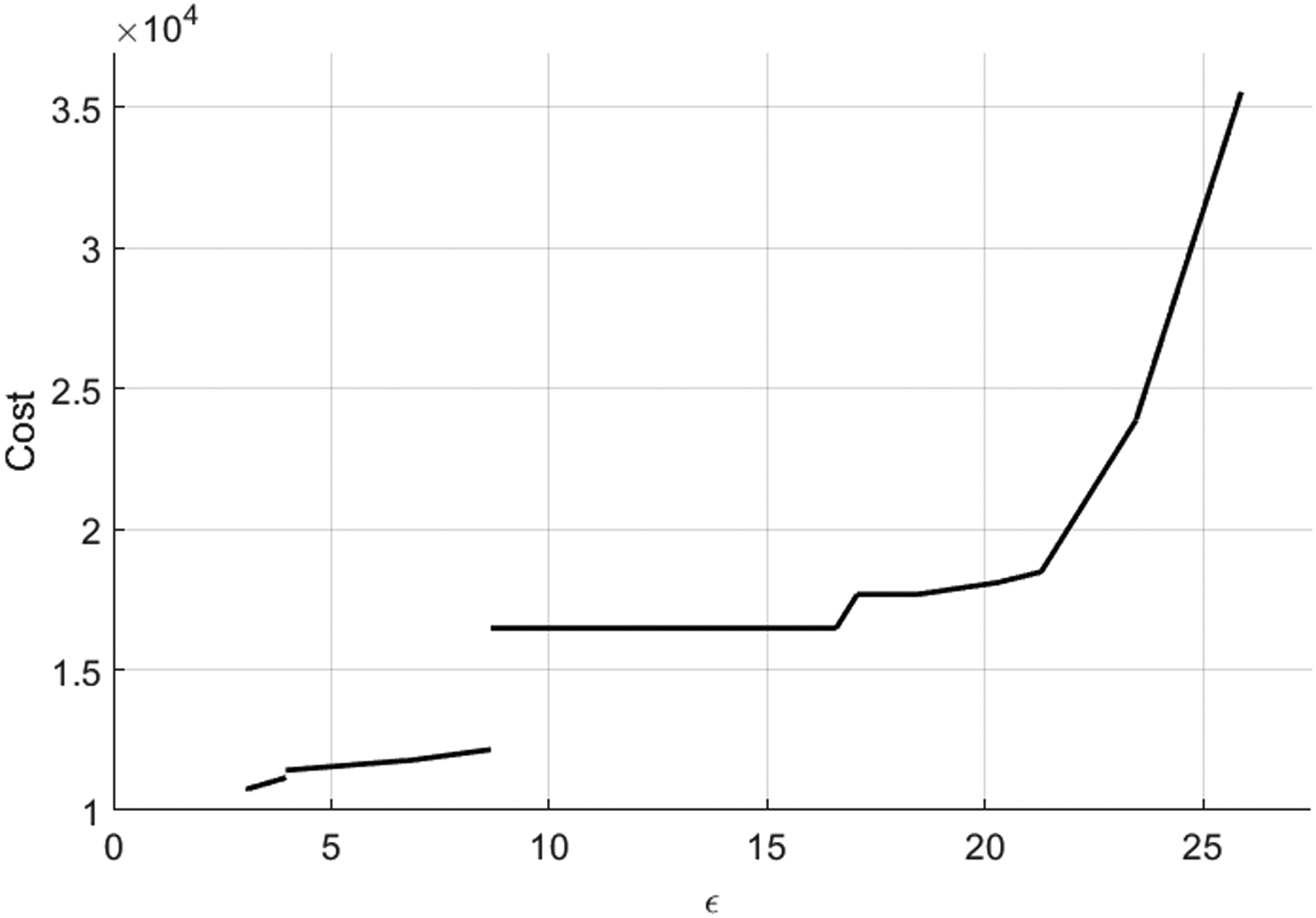
The solution of Problem (7) using the proposed multiparametric programming-based strategy for multiobjective optimization.

Table 4:

Optimal solution and Critical Region definition of Problem (7).

Critical Region	Definition	Optimal Binary Solution	Objective Function
CR1	2.800 ≤ ∊ ≤ 3.044	y = [0 0 0 1 0 0 1]T	f1 = 272.6∊ + 9, 930.7 f2 = ∊
CR2	3.044 ≤ ∊ ≤ 3.080	y = [0 0 0 1 0 0 1]T	f1 = 10,671 f2 = 3.080
CR3	3.080 ≤ ∊ ≤ 3.960	y = [0 0 0 1 0 0 1]T	f1 = 454.4∊ + 9, 360.8 f2 = ∊
CR4	3.960 ≤ ∊ ≤ 6.660	y = [0 0 0 1 0 1 1]T	f1 = 124.63∊ + 10, 931 f2 = ∊
CR5	6.660 ≤ ∊ ≤ 6.735	y = [0 0 0 1 0 1 1]T	f1 = 11, 761 f2 = 6.735
CR6	6.735 ≤ ∊ ≤ 8.660	y = [0 0 0 1 0 1 1]T	f1 = 207.8∊ + 10, 361 f2 = ∊
CR7	8.660 ≤ ∊ ≤ 16.580	y = [1 0 0 0 1 1 1]T	f1 = 16, 478 f2 = 16.580
CR8	16.580 ≤ ∊ ≤ 17.065	y = [1 0 0 0 1 1 1]T	f1 = 2, 476.8∊ − 24.589 f2 = ∊
CR9	17.065 ≤ ∊ ≤ 18.454	y = [1 0 0 1 1 1 1]T	f1 = 17, 678 f2 = ∊
CR10	18.454 ≤ ∊ ≤ 20.196	y = [1 0 0 1 1 1 1]T	f1 = 229.6∊ + 13, 342 f2 = ∊
CR11	20.196 ≤ ∊ ≤ 20.240	y = [1 0 0 1 1 1 1]T	f1 = 18, 078 f2 = ∊
CR12	20.240 ≤ ∊ ≤ 21.283	y = [1 0 0 1 1 1 1]T	f1 = 382.8∊ + 10, 332 f2 = ∊
CR13	21.283 ≤ ∊ ≤ 23.461	y = [1 0 0 1 1 1 1]T	f1 = 2,476.8∊ − 34, 236 f2 = ∊
CR14	23.461 ≤ ∊ ≤ 25.872	y = [1 0 0 1 1 1 1]T	f1 = 4, 828.6∊ − 89, 389 f2 = ∊

We observe that the Pareto front of this case study consists of 14 piecewise linear segments, described by the corresponding critical regions and optimal multiparametric expressions as shown in Table 4. The results demonstrate that due to the multiobjective nature of the problem, an increase in the mechanical strength of the final product generally leads to an overall production cost. However, this is not always the case such as in critical regions 2, 5, 7, 9, 11 of the optimal solution which generates a Weakly Pareto set. Note that the changes in the optimal binary combinations result in jumps in the optimal objective function values, resulting in an overall disjoint and nonconvex Pareto front. Finally the computational cost of deriving the optimal solution is 295.6s, showing that the approach can be utilized with low computational effort.

5. Computational Studies

A set of multiobjective mixed-integer linear optimization problems with different dimensionalities was solved to investigate the capabilities of the proposed approach. The randomly generated problems have the general mathematical form of Problem (1). For each dimensionality a set of 3 different problem instances have been generated and Table 5 presents the computational results from the studied problems, where C denotes the total number of continuous variables of the multiobjective mixed-integer linear optimization problem instances, B denotes the total number of binary variables of the multiobjective problem instances, CR Aver. denotes the average number of critical regions in each solution, and CPU Aver. denotes the average and CPU SD denotes the standard deviation of the total computational time required for the solution of each set of problems with the same dimensionality. All the problems are solved to global optimality as the underlying mpMILP algorithm provides the exact solution with zero optimality gap.

Table 5:

Computational results of the presented multiobjective optimization approach for the randomly generated multiobjective mixed-integer linear optimization problems.

Problem	Objectives	C	B	CR Aver.	CPU Aver. (s)	CPU SD
MIMOO_01	2	6	1	4.3333	0.1659	0.1225
MIMOO_02	4	2	1	7.6667	0.5842	0.4614
MIMOO_03	6	2	1	69.6667	4.5770	2.9930
MIMOO_04	8	2	1	156.3333	13.1499	10.1948
MIMOO_05	2	8	1	3.0000	0.2936	0.1198
MIMOO_06	2	12	1	9.6667	0.6607	0.0923
MIMOO_07	2	16	1	11.6667	0.5713	0.4907
MIMOO_08	2	2	6	3.0000	2.3120	3.4712
MIMOO_09	2	2	12	8.3333	22.1538	32.9812
MIMOO_10	2	2	15	14.3333	400.8611	683.7804
MIMOO_11	2	30	15	26.3333	681.1281	1040.6784
MIMOO_12	2	50	10	74.000	72.4062	53.2411
MIMOO_13	2	100	5	161.3333	119.2052	17.9729
MIMOO_14	3	10	10	6.0000	14.0043	19.3529
MIMOO_15	2	3	20	12.6667	17.0996	26.6071

The computations were carried out on a machine with an Intel Core i5 at 3.4 GHz and 8 GB of RAM, MATLAB R2019a, and IBM ILOG CPLEX Optimization Studio 12.6.3. The test problems presented in Table 5 and Figures 5 and 6 can be found in http://parametric.tamu.edu/POP/ website as ‘MIMOO’.

Figure 5:

Computational performance of the presented multiobjective optimization approach for randomly generated multiobjective mixed-integer linear optimization problems with increasing number of continuous variables (the number of binary variables is fixed to 2).

Figure 6:

Computational performance of the presented multiobjective optimization approach for randomly generated multiobjective mixed-integer linear optimization problems with increasing number of binary variables (the number of continuous variables is fixed to 2).

As it can be observed from Table 5 and the two plots (Figures 5 and 6), the computational requirements for the solution of multibojective optimization problems are increasing for higher dimensional problems. It can be concluded that the computational time is more sensitive to the number of objectives than the number of variables in multiobjective mixed-integer linear optimization problems. The reason for this is that every objective function corresponds to an added parameter in the reformulated mpMILP problem, therefore this significantly increases the complexity of the corresponding multiparametric programming problem. In summary, the computational performance of the proposed approach is directly associated with the performance of the multiparametric programming algorithm used, which scales with the number of variables, objectives, and parameters of the problem.⁴⁹

Additionally, as multiobjective problems with 2 or 3 objectives are frequently encountered, we investigated how the proposed strategy performs in problems with such objective dimensionality. For instance in engineering and supply chain applications, the overall cost must be simultaneously minimized along with the CO₂ emissions,^7,35,39 the maximization of target products, the minimization of unwanted materials, and the minimization of greenhouse emissions⁵² must be achieved or economic, environmental and market maturity criteria¹ must be considered. Further computational experiments were carried out to assess the complexity and the applicability of the presented multiobjective approach with respect to the continuous and binary variables. For each problem dimensionality presented in Figures 5 and 6, a set of 3 instances was generated and solved. It can be observed that with the increasing number of continuous and binary variables, the computational complexity is amplified, which is due to the larger size of the mpLP problem that needs to be solved at each node of the mpB&B tree, and due to the increased number of mpB&B nodes due to the higher number of binary variables.

6. Conclusion

In this work, a methodology for the exact and explicit solution of multiobjective mixed-integer linear optimization problems was presented. The proposed approach incorporates the reformulation of the multiobjective optimization problem into a single objective multi-parametric programming problem, through the ϵ-constraint method. As a result, the explicit description of the potentially discontinuous and nonconvex Pareto front can be achieved, by treating the ϵ vector as a vector of uncertain parameters. Hence, the computational effort to generate Pareto optimal solutions is drastically reduced compared to iterative approaches, and the decision maker can readily select an optimal solution. Furthermore, due to the explicit structure of the optimal solution, weakly Pareto optimal solutions can be identified. The proposed strategy was applied to an illustrative numerical example and to a process and product design process, successfully minimizing the production cost and maximizing the mechanical strength of the desired product. Finally, a set of randomly generated numerical case studies of varying dimensionality was solved. The results indicated that the computational complexity is amplified with the increasing number of variables and objectives, due to more challenging continuous multiparametric linear programming problems that needed to be solved.

Appendix

Simultaneous Product and Process Design Model

The optimization problem of the case study in Section 4 is formulated bellow.

min	[Cost, – Mechanical Strength]
Fi,in, Fi,out, Rk, Xi, Pi, Ti
$AS,LS,{\widehat{P}}_{4,l},{\widehat{P}}_{5,m}{Y}_i,N_l,W_m$
s.t.	F1,out − 0.7F1,in = 0
	F2,out − 0.85F2,in = 0
	F3,out − 0.65F3,in = 0
	F4,out − 0.85F4,in = 0
	F5,out − 0.99F5,in = 0
	F6,out − 0.97F6,in = 0
	F7,out – 0.9F7,in = 0
	R2 − 0.4F4,out = 0
	R2 + LS − F4,in = 0
	R1 − 0.2F5,out = 0
	R1 + AS + F1,out + F2,out + F3,out − F5,in = 0
	F6,in + F7,in − F4,out − F5,out = 0
	X4 − 20Y4 ≤ 0
	X5 − 150Y5 ≤ 0
	−X6 − X7 + 2.8 ≤ 0
	−X6 − 25Y6 ≤ 0
	X7 − 7Y7 ≤ 0
	X6 − 0.95(X4 + X5) ≤ 0
	X7 − 0.8(X4 + X5) ≤ 0
	−F6,out − F7,out + 30 ≤ 0
	Fi,in − 1000Yi ≤ 0, ∀i
	20Y4 ≤ T4< 1000Y4
	1 + Y4 ≤ P4 ≤ 5Y4 + 1
	20Y5 ≤ T5 ≤ 200Y5
	1 + 30Y5 ≤ P5 ≤ 150Y5 + 1
	$X_4-1.833{\widehat{P}}_{4,1}-0.917{\widehat{P}}_{4,2}-0.550{\widehat{P}}_{4,3}+1.723N_1-$
	+0.138N2 – 1.650N3 + 10−5T4 + 1500Y4 − 1500 ≤ 0
	$X_5-1.987{\widehat{P}}_{5,1}-0.993{\widehat{P}}_{5,2}-0.436{\widehat{P}}_{5,3}-0.213{\widehat{P}}_{5,4}-0.085{\widehat{P}}_{5,5}-$
	$-0.043{\widehat{P}}_{5,6}-1.877W_1-0.149W_2-2.682W_3-4.768W_4-$
	+7.450W5 – 9.54W6 − 10−5T5 + 1500Y5 − 1500 ≤ 0
	$P_4-{\widehat{P}}_{4,1}-{\widehat{P}}_{4,2}-{\widehat{P}}_{4,3}=0$
	$P_5-{\widehat{P}}_{5,1}-{\widehat{P}}_{5,2}-{\widehat{P}}_{5,3}-{\widehat{P}}_{5,4}-{\widehat{P}}_{5,5}-{\widehat{P}}_{5,6}=0$
	N1 + N2 + N3 = 1
	W1 + W2 + W3 + W4 + W5 + W6 = 1
	Fi,in ≥ 0,∀i
	Fi,out ≥ 0,∀i
	Rk ≥ 0, ∀k
	Xi ≥ 0, ∀i
	Pi ≥ 0,∀i
	Ti ≥ 0, ∀i
	AS ≥ 0,∀i
	LS ≥ 0,∀i
	Yi ∈{0,1}
	Nl ∈ {0,1}
	Wm ∈ {0,1}
Cost = 0.3F1,in + 150F2,in + 160F3,in + 700F6,in + 200F7,in + 200P4 + 10T4 + 200P5 + 15T5 + 100Y1 + 1500Y2 + 1200Y3 + 800Y4 + 1200Y5 + 1000Y6 + 800Y7 + 5AS + 50LS − 400
Mechanical Strength = X6 + X7

where F_i,in and F_i,out are the inlet and outlet flowrates at process i, R_k is the flowrate of the k^th recycle stream, and LS and AS are the aqueuous and nonaqueous solvent flowrates. The mechanical strength of the composite product out of process i is denoted with X_i, while with P_i and T_i the process pressure and temperature are respectively defined. Finally, the continuous variables ${\widehat{P}}_{4,l}{\widehat{P}}_{5,m}$, and the binaries N_l, and W_m, are introduced from the linearization of the two nonlinear constraints from Papalexandri and Dimkou³⁴.

References

- (1).Li L; Liu P; Li Z; Wang X A multi-objective optimization approach for selection of energy storage systems. Comput. Chem. Eng 2018, 115, 213–225. [Google Scholar]
- (2).Marler RT; Arora JS Survey of multi-objective optimization methods for engineering. Struct. Multidiscipl. Optim 2004, 26, 369–395. [Google Scholar]
- (3).Zamboni A; Bezzo F; Shah N Spatially Explicit Static Model for the Strategic Design of Future Bioethanol Production Systems. 2. Multi-Objective Environmental Optimization. Energy Fuels 2009, 23, 5134–5143. [Google Scholar]
- (4).Zhou T; Song Z; Zhang X; Gani R; Sundmacher K Optimal solvent design for extractive distillation processes: A multiobjective optimization-based hierarchical framework. Ind. Eng. Chem. Res 2019, 58, 5777–5786. [Google Scholar]
- (5).Öztürk A; Türkay M Bicriteria optimization approach to analyze incorporation of biofuel and carbon capture technologies. AIChE J. 2016, 62, 3473–3483. [Google Scholar]
- (6).Di Martino M; Avraamidou S; Cook J; Pistikopoulos EN An optimization framework for the design of reverse osmosis desalination plants under food-energy-water nexus considerations. Desalination 2021, 503, 114937. [Google Scholar]
- (7).Beykal B; Boukouvala F; Floudas CA; Pistikopoulos EN Optimal design of energy systems using constrained grey-box multi-objective optimization. Comput. Chem. Eng 2018, 116, 488–502. [DOI] [PMC free article] [PubMed] [Google Scholar]
- (8).Du Y; Xie L; Liu J; Wang Y; Xu Y; Wang S Multi-objective optimization of reverse osmosis networks by lexicographic optimization and augmented epsilon constraint method. Desalination 2014, 333, 66–81. [Google Scholar]
- (9).Avraamidou S; Baratsas SG; Tian Y; Pistikopoulos EN Circular Economy-A challenge and an opportunity for Process Systems Engineering. Comput. Chem. Eng 2020, 133, 106629. [Google Scholar]
- (10).You F; Tao L; Graziano DJ; Snyder SW Optimal design of sustainable cellulosic biofuel supply chains: Multiobjective optimization coupled with life cycle assessment and input–output analysis. AIChE J. 2012, 58, 1157–1180. [Google Scholar]
- (11).Rasmi SAB; Kazan C; Türkay M A multi-criteria decision analysis to include environmental, social, and cultural issues in the sustainable aggregate production plans. Comput. Ind. Eng 2019, 132, 348–360. [Google Scholar]
- (12).Pardalos PM; Žilinskas A; Žilinskas J Non-convex multi-objective optimization; Springer, 2017. [Google Scholar]
- (13).Pascual-González J; Jiménez-Esteller L; Guillén-Gosálbez G; Siirola JJ; Grossmann IE Macro-economic multi-objective input–output model for minimizing CO2 emissions: Application to the U.S. economy. AIChE J. 2016, 62, 3639–3656. [Google Scholar]
- (14).Miettinen K Nonlinear multiobjective optimization; Springer Science & Business Media, 1999; Vol. 12. [Google Scholar]
- (15).Miettinen K In Multiobjective Optimization: Interactive and Evolutionary Approaches; Branke J, Deb K, Miettinen K, Słowiński R, Eds.; Springer Berlin Heidelberg: Berlin, Heidelberg, 2008; pp 1–26. [Google Scholar]
- (16).Ruzika S; Wiecek MM Approximation Methods in Multiobjective Programming. J. Optim. Theory Appl 2005, 126, 473–501. [Google Scholar]
- (17).Deb K; Saxena DK On finding pareto-optimal solutions through dimensionality reduction for certain large-dimensional multi-objective optimization problems. Kangal report 2005, 2005011. [Google Scholar]
- (18).Burachik RS; Kaya CY; Rizvi MM Algorithms for generating pareto fronts of multi-objective integer and mixed-integer programming problems. arXiv preprint arXiv:1903.07041 2019, [Google Scholar]
- (19).Mavrotas G Effective implementation of the ε-constraint method in Multi-objective Mathematical Programming problems. Appl. Math. Comput 2009, 213, 455–465. [Google Scholar]
- (20).Guillén-Gosálbez G A novel MILP-based objective reduction method for multiobjective optimization: Application to environmental problems. Comput. Chem. Eng 2011, 35, 1469–1477. [Google Scholar]
- (21).Bitran GR Linear multiple objective programs with zero–one variables. Math. Program 1977, 13, 121–139. [Google Scholar]
- (22).Bitran GR Theory and algorithms for linear multiple objective programs with zero–one variables. Math. Program 1979, 17, 362–390. [Google Scholar]
- (23).Parragh SN; Tricoire F Branch-and-bound for bi-objective integer programming. INFORMS J. Comput 2019, 31, 805–822. [Google Scholar]
- (24).Mavrotas G; Diakoulaki D A branch and bound algorithm for mixed zero-one multiple objective linear programming. Eur. J. Oper. Res 1998, 107, 530–541. [Google Scholar]
- (25).Belotti P; Soylu B; Wiecek MM A branch-and-bound algorithm for biobjective mixed-integer programs. Optimization Online 2013, [Google Scholar]
- (26).Boland N; Charkhgard H; Savelsbergh M A criterion space search algorithm for biobjective mixed integer programming: The triangle splitting method. INFORMS J. Comput 2015, 27, 597–618. [Google Scholar]
- (27).Soylu B; Yıldız GB An exact algorithm for biobjective mixed integer linear programming problems. Comput. Oper. Res 2016, 72, 204–213. [Google Scholar]
- (28).Fattahi A; Türkay M A one direction search method to find the exact nondominated frontier of biobjective mixed-binary linear programming problems. Eur. J. Oper. Res 2018, 266, 415–425. [Google Scholar]
- (29).Rasmi SAB; Fattahi A; Türkay M SASS: slicing with adaptive steps search method for finding the non-dominated points of tri-objective mixed-integer linear programming problems. Ann. Oper. Res 2019, 1–36. [Google Scholar]
- (30).Mavrotas G; Florios K An improved version of the augmented ε-constraint method (AUGMECON2) for finding the exact pareto set in multi-objective integer programming problems. Appl. Math. Comput 2013, 219, 9652–9669. [Google Scholar]
- (31).Borndörfer R; Schenker S; Skutella M; Strunk T PolySCIP. International Congress on Mathematical Software. 2016; pp 259–264. [Google Scholar]
- (32).Rasmi SAB; Türkay M GoNDEF: an exact method to generate all non-dominated points of multi-objective mixed-integer linear programs. Optim. Eng 2019, 20, 89–117. [Google Scholar]
- (33).Pappas I; Kenefake D; Burnak B; Avraamidou S; Ganesh HS; Katz J; Diangelakis NA; Pistikopoulos EN Multiparametric Programming in Process Systems Engineering: Recent Developments and Path Forward. Front. Chem. Eng 2021, 2. [Google Scholar]
- (34).Papalexandri KP; Dimkou TI A Parametric Mixed-Integer Optimization Algorithm for Multiobjective Engineering Problems Involving Discrete Decisions. Ind. Eng. Chem. Res 1998, 37, 1866–1882. [Google Scholar]
- (35).Hugo A; Ciumei C; Buxton A; Pistikopoulos EN Environmental impact minimization through material substitution: A multi-objective optimization approach. Green Chem. 2004, 6, 407–417. [Google Scholar]
- (36).Dua P; Doyle FJ; Pistikopoulos EN Multi-objective blood glucose control for type 1 diabetes. Med. Biol. Eng. Comput 2009, 47, 343–352. [DOI] [PubMed] [Google Scholar]
- (37).Bemporad A; de la Peña DM Multiobjective model predictive control. Automatica 2009, 45, 2823–2830. [Google Scholar]
- (38).Oberdieck R; Pistikopoulos EN Multi-objective optimization with convex quadratic cost functions: A multi-parametric programming approach. Comput. Chem. Eng 2016, 85, 36–39. [Google Scholar]
- (39).Charitopoulos VM; Dua V A unified framework for model-based multi-objective linear process and energy optimisation under uncertainty. Appl. Energy 2017, 186, 539–548. [Google Scholar]
- (40).Acevedo J; Pistikopoulos EN A Multiparametric Programming Approach for Linear Process Engineering Problems under Uncertainty. Ind. Eng. Chem. Res 1997, 36, 717–728. [Google Scholar]
- (41).Acevedo J; Pistikopoulos EN An algorithm for multiparametric mixed-integer linear programming problems. Oper. Res. Lett 1999, 24, 139–148. [Google Scholar]
- (42).Pertsinidis A; Grossmann IE; McRae GJ Parametric optimization of MILP programs and a framework for the parametric optimization of MINLPs. Comput. Chem. Eng 1998, 22, S205–S212. [Google Scholar]
- (43).Dua V; Pistikopoulos EN An algorithm for the solution of multiparametric mixed integer linear programming problems. Ann. Oper. Res 2000, 99, 123–139. [Google Scholar]
- (44).Faísca NP; Kosmidis VD; Rustem B; Pistikopoulos EN Global optimization of multi-parametric MILP problems. J. Glob. Optim 2009, 45, 131–151. [Google Scholar]
- (45).Mitsos A; Barton PI Parametric mixed-integer 0–1 linear programming: The general case for a single parameter. Eur. J. Oper. Res 2009, 194, 663–686. [Google Scholar]
- (46).Oberdieck R; Wittmann-Hohlbein M; Pistikopoulos EN A branch and bound method for the solution of multiparametric mixed integer linear programming problems. J. Glob. Optim 2014, 59, 527–543. [Google Scholar]
- (47).Li Z; Ierapetritou MG A New Methodology for the General Multiparametric Mixed-Integer Linear Programming (MILP) Problems. Ind. Eng. Chem. Res 2007, 46, 5141–5151. [Google Scholar]
- (48).Charitopoulos VM; Papageorgiou LG; Dua V Multi-parametric mixed integer linear programming under global uncertainty. Comput. Chem. Eng 2018, 116, 279–295. [Google Scholar]
- (49).Oberdieck R; Diangelakis NA; Papathanasiou MM; Nascu I; Pistikopoulos EN POP–Parametric OPtimization Toolbox. Ind. Eng. Chem. Res 2016, 55, 8979–8991. [Google Scholar]
- (50).Katz J; Pappas I; Avraamidou S; Pistikopoulos EN Integrating Deep Learning Models and Multiparametric Programming. Comput. Chem. Eng 2020, 136, 106801. [Google Scholar]
- (51).Pappas I; Diangelakis NA; Pistikopoulos EN The exact solution of multiparametric quadratically constrained quadratic programming problems. J. Glob. Optim 2021, 79, 59–85. [Google Scholar]
- (52).Tarafder A; Rangaiah G; Ray AK Multiobjective optimization of an industrial styrene monomer manufacturing process. Chem. Eng. Sci 2005, 60, 347–363. [Google Scholar]