

Abstract
Habitat‐selection analyses allow researchers to link animals to their environment via habitat‐selection or step‐selection functions, and are commonly used to address questions related to wildlife management and conservation efforts. Habitat‐selection analyses that incorporate movement characteristics, referred to as integrated step‐selection analyses, are particularly appealing because they allow modelling of both movement and habitat‐selection processes.
Despite their popularity, many users struggle with interpreting parameters in habitat‐selection and step‐selection functions. Integrated step‐selection analyses also require several additional steps to translate model parameters into a full‐fledged movement model, and the mathematics supporting this approach can be challenging for many to understand.
Using simple examples, we demonstrate how weighted distribution theory and the inhomogeneous Poisson point process can facilitate parameter interpretation in habitat‐selection analyses. Furthermore, we provide a ‘how to’ guide illustrating the steps required to implement integrated step‐selection analyses using the amt package
By providing clear examples with open‐source code, we hope to make habitat‐selection analyses more understandable and accessible to end users.
Keywords: habitat‐selection function, inhomogeneous Poisson point process, integrated step‐selection analysis, intensity function, resource‐selection function, relative selection strength, step‐selection function, telemetry
Habitat‐selection analyses allow researchers to link animals to their environment in support of wildlife management and conservation efforts. We provide a ‘how to' guide for correctly interpreting parameters in habitat‐ and step‐selection functions and for implementing integrated step‐selection analyses using the amt package for program R.
1. INTRODUCTION
New technologies (e.g. improved Global Positioning System [GPS] collars) and advances in remote sensing have made it possible to collect animal location data on unprecedented spatial and temporal scales (Kays et al., 2015; Robinson et al., 2020), which in turn has fuelled the development of new methods for modelling animal movement and for linking individuals to their environments (Guisan et al., 2017; Hooten et al., 2017). Two of the most popular approaches for analysing telemetry data, habitat‐selection functions (HSFs; Box 1) and step‐selection functions (SSFs), compare environmental covariates at locations visited by an animal (‘used locations’) to environmental covariates at a set of locations assumed available to the animal (‘available locations’) using logistic and conditional logistic regression respectively (Boyce & McDonald, 1999; Fortin et al., 2005; Thurfjell et al., 2014). These methods are widely available in most statistical software packages, and thus, they provide a robust and easy‐to‐implement framework for analysing habitat‐selection patterns. Note, here and throughout, we use the term habitat‐selection function rather than the traditional resource‐selection function to highlight our broader interest in modelling the effects of a diverse set of environmental variables (e.g. those capturing risks and environmental conditions in addition to resources). Habitat‐selection functions are used to identify habitat features that are preferentially used or avoided by a species, and thus, to infer ecological needs and limitations, generate expected distribution maps and inform demographic projections across space and time in support of species and landscape management (Boyce & McDonald, 1999; Matthiopoulos et al., 2015, 2019). Step‐selection functions are further used to identify fine‐scale behavioural interactions between animals and their biotic and abiotic environment (e.g. Dickie et al., 2020). Despite their popularity, our collective experience has been that many users struggle to interpret parameters in HSFs and SSFs. Furthermore, it seems that papers attempting to address this issue have had limited success, and in some aspects may have increased confusion (see e.g. Avgar et al., 2017; Chamaille‐Jammes, 2019; Johnson et al., 2006; Keating & Cherry, 2004; Lele et al., 2013).
BOX 1. Overview of habitat‐selection functions (HSFs).
Habitat‐selection functions (HSFs; historically referred to as ‘resource‐selection functions’; Boyce & McDonald, 1999) provide a framework for linking locations of individual animals to important features of their environment (i.e. resources, risks and environmental conditions).
Exponential HSFs, the most common HSF in the literature, take the form ; where the are environmental predictors associated with location , and the are parameters to be estimated.
Parameters in HSFs are typically estimated using logistic regression, but with use‐availability data rather than presence–absence data. The use of logistic regression to model use‐availability data has created significant confusion in the literature.
Inhomogeneous Poisson Point process (IPP) Models and Weighted Distribution Theory provide suitable frameworks for interpreting HSF parameters estimated using logistic regression (Aarts et al., 2012; Fithian & Hastie, 2013; Matthiopoulos, Fieberg, & Aarts, 2020; Warton & Shepherd, 2010). These frameworks require that users include sufficient available points to ensure parameter estimates converge to stable values (Figure 2; Warton & Shepherd, 2010). In addition, available points should be assigned large weights when fitting logistic regression models (Fithian & Hastie, 2013).
For continuous predictors, , exponentiated HSF coefficients, , quantify the relative intensity of use of locations that differ by 1 unit of , but are otherwise equivalent (i.e. they are assumed to be equally available and to have equivalent values for all other predictor variables).
For categorical predictors, , exponentiated HSF coefficients, , quantify the relative intensity of use of locations in category relative to locations in a reference category, assuming both categories are equally available and that the locations do not differ with respect to other predictors.
Here, we highlight how point process models and weighted distribution theory provide simple and effective frameworks for interpreting regression parameters in habitat‐selection and step‐selection functions. In the sections that follow, we begin by reviewing recent research connecting habitat‐selection functions to point process models and weighted distribution theory. Using these connections, we demonstrate correct interpretation of parameters using simple examples of models fit to GPS locations of fisher Pekania pennanti from upstate New York (LaPoint et al., 2013a, 2013b). We then provide a short review of step‐selection functions, including their history and methods for parameter estimation. Step‐selection analyses (Box 2) are particularly appealing because: (a) they provide an objective method for defining habitat availability in terms of movement constraints; (b) they relax the assumption that locations are statistically independent; and (c) by including movement characteristics (e.g. functions of step length and turn angle) as predictors, they provide a means to model both movement and habitat‐selection processes (termed an integrated step‐selection analysis by Avgar et al., 2016). Recognizing that many may find the mathematics supporting integrated step‐selection analyses intimidating, we aim to provide a ‘how to’ guide demonstrating the steps required to implement the approach using the amt package (Signer et al., 2019). This demonstration is expanded upon using coded examples in the Supporting Information, which we encourage the reader to explore. We end with a short discussion highlighting challenges related to statistical dependencies and model transferability.
BOX 2. Overview of step‐selection analyses.
Step‐selection analyses model transitions or ‘steps’ connecting sequential locations in geographical space using a selection‐free movement kernel, , multiplied by a habitat‐selection kernel, (Avgar et al., 2016; Forester et al., 2009). Available locations are dynamic in space and time, with availability determined by the previous location and the animal's selection‐free movement kernel.
The selection‐free movement kernel describes how the animal would move in homogeneous habitat or in the absence of habitat selection.
-
Movement and habitat‐selection parameters are typically estimated in a multi‐step process:
preliminary movement parameters are estimated using observed step lengths and turn angles;
time‐dependent availability distributions are generated by simulating potential movements from the previously observed location;
habitat‐selection parameters are estimated using conditional logistic regression, with strata formed by combining time‐dependent used and available locations;
if movement characteristics (e.g. log step length, cosine of the turn angle) are included in the model, parameters associated with these characteristics can be used to update the preliminary movement parameters from step 1. Including movement characteristics in the model can reduce bias in the habitat‐selection parameters (Forester et al., 2009) and improve estimates of movement parameters (Avgar et al., 2016).
Interactions between movement characteristics (e.g. log step length, cosine of the turn angle) and environmental covariates may be included in the conditional logistic regression model to allow the movement kernel to depend on the environment (Avgar et al., 2016; Duchesne et al., 2015).
Habitat‐selection parameters can be interpreted in terms of relative intensities of use, assuming locations are equally available and differing in terms of a single habitat covariate. However, parameters that describe habitat‐selection at local and macro scales may differ, and extra steps may be required to translate movement dynamics captured by integrated step‐selection analyses to the courser scales typically modelled with HSFs (e.g. Potts, Bastille‐Rousseau, et al., 2014; Potts, Mokross, et al., 2014; Potts & Schlägel, 2020; Signer et al., 2017).
2. HABITAT‐SELECTION FUNCTIONS
2.1. Logistic regression
Much of the confusion surrounding the interpretation of parameters in habitat‐selection functions can be attributed to the use of logistic regression to model use‐availability data (Keating & Cherry, 2004). Logistic regression is most easily understood as a model for binary random variables that can take on one of two values (0 or 1) with probability that depends on one or more explanatory variables (Hosmer, Lemeshow, & Sturdivant, 2013).
Consider, for example, a study designed to infer how various environmental characteristics influence whether a habitat patch (e.g. a contiguous area of forest) will be used by one or more animals. In this case, we may randomly select habitat patches and monitor them to determine if they are used () or not () for . Logistic regression allows us to model the probability that each patch will be used, , as a logit‐linear function of patch‐level predictors () and regression parameters ():
After having fit a model, we can exponentiate the regression coefficients, for , to quantify how the odds of patch being used, , change as we increase the jth predictor by 1 unit while holding all other predictors constant. We can also use the inverse‐logit transformation (Equation 1) to estimate the probability that patch will be used, given its set of spatial predictors:
| (1) |
The logit transformation ensures that will be constrained between 0 and 1 for all values of the predictor variables.
Contrast this approach with how logistic regression is used to study habitat selection. In a typical habitat‐selection study, logistic regression models are fit to separate samples of used and available sample units, usually points; these groups are not mutually exclusive (i.e. available habitat may also be used). In this case, is no longer a Bernoulli random variable since depends on the ratio of used to available points (which is under control of the analyst). That is, the probability that a location will be a ‘used point’ decreases with the number of user‐generated ‘available’ locations. Furthermore, despite the fact that most analyses of telemetry data quantify environmental covariates in discrete space (i.e. pixels in a raster), the sampling itself is point level and in continuous space. Thus, it is perhaps not surprising that there has been considerable confusion and controversy surrounding the use of logistic regression with use‐availability data (e.g. Chamaille‐Jammes, 2019; Johnson et al., 2006; Keating & Cherry, 2004).
Various arguments have been constructed to justify the use of logistic regression when analysing use‐availability data (Aarts et al., 2008; Johnson et al., 2006; Manly et al., 2002), but a significant breakthrough came when Warton and Shepherd (2010) made a connection between logistic regression and a spatial inhomogeneous Poisson point process (IPP). A spatial IPP is a model for random locations in space, where the expected spatial density of the locations depends on spatial predictors (see next Section 2.2). Warton and Shepherd (2010) showed that as the number of available points is increased towards infinity, the slope parameters in logistic regression models will converge to the slope parameters in an IPP model. Interestingly, several other popular approaches for analysing species distribution data, including MaxEnt (Elith et al., 2011; Phillips & Dudík, 2008), weighted distribution theory with an exponential form (Lele & Keim, 2006) and resource utilization functions (Millspaugh et al., 2006), have been shown to be equivalent to fitting a spatial IPP model (Aarts et al., 2012; Fithian & Hastie, 2013; Hooten et al., 2013; Renner et al., 2015; Warton & Shepherd, 2010).
Instead of focusing on , as is typical in applications to presence–absence data, logistic regression applied to use‐availability data should simply be viewed as a convenient tool for estimating coefficients in a habitat‐selection function, (Boyce & McDonald, 1999; Boyce et al., 2002), where we have written to highlight that the predictors correspond to measurements at specific point locations in geographical space, . As we will see in the next section, this expression is equivalent to the intensity function of an IPP model but with the intercept (the log of the baseline intensity) removed; the baseline intensity gives the expected density of points when all covariates are 0. Because habitat‐selection functions do not include this baseline intensity, they are said to measure ‘relative probabilities of use’, or alternatively, said to be ‘proportional to the probability of use’ (Manly et al., 2002). Although the term probability of use sounds appealing, probability in continuous space can only be assigned to areas, not points. Furthermore, although probability of use is easily defined for discrete sample units (e.g. grid cells), these probabilities should increase with the size of the spatial unit and also with the study duration (Lele & Keim, 2006; Lele et al., 2013). Thus, with telemetry studies, it seems more natural to model spatial (or spatio‐temporal) intensity functions or rates of use in continuous space (and time). Subsequently, ‘probabilities of use’ can be determined by integrating these intensity functions over whatever spatial (and temporal) unit is deemed appropriate. Point process models allow us to do just that.
2.2. Inhomogeneous Poisson point process model
The IPP model provides a simple framework for modelling the density of points in space as a loglinear function of spatial predictors through a spatially varying intensity function, :
| (2) |
where s is a location in geographical space, and are spatial predictors associated with location . The intercept, , determines the log density of points (within a small homogeneous area around ) when all are 0, and the slopes, , describe the effect of spatial covariates on the log density of points in space. The IPP model can be understood by listing its key features and assumptions, namely:
The number of points in an area , , is a Poisson random variable with mean (the spatial integral of over ).
Locations are independent (any clustering can be explained by spatial covariates).
If all available spatial predictors are measured only at a coarse scale (e.g. at a set of gridded or rasterized cells), then fitting the IPP model is equivalent to fitting a Poisson regression model (Aarts et al., 2012). Specifically, one may treat the counts, , in discrete spatial units (), as a set of independent Poisson random variables with means = where is given by Equation (2) and is the area of unit . Note that . Thus, the log‐link used in Poisson regression implies the area, , should be included as an offset (a predictor variable with regression coefficient fixed at a value of 1).
When spatial predictors are available at the point level, as will be the case whenever constructing ‘distance to’ predictors (e.g. distance to nearest road, water source, etc.), it will be advantageous to model the locations in continuous space. In telemetry studies, the density of points will be determined by the frequency and duration of data collection. Thus, will not be of biological interest, and it will be appropriate to focus efforts on estimating and interpreting the slope coefficients, , which determine relationships between the spatial covariates and the relative density of locations throughout the study area (Fithian & Hastie, 2013). As is the case with linear and generalized linear models (e.g. Poisson regression), we can estimate parameters using maximum likelihood or Bayesian methods. Both approaches require writing down an expression, called the likelihood, that captures the data‐generating mechanism in terms of one or more parameters. With telemetry data, it makes sense to work with the conditional likelihood of the IPP model (Aarts et al., 2012), that is, the likelihood of the observed locations in space, conditional on there being total observed locations. The conditional likelihood is given by:
| (3) |
where the product is over the observed locations, is the intensity function evaluated at observation , and the integral in the denominator evaluates the intensity function over the spatial domain of interest (Aarts et al., 2012; Cressie, 1992). If we plug into Equation (3), will cancel from the numerator and denominator, leaving us with:
| (4) |
where is our habitat‐selection function.
The binomial likelihood associated with logistic regression differs from Equation (4), but Warton and Shepherd (2010) showed that logistic regression estimators of slope coefficients converge to the those of the IPP model as the number of available points increases towards infinity. Thus, the connection to the IPP model addresses a common question that arises when estimating habitat‐selection functions, namely, ‘how many available points do I need?’ The exact answer depends on how difficult it is to estimate the integral in the denominator of Equation (4); the recommendation we offer is to increase the number of available points until the estimated slope coefficients no longer change much. Fithian and Hastie (2013) later showed that the convergence results of Warton and Shepherd (2010) hold only if the model is correctly specified, but assigning ‘infinite weights’ to available points ensures the results hold more generally. Therefore, when fitting logistic regression or other binary response models (e.g. boosted regression trees) to use‐availability data, we also suggest assigning a large weight (say 5,000 or more) to each available location and a weight of 1 to all observed locations (larger weights can be used to verify that results are robust to this choice). For a coded example in R (R Core Team, 2019), see Section 2.4 and Supporting Information Appendix A.
2.3. Weighted distributions
Weighted distribution theory provides another way to interpret parameters in habitat‐selection functions (Johnson et al., 2008; Lele & Keim, 2006). Let:
= the frequency distribution of habitat covariates, , at locations used by our study animals.
= the frequency distribution of habitat covariates, , at locations assumed to be available to our study animals.
We can think of the habitat‐selection function, , as providing a set of weights that takes us from the distribution of available habitat to the distribution of used habitat:
| (5) |
The denominator of Equation (5) ensures that the right‐hand side integrates to 1, and thus, is a proper probability distribution; the variable here is just a dummy variable used to allow integration over the frequency distribution of our environmental covariates. Because these distributions are written in terms of the habitat covariates, , instead of geographical locations, we say that model is parameterized in environmental space () (Elith & Leathwick, 2009; Hirzel & Le Lay, 2008; Matthiopoulos, Fieberg, Aarts, Barraquand, et al., 2020).
To show that weighted distribution theory is consistent with the IPP formulation discussed above, we can rewrite Equations (5) in geographical space ():
| (6) |
where the denominator integrates over a geographical area, , that is assumed to be available to the animal and is a dummy variable for integration. Here is equivalent to the utilization distribution encountered in the literature on probabilistic estimators of animal home ranges (Signer & Fieberg, 2020; Van Winkle, 1975; Worton, 1989) and tells us how likely we are to find an individual at location in geographical space. The utilization distribution, , depends on the environmental covariates associated with location , through , and the distribution of available locations in geographical space, . When fitting HSFs, is typically assumed to be a uniform distribution within the geographical domain of availability, (e.g. the individual's home range, the population's range or the species range depending on the hierarchical level of habitat selection of interest; Johnson, 1980), with all areas within assumed to be equally available to the organism. Hence, is typically a constant, , that cancels from the numerator and denominator. Then, if we let , we end up with the conditional likelihood of the IPP model (Equation 4; Aarts et al., 2012). In summary, the IPP model and weighted distribution theory with an exponential form provide equivalent, suitable frameworks for interpreting parameters in logistic regression models fit to use‐availability data.
2.4. Interpreting parameters in habitat‐selection functions
To demonstrate how the IPP and weighted distribution theory frameworks help with interpreting parameters in fitted habitat‐selection functions, we now consider a simple example using 3,004 locations of a fisher named Lupe tracked as part of a larger telemetry study (LaPoint et al., 2013a, 2013b). These data are publicly available and have been featured in a workshop highlighting Movebank's Env‐DATA system for annotating locations with environmental covariates (Dodge et al., 2013; Fieberg, Bohrer, et al., 2018). The location data were combined with available points sampled randomly from within a minimum convex polygon (MCP) formed using Lupe's locations. The used and available locations were then transformed to a projected coordinate reference system (NAD83/Conus Albers) and annotated with environmental variables measuring human population density (Center for International Earth Science Information Network (CIESIN) Columbia University, & CIAT, Centro Internacional de Agricultura Tropical, 2005), elevation (U.S./Japan ASTER Science Team, 2009) and landcover class (Defourny et al., 2009). The original landcover data were grouped to form a variable named landuseC with the following categories: forest, grass and wet (Figure 1). We created centred (mean = 0) and scaled (SD = 1) variables labelled elevation and popden from the original elevation and population density variables. We also created an indicator variable, case_, taking on a value of 1 for all used points and 0 for all available points (later, we discuss how to choose the number of available points).
FIGURE 1.
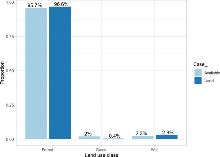
FDistribution of used and available locations among different landscape cover classes for a fisher in upstate New York (LaPoint et al., 2013a, 2013b)
For ease of interpretation, we will begin by assuming the effects of elevation, population density and landcover class are additive and linear (on the log scale; Equation 2). Later, we will discuss how we can relax these assumptions using interactions to allow the effect of covariates to depend on the value of other habitat covariates and polynomials or splines to relax the assumption of linearity. We assign a weight of 5,000 to the available locations and a weight of 1 to all observed locations (Fithian & Hastie, 2013). We can then fit a weighted logistic regression model using the glm function in R:
Lupe.dat$w <– ifelse(Lupe.dat$case_==1, 1, 5000)


HSF.Lupe <– glm(case_ ~ elevation + popden + landuseC,


 data = Lupe.dat,


 weight = w,


 family = binomial)
Before interpreting the coefficients, it is important to make sure we have included a sufficient number of available points to allow parameter estimates to converge to stable values. To evaluate parameter stability, we fit logistic regression models to datasets with increasing numbers of available points (from 1 available point per used point to 100 available points per used point; see Supporting Information Appendix A for the code). The intercept decreased as we increased the number of available points (as it is roughly proportional to the log difference between the numbers of used and available points), but the slope parameter estimates, on average, did not change much once we included at least 10 available points per used point (Figure 2). Furthermore, as expected, estimates varied less from sample to sample as we increased the number of available points. Thus, we conclude that, in this particular case, having 10 available points per used point is sufficient for interpreting the slope coefficients. The only downside to including even more available points is that it may slow down computations, which is not an issue here. Increasing the number of available points also further reduces Monte Carlo error, so we proceed with the largest sample size we explored (100 available points per used point).
FIGURE 2.
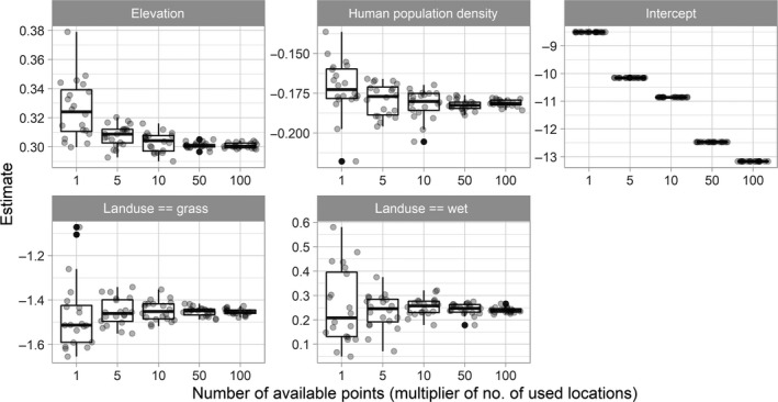
Estimated parameters in fitted habitat‐selection functions using increasing numbers of available points. Each dot represents an estimate from fitting a logistic regression model to 3004 GPS telemetry locations combined with a random sample of available points, with sample size given by the x‐axis (where 1 means 3,004 available points and 100 means 300,400 available points)
Let us consider the interpretation of the continuous covariates reflecting elevation and population density (Table 1, Model 1). Qualitatively, we might infer from the positive coefficient for elevation and negative coefficient for popden that, all other things being equal, Lupe is likely to select locations at higher elevations and in areas of lower population density. But, how do we interpret these coefficients quantitatively? Consider the following two locations, both in the same landcover class and with the same associated population density, but differing by 1 unit in elevation (since we have scaled this variable, a difference of 1 implies that the two observations differ by 1 SD in the original units of elevation):
location : elevation = 3, popden = 1.5, landuseC = wet
location : elevation = 2, popden = 1.5, landuseC = wet
TABLE 1.
Regression coefficients (SE) in fitted habitat‐selection functions fit to data from Lupe the fisher. Models 1 and 3 use forest as the reference level, Model 2 uses wet as the reference level. Model 3 includes interactions between elevation and landcover classes
| Model 1 | Model 2 | Model 3 | |
|---|---|---|---|
| (Intercept) | −13.168 | −12.918 | −13.171 |
| (0.019) | (0.107) | (0.020) | |
| elevation | 0.303 | 0.303 | 0.313 |
| (0.017) | (0.017) | (0.017) | |
| popden | −0.183 | −0.183 | −0.186 |
| (0.021) | (0.021) | (0.021) | |
| landuseCgrass | −1.477 | −1.471 | |
| (0.278) | (0.278) | ||
| landuseCwet | 0.250 | 0.183 | |
| (0.108) | (0.116) | ||
| landuseC1forest | −0.250 | ||
| (0.108) | |||
| landuseC1grass | −1.727 | ||
| (0.297) | |||
| elevation:landuseCgrass | 0.112 | ||
| (0.380) | |||
| elevation:landuseCwet | −0.498 | ||
| (0.127) |
Using Equation (6), we can calculate Lupe's relative use of location 1 versus location 2:
| (7) |
where we have dropped the integral from Equation (6) because it appears in both the numerator and denominator (and thus, cancels out). Now, if both locations are equally available, then , and we have:
| (8) |
Thus, we see that this ratio also provides an estimate of the relative intensity of use of the two locations (i.e. ), assuming the locations are equally available. In the context of habitat‐selection analyses, Avgar et al. (2017) refer to as quantifying relative selection strength (RSS).
Note that we would arrive at the exact same expression if we chose any two locations that differed by 1 unit of elevation and had the same values for popden and landuseC. Thus, quantifies the relative intensity of use of two locations that differ by 1 SD unit of elevation but are otherwise equivalent (i.e. they are equally available and have the same values of all other habitat covariates). If Lupe were to be presented with two such hypothetical locations, the model suggests she would be 1.35 times more likely to choose the one with the higher elevation. A similar interpretation can be ascribed to popden. Given two observations that differ by 1 SD unit of popden but are otherwise equal, Lupe would be times as likely to choose the location with higher population density (or, equivalently, times more likely to choose the location with the lower population density).
What about the coefficients for the landcover categories? Looking again at the regression output (Table 1, Model 1), we see that grass has a negative coefficient and wet has a positive coefficient. It is tempting to infer that Lupe spends most of her time in wet areas and rarely spends time in grassy habitats. As Figure 1 makes it clear, however, these inferences are not exactly correct. First, it is important to understand how categorical predictors are encoded in regression models. There are a number of different ways to parameterize the effect of categorical variables and unfamiliar readers may want to work through an introductory regression text (e.g. Chapter 6 of Kéry, 2010). The default coding in R is to treat one of the levels (whichever comes first alphanumerically) as a reference level and then to create a set of dummy variables that contrast the remaining levels of the categorical variable with this reference level. In our case, forest is the reference level. The coefficients associated with grass and wet represent contrasts between these land cover classes and the forest class. Qualitatively, we can use the signs and absolute magnitude of the coefficients for grass and wet to rank the landcover classes in terms of their relative selection strength, with grass < forest < wet. But again, how should we interpret the coefficients for grass and wet quantitatively?
Let us again consider two locations, this time assuming they have the same elevation and population densities, but with one location in wet and the other location in forest:
location : elevation = 2, popden = 1.5, landuseC = wet.
location : elevation = 2, popden = 1.5, landuseC = forest.
Lupe's relative use of location 1 relative to location 2 is given by (Equation 6):
| (9) |
Thus, assuming the two locations are equally available, we might infer that Lupe would be times more likely to choose the wet location than the location in forest. Of course, we know from Figure 1 that forest and wet are not equally available on the landscape. The higher availability of forest habitat implies that Lupe is more likely to be in forest than wet. We could attempt to correct for differences in availability within the MCP surrounding Lupe's locations by multiplying our result by the ratio of habitat availability for wet relative to forest habitats (2.3% vs. 95.7%; Figure 1). This gives us an adjusted ratio equal to exp(0.250)(0.023)/(0.957) = 0.03, suggesting we are times more likely to find Lupe in forest than wet habitat. With this calculation, we had to assume, perhaps naively, that the availability distributions for popden and elevation were the same in both wet and forest cover classes. In reality, if Lupe decides to move from forest to wet, it is likely that she will experience a change in elevation and popden too (i.e. these factors will not be held constant). To quantify Lupe's relative use of forest versus wet habitat, while also accounting for the effects other environmental characteristics that are associated with these habitat types, we can use integrated intensities—that is, we can integrate the spatial utilization distribution, , over all forest and wet habitats:
| (10) |
where and are indicator functions equal to 1 when location is in forest or wet respectively (and 0 otherwise). We can estimate this ratio using estimated HSF values, , at our set of available points drawn from within . Specifically, we sum the HSF values at all available points that fall in forest and them divide by the sum of HSF values for all available points falling in wet:
| (11) |
This ratio is also equal to 33, which agrees with the observed data; Lupe was found in forest habitat 33 times more often than in wet habitat (see Supporting Information Appendix A for code demonstrating how to calculate these quantities in R). Thus, we conclude Lupe is 33 times more likely to be found in forest than wet habitat (despite preferring wet over forest), assuming she restricts her movements to the MCP surrounding her observed locations and all of this MCP is equally available to her.
Before moving on, it is important to note that naively adjusted ratios (multiplying by availability of wet and forest habitats) and integrated intensities will not always agree. In fact, we find that they differ when comparing Lupe's relative use of wet versus grass habitat, with the integrated intensity better agreeing with the observed data (see Supporting Information Appendix A). Somewhat related, Avgar et al. (2017) suggested calculating average effects for continuous predictors, , by comparing the change in relative intensities from increasing by 1 unit (to ) to the average value of for all locations with . These average effects will also be influenced by cross‐correlations among predictor variables included in the model.
Instead of integrating over discrete cover types, we could integrate over specific geographical areas. For example, we could use integrated intensities to compare two areas in space, replacing the ‘landcover class’ indicator variables, and in Equation (11), with indicator variables for whether available locations fall in particular spatial regions. In addition, we could choose to change the area of interest (and thus, area of integration) from to , and then use the fitted model and Equation (6) to project how Lupe would spend her time in a novel environment (referred to as an ‘out‐of‐sample’ prediction). Despite the common reliance on HSFs as predictive models, out‐of‐sample predictions often suffer from poor accuracy, especially when compared to ‘in sample’ predictions, that is, predictions for the same area and time frame from which the original data were collected (Torres et al., 2015; Yates et al., 2018). We return to this important point in the discussion section.
Let's next consider what happens if we change the reference level of the land cover variable from forest to wet (Table 1, Model 2).
Lupe.dat <‐ within(Lupe.dat,


 landuseC1 <‐ relevel(landuseC, ref = "wet"))


 HSF.Lupe2 <‐ glm(case_ ~ elevation + popden + landuseC1,


 data = Lupe.dat,


 weight = w,


 family = binomial)
The coefficients for elevation and popden do not change. Note, however, that the coefficient for forest is negative despite Lupe using forest more than its availability (i.e. ) and Lupe spending more than 95% of her time in the forest! What is going on? Remember, the coefficients for categorical predictors reflect use:availability ratios for each level of the predictor relative to the use:availability ratio for the reference class. The coefficient for forest is negative because the use:availability ratio for forest is less than the use:availability ratio for the reference class, wet (see Figure 1). Depending on the reference level, it is possible to have a positive (negative) coefficient even when that landcover class is used more (less) than its availability. Furthermore, it is possible for a landcover class to be used frequently but have a negative coefficient. We have seen many ecologists, including some that are very quantitatively skilled and familiar with habitat‐selection models, make mistakes when interpreting coefficients associated with categorical predictors. This example also highlights the importance of plotting one's data (e.g. Figure 1) and considering habitat availability when interpreting regression coefficients. Plotting distributions of covariates for both used and available locations is one of the best ways to understand fitted habitat‐selection models, and is a good strategy to use for both continuous and categorical predictors (Fieberg, Forester, et al., 2018; Merow et al., 2013).
2.5. Interactions between environmental predictors
Consider the distribution of elevation at used and available locations across the different habitat classes (Figure 3). We see that there is a wider range of elevation in forest and wet habitat compared to grass habitat, and there is a clear association between elevation and landuseC, with higher median elevation at used locations in forest and grass habitat relative to wet habitat. Perhaps more importantly, we also see that values of elevation are higher, on average, for used locations (compared to available locations) in forest and grass, whereas the opposite is true in wet habitat. Although we should be skeptical of interactions that we discover while exploring our data (i.e. interactions that were not specified a priori), an analyst may be tempted to include an interaction between elevation and landuseC. In Model 3 (Table 1), we revert to having forest as the reference level and include the interaction between elevation and landuseC.
FIGURE 3.
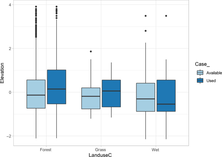
Distribution of elevation at used and available locations within each of three landcover types
Lupe.dat <‐ within(Lupe.dat, landuseC <‐ relevel(landuseC, ref = "forest"))


HSF.Lupe3 <‐ glm(case_ ~ elevation + popden + landuseC + elevation:landuseC,


 data = Lupe.dat,


 weight = w,


 family = binomial)
Using this syntax, R creates two new variables elevation:landuseCgrass equal to elevation when landuseC is grass and is 0 otherwise, and elevation:landuseCwet equal to elevation when landuseC is wet and is 0 otherwise. The coefficients associated with these predictors quantify the change in slope (i.e. change in the effect of elevation) when the locations fall in grass or wet, relative to the slope when the locations fall in forest. Starting from Equation (6) and using the estimates for Model 3 in Table 1, we can easily derive that the relative intensity of use of two equally available locations that differ by 1 SD unit of elevation is equal to when the two locations are in forest, when the locations are in grass, and when the locations are in wet habitat. Thus, we might conclude that Lupe would select for higher elevations when in forest or grass, but avoid higher elevations when in wet. Alternatively, we can consider how elevation changes Lupe's view of the different landcover categories, noting that elevation and elevation. Thus, we see that Lupe's relative avoidance of grass (relative to forest) and selection for wet (relative to forest) both decline with elevation, and Lupe's inherent ranking of these three habitat types will change as elevation increases. Both interpretations are statistically correct; the analyst chooses which one to use based on the ecological motivations for the analysis (the narrative sensu Otto & Rosales, 2020).
2.6. Nonlinear effects and other considerations
When building models, it is important to consider the functional relationships between different environmental characteristics and habitat use. For example, we may classify available predictors based on whether they represent resources (higher values are generally preferable), risks (lower values are generally preferable) or conditions (values that are not too high or too low are preferable; e.g. Matthiopoulos et al., 2020, 2015; Matthiopoulos, Fieberg, & Aarts, 2020). It is often useful to allow for nonlinear effects of conditions by including quadratic terms or using a set of spline basis functions. In either case, we end up requiring multiple coefficients to capture how the intensity of use changes with the environmental predictor. Consider, for example, that we could include a quadratic term to model the effect of elevation, with the expectation of a unimodal habitat‐selection function with respect to elevation. Estimating the relative use of locations and that differ in their values of elevation but are otherwise equivalent would be straightforward using Equation (6)—we would just need to calculate the ratio of relative intensities using coefficients for elevation and elevation2:
| (12) |
Avgar et al. (2017) provide simple formulas for calculating relative intensities under a number of different scenarios (e.g. models with quadratic polynomials, log‐transformed covariates and models with interactions). The log_rss function in the amt package (Signer et al., 2019) relies on R's generic predict function to aid the user in calculating the log relative intensity for any combination of model structure and two alternative locations; its use is illustrated in Supporting Information Appendix B. Understanding how these formulas are derived, however, helps build intuition and frees the user to construct estimators and estimation targets that capture relevant quantities of specific interest.
2.7. Statistical independence
An important assumption of the IPP model, and hence, habitat‐selection functions fitted to use‐availability data via logistic regression, is that any clustering of spatial locations can be explained solely by spatial covariates. Strictly speaking, this assumption will almost never be met, particularly with modern‐day telemetry studies that allow several locations to be collected on the same day. Telemetry observations close in time tend to also be close in space—that is, telemetry observations exhibit serial dependence (Fleming et al., 2014). This serial dependence is likely to manifest itself in residual spatial autocorrelation that could be modelled using a spatial random effect or a spatial predictor constructed to account for the effects of movement constraints on habitat availability (Johnson et al., 2013). Models with spatial random effects are, however, more complicated and difficult to fit.
Alternatively, if telemetry observations are collected at regular time intervals, then the locations may be argued to provide a representative sample of habitat use from a specific observation window (Fieberg, 2007; Otis & White, 1999). In these cases, it may be helpful to view our estimates of the parameters in our habitat‐selection function, , as useful summaries of habitat use for tagged individuals during these fixed time periods. Nevertheless, the assumption of independence of our locations is clearly problematic and will lead to estimates of uncertainty that are on average too small. If we are primarily interested in population‐level inferences, then we may choose to ignore within‐individual autocorrelation when estimating individual‐specific coefficients but use a robust form of SE that treats individuals as independent when describing uncertainty in population‐level parameters (e.g. using a bootstrap; Fieberg et al., 2020) or generalized estimating equations approach (e.g. Fieberg et al., 2009, 2010; Koper & Manseau, 2009).
3. STEP‐SELECTION FUNCTIONS
Step‐selection functions were developed to deal with serial dependence as well as temporally varying availability distributions resulting from movement constraints (Fortin et al., 2005; Thurfjell et al., 2014). Rather than treat locations as independent and identically distributed (with availability that does not depend on time), step‐selection functions model transitions, or ‘steps’, connecting sequential locations ( units apart) in geographical space. The resulting redistribution kernel takes the general form:
| (13) |
where gives the conditional probability of finding the individual at location at time given it was at location at time , is referred to as a step‐selection function, and is a selection‐free movement kernel that describes how the animal would move in homogeneous habitat or in the absence of habitat selection (i.e. when = a constant for all ). Note that we represent the parameter vectors ( and ) as functions of the step duration . This notation reflects the fact that step‐selection parameters are scale dependent (i.e. different 's will result in different estimates of and ; see Avgar et al., 2016 for more details). Thus, we generally require observations to be equally spaced in time (but see Munden et al., 2020), and care must be taken when comparing inference from models fitted at different temporal resolution. When animals are observed at irregular time intervals, as with many marine species, it is possible to first fit a continuous‐time movement model to the location data and then use this model to provide multiply imputed datasets that are regularly spaced in time (see e.g. McClintock, 2017).
As with habitat‐selection functions, it is typical to model as a loglinear function of spatial covariates and regression parameters, . A key difference between habitat‐selection functions and step‐selection functions, however, is that the latter allow the available distribution to be time dependent and equal to . Consequently, step‐selection functions allow explicit consideration of temporally dynamic environmental covariates, and (and, possibly, environmental covariates measured along the path between these two locations). One option that often performs well and enhances interpretability is to include habitat covariates at the start of the movement step in the model for , and habitat covariates at the end of the movement step in the model for ; we provide an example in Supporting Information Appendix B. This approach allows us to separately model the effect of habitat on accessibility (through the model for ) and selection (through the model for ; Matthiopoulos, 2003), and results in a more general formulation: . We recognize, however, that there may be covariates, often measured along a movement path (e.g. crossing of a road or passing over an extremely steep slope), that also influence accessibility but that may be best included in the model for . In general, we recommend including covariates in the model for when they are likely to influence general movement characteristics and in the model for when they are likely to influence the overall attractiveness of a more limited region of geographical space.
3.1. Models for ϕ(s, s′; γ(Δt))
Step‐selection functions build on an early idea by Arthur et al. (1996) to model time‐dependent availability via a circular buffer with radius centred on the previous location. Rhodes et al. (2015) showed that this model is equivalent to assuming:
| (14) |
where is the Euclidean distance between locations and , referred to as the step length. Rhodes et al. (2015) also demonstrated that circular buffers imply that individuals are more likely to move large distances than short distances since there is more area, and thus probability, associated with outer rings of the circle. Instead, they suggested using an exponential distribution to accommodate right‐skewed step‐length distributions and a tendency for animals to make shorter rather than longer movements:
| (15) |
Rather than specify a model directly in terms of , it is more common to see movement kernels specified in terms of the distribution of step lengths, , and turn angles (changes in direction from the previous bearing), . In the sections that follow, we will let and represent step‐length and turn‐angle distributions respectively. Step‐selection analyses frequently use either an exponential or gamma distribution for . Turn angles may be assumed to be uniformly distributed as in Arthur et al. (1996) and Rhodes et al. (2015). Alternatively, circular distributions, such as the von Mises distribution or wrapped Cauchy or Weibull distributions, allow for a mode at 0 and can thus accommodate correlated movements (i.e. sequential steps are assumed, on average, to follow in the same direction as the previous step).
Although step‐length and turn‐angle distributions are typically assumed to be independent, animals commonly exhibit a mix of temporally persistent movement behaviours, ranging between high‐displacement movements (e.g. when travelling between habitat patches, migrating, or dispersing) and low‐displacement movements (e.g. during foraging or resting bouts). If positional data are collected more frequently than the occurrence of behavioural switches, we might expect a negative cross‐correlation between step lengths and turn angles (moving far is likely to coincide with moving straight) and a positive autocorrelation between the current and previous step lengths and turn angles. Moreover, as implied by the more flexible formulation, , both step‐length and turn‐angle distribution may shift as a function of spatial and/or temporal covariates such as habitat permeability (e.g. terrain ruggedness, snow depth or vegetation density), time of day, season and predation risk (Avgar et al., 2013, 2016). Thus, although is a ‘selection‐free’ movement kernel, it may still depend on environmental or temporal covariates, and hence, may vary through space and time, resulting in both auto‐ and cross‐correlations in step attributes.
Cross‐correlation between step lengths and turn angles is difficult to model with common statistical distributions, but could be accommodated using copulae (Durante & Sempi, 2010). Alternatively, one could resample (i.e. bootstrap) step length and turn angle pairs, , to preserve any correlation that is present in the data (Fortin et al., 2005). Although we generally find the bootstrap appealing (Fieberg et al., 2020), it has limitations in this context. In particular, the observed distribution of step lengths and turn angles will reflect both inherent movement characteristics of the species (captured by ) as well as habitat selection (captured by ). Using the observed steps as a nonparametric model for without adjustment for the effect of can result in biased estimates of (Forester, Im, & Rathouz, 2009). We will return to this point in the next section. As mentioned previously (see Section 3), and regardless of the source of correlation, it may be preferable to calculate robust SEs by treating individuals as the relevant sampling unit when performing population‐level inference (e.g. Prima et al., 2017). Lastly, cross‐ and autocorrelations in step lengths and turn angles, as well as their dependencies on various temporal or environmental characteristics, could be modelled parametrically using an integrated step‐selection function (Avgar et al., 2016). To do so, we need to include appropriate statistical interactions (e.g. between concurrent and previous step lengths/turn angles and between these step attributes and environmental or temporal covariates). We discuss this process further below, and provide examples in the Supporting Information Appendix B. See also Prokopenko et al. (2017), Scrafford et al. (2018) and Dickie et al. (2020).
3.2. Estimation of movement and habitat‐selection parameters
Although it is possible to simultaneously estimate movement () and habitat‐selection () parameters using maximum likelihood (e.g. Rhodes et al., 2015) or Bayesian methods (e.g. Johnson et al., 2008), this is rarely done in practice as it would require custom‐written code. Instead, it is common to use the following approach:
Estimate or approximate using observed step lengths and turn angles, giving .
Generate time‐dependent available locations by simulating potential movements from the previously observed location, . Similar to applications of HSFs, it is up to the user to decide how many available locations to sample for each used location, and, due to similar considerations (properly approximating the availability domain: , the more points the merrier).
Estimate using conditional logistic regression, with strata formed by combining time‐dependent used and available locations.
If we knew and could simulate directly from it (skipping step 1), then this approach would provide unbiased estimates of (Forester et al., 2009). However, as mentioned in the previous section, estimating the selection‐free movement kernel, , from observed steps without adjusting for habitat selection, via , can lead to biased estimates of and .
Forester et al. (2009) considered the case where the step‐length distribution, , is given by an exponential distribution with unknown parameter, . They showed that estimating directly from the observed distribution of step lengths (without adjusting for the effect of , and then proceeding with steps 2 and 3 results in a biased estimators of . Forester et al. (2009) also showed that the bias (if is given by an exponential distribution) is eliminated if is included as a predictor in the model. Avgar et al. (2016) further showed that the coefficient associated with could be used to modify , leading to an unbiased estimator of and thus, . In addition, they showed how similar adjustments could be used to obtain unbiased estimators of step‐length () and habitat‐selection () parameters when the distribution of step lengths is given by a gamma, half‐normal or log‐normal distribution. Similarly, Duchesne et al. (2015) showed that including as a predictor can lead to unbiased estimators of turn angle parameters () when the distribution of turn angles follows a von Mises distribution. All of these adjustments are available in the amtpackage (Signer et al., 2019). Avgar et al. (2016) coined the term integrated step‐selection analysis to emphasize that these results provide new opportunities to model both movement and habitat selection via tried and true statistical software for fitting conditional logistic regression models.
In Supporting Information Appendix B, we provide a ‘How to’ guide for implementing an integrated step‐selection analysis using the amt package in R (R Core Team, 2019; Signer et al., 2019). Conducting an integrated step‐selection analysis requires, in addition to the three steps outlined in this section, that we add a fourth step that re‐estimates the movement parameters in using regression coefficients associated with movement characteristics (e.g. , ). This last step adjusts the parameters in to account for the effect of habitat selection when estimating the movement kernel (Avgar et al., 2016), and is hence unnecessary if no inference about movement is being made. The details of how to carry on these adjustments are provided in Supporting Information Appendix C and in Avgar et al. (2016). Importantly, interactions may be included between movement characteristics (e.g. , ) and environmental covariates, , to allow the movement kernel to depend on the environment. When interactions are included, step 4 results in a movement kernel, , that depends on the habitat the animal is in at the start of the movement step (Figure 4).
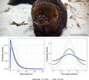
FIGURE 4.
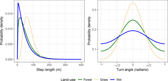
Step‐length and turn‐angle distributions from an integrated step‐selection analysis applied to Lupe's location data (see Supporting Information Appendix B). The conditional logistic regression model included interactions between movement characteristics (step length, log step length and cosine of the turn angle) and the landuse category Lupe was in at the start of the movement step. We see that Lupe tends to take larger, more directed steps when in grass and slower and more tortuous steps in wet habitat
3.3. Interpretation of parameters in an integrated step‐selection analysis
The habitat‐selection parameters in an SSF can be interpreted in the same way as habitat‐selection parameters in HSFs (i.e. as relative intensities, assuming locations are equally available and differing in terms of a single habitat covariate). Hence, the expressions in Avgar et al. (2017), and the log_rss function in amt, are suitable for calculating and interpreting the effects of the various habitat covariates. However, it is important to recognize that the used and available distributions in step‐selection analyses are dynamic and non‐uniform in space. In particular, they depend on an individual's current location and movement tendencies (as well as the observed time‐scale determined by ; Barnett & Moorcroft, 2008; Signer et al., 2017). Thus, questions that require integrating intensities over space (e.g. Equation 10) are more difficult to address. Possible solutions include using simulation modelling (Signer et al., 2017), solving the master equation (formed by multiplying the right‐hand side of Equation (13) by and then integrating over with respect to ) for its steady state (Potts, Bastille‐Rousseau, et al., 2014; Potts, Mokross, et al., 2014), or in some cases, translating the fitted model into a partial differential equation model with analytical steady‐state distribution (Potts & Schlägel, 2020). We also note that alternative modelling frameworks exist with parameters that directly describe relative intensities of use at both fine and coarse scales (e.g. Michelot, Blackwell, et al., 2019, 2020; Michelot, Gloaguen, et al., 2019). These new analytical developments hold exciting promises to bridge the micro scale of animal movement behaviour with the macro scale of animal spatial distribution but are more computationally challenging to implement. Most importantly, biologists need to be aware that parameters that describe habitat selection at local and macro scales may differ, and thus, extra steps may be required to translate movement dynamics captured by integrated step‐selection analyses to the coarser scales typically modelled with traditional habitat‐selection functions. The amt package has a basic capacity to simulate the utilization distribution based on a parameterized integrated step‐selection function (Signer et al., 2017), and we expect this approach to become more flexible in the near future, allowing users to forecast not only steady‐state utilization distributions but also transient movement patterns such as migration and dispersal.
Using an integrated step‐selection approach (e.g. as in Figure 4), it is also possible to draw ecological inference using the selection‐free movement kernel. For example, the fitted step‐length and turn‐angle distributions can tell us how much more likely an animal is to take large versus small steps or to turn left or right relative to moving straight. We can also calculate moments of these distributions under different environmental conditions, which can be informative when our models include interactions between movement characteristics and environmental predictors. For example, we could calculate the expected selection‐free displacement rates (and/or directionality) as function of local snow depth (i.e. if snow depth was included in our model as an interaction with step length). Once the selection‐free movement parameters are obtained, one can use them to calculate various aspects of the (theoretical) distributions of step lengths and turn angles, such as the mean, the median or the 95% confidence bounds (see Supporting Information Appendix B for examples).
4. DISCUSSION
We have highlighted how connecting habitat‐selection functions to IPP models and weighted distribution theory helps with interpreting parameters in habitat‐selection functions using simple examples. We have also reviewed step‐selection functions and demonstrated how to estimate movement and habitat‐selection parameters when conducting an integrated step‐selection analysis using the amt package. So far, we have focused on interpreting results when analysing data from a single individual. We end with a brief discussion addressing statistical dependencies, particularly when analysing data from multiple individuals, along with issues related to model transferability and parameter sensitivity to changes in habitat availability and species population density.
4.1. Statistical dependencies
Earlier, we highlighted the importance of statistical independence as it applies to individual locations when estimating habitat‐selection functions. We also noted that step‐selection analyses typically assume step lengths and turn angles are independent of each other and also over time, although it is possible to account for these correlations using appropriate interactions (e.g. between step length at time and time , step length and turn angle both at time ). It would be nice to have multivariate distributions available that are capable of describing correlated step lengths and turn angles and any inherent autocorrelation. It is plausible, however, that models that allow movement parameters to vary by habitat type, using interactions between step length, turn angle and habitat covariates, will be able to account for much of the autocorrelation and cross‐correlation (between step lengths and turn angles) present in the data. Similarly, autocorrelation and cross‐correlations may be accommodated by models that include a (possibly latent) behavioural state, with movement and habitat‐selection parameters that are state dependent (Nicosia et al., 2017; Suraci et al., 2019).
In addition to cross‐correlation between step lengths and turn angles and serial dependencies, individuals living in different environments may exhibit different habitat‐selection patterns, and thus, repeated observations on the same set of individuals will induce further statistical dependencies. A simple strategy for dealing with repeated measures when individuals can be assumed to be independent is to fit models to individual animals and then treat the resulting coefficients as data when inferring population‐level patterns (Fieberg et al., 2010; Murtaugh, 2007). For example, sample means of the regression coefficients can be used to characterize average habitat‐selection parameters. Estimating among‐animal variability is trickier due to sampling error; naively ignoring sampling error will lead to a positive bias in estimates of among‐animal variability, but more formal two‐step methods can address this issue (Craiu et al., 2011, 2016; Dickie et al., 2020). Alternatively, generalized linear mixed models with random coefficients can be used to quantify among‐animal variability in habitat‐selection analyses (Muff et al., 2020).
Although it is possible to conduct integrated step‐selection analyses with hierarchical models containing random effects, we have much to learn about how these approaches perform in practice. For example, Muff et al. (2020) found that parameters describing among‐animal variability in habitat‐selection parameters were biased low when movement characteristics were included in the model. Mixed‐effect models with random coefficients are also ‘parameter hungry’, requiring variance and covariance parameters to be estimated, where is the number of random coefficients. Models that allow all coefficients to be animal specific and to covary are thus likely to be computationally challenging to fit and problematic for small datasets containing only a few individuals. For this reason, Muff et al. (2020) assumed coefficients did not covary in their applied examples. In the context of our fisher analysis, this equates to assuming that knowing an individual's coefficient for popden tells us nothing about that animal's parameters for elevation or landuseC variables. For categorical variables, it is natural to expect parameters to have a negative covariance (since, e.g. spending more time in forest must come at the expense of spending less time in other landuse categories). Research evaluating the performance of mixed‐effect step‐selection analyses under various data‐generating scenarios would be helpful for evaluating robustness to assumption violations (e.g. those regarding the distribution of random parameters).
4.2. Sensitivity of selection coefficients to species population density and habitat availability
Before concluding, we feel it is important to briefly discuss the oft observed pattern of density and availability dependence in habitat‐selection inference (Matthiopoulos et al., 2011, 2015; Matthiopoulos, Fieberg, & Aarts, 2020; Mysterud & Ims, 1998). Density‐dependent inference may be observed when the same analysis is applied to individuals or populations of the same species, under similar environmental conditions, but at different population densities. Availability dependence (also referred to as a ‘functional response’) may be observed when the same analysis is applied to individuals or populations of the same species, which experience different landscape‐scale resource or habitat availabilities. For example, van Beest et al. (2016) found that individual elk display availability‐dependent habitat‐selection patterns (switching from selection to avoidance of certain habitats as function of the availability of these habitats within their home range), but that the strength of this functional response depended on elk population density. Such context dependencies are in fact so common that we do not know of a single instance where researchers were looking for them and failed to find them. Recently, Avgar et al. (2020) showed that such context dependencies in habitat‐selection patterns are expected to emerge even under the simplest theoretical model of an Ideal Free Distribution (Fretwell, 1969). Thus, habitat‐selection models often have poor predictive capacity when transferred across different study areas, or even within the same area over time (e.g. Torres et al., 2015). Yet, these differences may also be exploited; modelling frameworks that leverage data from multiple environments and across a range of population densities can potentially increase predictive capabilities (Matthiopoulos et al., 2019). As with any other attempt to model complex ecological data, critical evaluation of model performance for both within and out‐of‐sample data is essential (Fieberg, Forester, et al., 2018).
AUTHORS' CONTRIBUTIONS
J.F. developed the idea for the review, led the writing of the manuscript and drafted the initial version of Supporting Information Appendix A; B.S. and J.S. drafted the initial version of Supporting Information Appendix B; B.S. and T.A. drafted the initial version of Supporting Information Appendix C. All authors contributed critically to the manuscript text and Supporting Information, and gave final approval for publication.
Supporting information
Appendix
ACKNOWLEDGEMENTS
We thank J.R. Potts, three anonymous reviewers and the Associate Editor for helpful comments that improved the manuscript. J.F. received partial salary support from the Minnesota Agricultural Experimental Station. T.A. received partial salary support from the Utah Agricultural Experimental Station.
Fieberg J, Signer J, Smith B, Avgar T. A ‘How to’ guide for interpreting parameters in habitat‐selection analyses. J Anim Ecol. 2021;90:1027–1043. 10.1111/1365-2656.13441
[The copyright line for this article was changed on 24 March 2021 after original online publication.]
Handling Editor Anne Loison
DATA AVAILABILITY STATEMENT
All of the data used in this paper are available from within the amt package (Signer et al., 2019). We have also archived the data and our code in the Data Repository of the University of Minnesota (Fieberg et al., 2021).
REFERENCES
- Aarts, G. , Fieberg, J. , & Matthiopoulos, J. (2012). Comparative interpretation of count, presence–absence and point methods for species distribution models. Methods in Ecology and Evolution, 3(1), 177–187. 10.1111/j.2041-210X.2011.00141.x [DOI] [Google Scholar]
- Aarts, G. , MacKenzie, M. , McConnell, B. , Fedak, M. , & Matthiopoulos, J. (2008). Estimating space‐use and habitat preference from wildlife telemetry data. Ecography, 31(1), 140–160. 10.1111/j.2007.0906-7590.05236.x [DOI] [Google Scholar]
- Arthur, S. M. , Manly, B. F. , McDonald, L. L. , & Garner, G. W. (1996). Assessing habitat selection when availability changes. Ecology, 77(1), 215–227. 10.2307/2265671 [DOI] [Google Scholar]
- Avgar, T. , Betini, G. S. , & Fryxell, J. M. (2020). Habitat selection patterns are density‐dependent under the Ideal Free Distribution. Journal of Animal Ecology, 89(12), 2777–2787. 10.1111/1365-2656.13352 [DOI] [PMC free article] [PubMed] [Google Scholar]
- Avgar, T. , Lele, S. R. , Keim, J. L. , & Boyce, M. S. (2017). Relative selection strength: Quantifying effect size in habitat‐and step‐selection inference. Ecology and Evolution, 7(14), 5322–5330. 10.1002/ece3.3122 [DOI] [PMC free article] [PubMed] [Google Scholar]
- Avgar, T. , Mosser, A. , Brown, G. S. , & Fryxell, J. M. (2013). Environmental and individual drivers of animal movement patterns across a wide geographical gradient. Journal of Animal Ecology, 82(1), 96–106. 10.1111/j.1365-2656.2012.02035.x [DOI] [PubMed] [Google Scholar]
- Avgar, T. , Potts, J. R. , Lewis, M. A. , & Boyce, M. S. (2016). Integrated step selection analysis: Bridging the gap between resource selection and animal movement. Methods in Ecology and Evolution, 7(5), 619–630. 10.1111/2041-210X.12528 [DOI] [Google Scholar]
- Barnett, A. H. , & Moorcroft, P. R. (2008). Analytic steady‐state space use patterns and rapid computations in mechanistic home range analysis. Journal of Mathematical Biology, 57(1), 139–159. 10.1007/s00285-007-0149-8 [DOI] [PubMed] [Google Scholar]
- Boyce, M. S. , & McDonald, L. L. (1999). Relating populations to habitats using resource selection functions. Trends in Ecology & Evolution, 14(7), 268–272. 10.1016/S0169-5347(99)01593-1 [DOI] [PubMed] [Google Scholar]
- Boyce, M. S. , Vernier, P. R. , Nielsen, S. E. , & Schmiegelow, F. K. A. (2002). Evaluating resource selection functions. Ecological Modelling, 157(2), 281–300. 10.1016/S0304-3800(02)00200-410.1016/S0304-3800(02)00200-4 [DOI] [Google Scholar]
- Center for International Earth Science Information Network (CIESIN) Columbia University, & CIAT, Centro Internacional de Agricultura Tropical . (2005, 20190227). Gridded population of the world, version 3 (gpwv3): Population density grid. NASA Socioeconomic Data; Applications Center (SEDAC). Retrieved from 10.7927/H4XK8CG2 [DOI] [Google Scholar]
- Chamaille‐Jammes, S. (2019). A reformulation of the selection ratio shed light on resource selection functions and leads to a unified framework for habitat selection studies. bioRxiv. 10.1101/56583810.1101/565838 [DOI] [Google Scholar]
- Craiu, R. V. , Duchesne, T. , Fortin, D. , & Baillargeon, S. (2011). Conditional logistic regression with longitudinal follow‐up and individual‐level random coefficients: A stable and efficient two‐step estimation method. Journal of Computational and Graphical Statistics, 20(3), 767–784. 10.1198/jcgs.2011.09189 [DOI] [Google Scholar]
- Craiu, R. , Duchesne, T. , Fortin, D. , & Baillargeon, S. (2016). TwoStepCLogit: Conditional logistic regression: A two‐step estimation method. R package version 1.2. 5. [Google Scholar]
- Cressie, N. (1992). Statistics for spatial data. Terra Nova, 4(5), 613–617. 10.1111/j.1365-3121.1992.tb00605.x [DOI] [Google Scholar]
- Defourny, P. , Schouten, L. , Bartalev, S. , Bontemps, S. , Cacetta, P. , De Wit, A. , di Bella, C. , Gérard, B. , Giri, C. , Gond, V. , Hazeu, G. W. , Heinimann, A. , Herold, M. , Jaffrain, G. , Latifovic, R., Lin, H. , Mayaux, P. , Mücher, C. A. , Nonguiera, A. , … Arino, O. (2009). Accuracy assessment of a 300 m global land cover map. The GlobCover Experience. [Google Scholar]
- Dickie, M. , McNay, S. R. , Sutherland, G. D. , Cody, M. , & Avgar, T. (2020). Corridors or risk? Movement along, and use of, linear features varies predictably among large mammal predator and prey species. Journal of Animal Ecology, 89(2), 623–634. 10.1111/1365-2656.13130 [DOI] [PMC free article] [PubMed] [Google Scholar]
- Dodge, S. , Bohrer, G. , Weinzierl, R. , Davidson, S. C. , Kays, R. , Douglas, D. , & Wikelski, M. (2013). The environmental‐data automated track annotation (env‐data) system: Linking animal tracks with environmental data. Movement Ecology, 1(1), 3. 10.1186/2051-3933-1-3 [DOI] [PMC free article] [PubMed] [Google Scholar]
- Duchesne, T. , Fortin, D. , & Rivest, L.‐P. (2015). Equivalence between step selection functions and biased correlated random walks for statistical inference on animal movement. PLoS One, 10(4), e0122947. 10.1371/journal.pone.0122947 [DOI] [PMC free article] [PubMed] [Google Scholar]
- Durante, F. , & Sempi, C. (2010). Copula theory: An introduction. In Jaworski P., Durante F., Härdle W. K., & Rychlik T. (Eds.), Copula theory and its applications (pp. 3–31). Springer. [Google Scholar]
- Elith, J. , & Leathwick, J. R. (2009). Species distribution models: Ecological explanation and prediction across space and time. Annual Review of Ecology, Evolution, and Systematics, 40(1), 677. 10.1146/annurev.ecolsys.110308.120159 [DOI] [Google Scholar]
- Elith, J. , Phillips, S. J. , Hastie, T. , Dudik, M. , Chee, Y. E. , & Yates, C. J. (2011). A statistical explanation of MaxEnt for ecologists. Diversity and Distributions, 17(1), 43–57. 10.1111/j.1472-4642.2010.00725.x [DOI] [Google Scholar]
- Fieberg, J. (2007). Kernel density estimators of home range: Smoothing and the autocorrelation red herring. Ecology, 88(4), 1059–1066. 10.1890/06-0930 [DOI] [PubMed] [Google Scholar]
- Fieberg, J. , Bohrer, G. , Davidson, S. , & Kays, R. (2018). Short course on analyzing animal tracking data. Presented at the North Carolina Museum of Natural Sciences. May 21–23, 2018. Retrieved from https://movebankworkshopraleighnc.netlify.com/index.html [Google Scholar]
- Fieberg, J. , Forester, J. D. , Street, G. M. , Johnson, D. H. , ArchMiller, A. A. , & Matthiopoulos, J. (2018). Used‐habitat calibration plots: A new procedure for validating species distribution, resource selection, and step‐selection models. Ecography, 41(5), 737–752. 10.1111/ecog.03123 [DOI] [Google Scholar]
- Fieberg, J. , Matthiopoulos, J. , Hebblewhite, M. , Boyce, M. S. , & Frair, J. L. (2010). Correlation and studies of habitat selection: Problem, red herring or opportunity? Philosophical Transactions of the Royal Society of London B: Biological Sciences, 365(1550), 2233–2244. 10.1098/rstb.2010.0079 [DOI] [PMC free article] [PubMed] [Google Scholar]
- Fieberg, J. , Rieger, R. H. , Zicus, M. C. , & Schildcrout, J. S. (2009). Regression modelling of correlated data in ecology: Subject‐specific and population averaged response patterns. Journal of Applied Ecology, 46(5), 1018–1025. 10.1111/j.1365-2664.2009.01692.x [DOI] [Google Scholar]
- Fieberg, J. , Signer, J. , Smith, B. , & Avgar, T. (2021). R code and output supporting: A ‘how‐to’ guide for interpreting parameters in habitat‐selection analyses. Data Repository for the University of Minnesota. https://hdl.handle.net/11299/218272 [DOI] [PMC free article] [PubMed] [Google Scholar]
- Fieberg, J. R. , Vitense, K. , & Johnson, D. H. (2020). Resampling‐based methods for biologists. PeerJ, 8, e9089. [DOI] [PMC free article] [PubMed] [Google Scholar]
- Fithian, W. , & Hastie, T. (2013). Finite‐sample equivalence in statistical models for presence‐only data. The Annals of Applied Statistics, 7(4), 1917. 10.1214/13-AOAS667 [DOI] [PMC free article] [PubMed] [Google Scholar]
- Fleming, C. H. , Calabrese, J. M. , Mueller, T. , Olson, K. A. , Leimgruber, P. , & Fagan, W. F. (2014). From fine‐scale foraging to home ranges: A semivariance approach to identifying movement modes across spatiotemporal scales. The American Naturalist, 183(5), E154–E167. [DOI] [PubMed] [Google Scholar]
- Forester, J. D. , Im, H. K. , & Rathouz, P. J. (2009). Accounting for animal movement in estimation of resource selection functions: Sampling and data analysis. Ecology, 90(12), 3554–3565. [DOI] [PubMed] [Google Scholar]
- Fortin, D. , Beyer, H. L. , Boyce, M. S. , Smith, D. W. , Duchesne, T. , & Mao, J. S. (2005). Wolves influence elk movements: Behavior shapes a trophic cascade in Yellowstone National Park. Ecology, 86(5), 1320–1330. [Google Scholar]
- Fretwell, S. D. (1969). On territorial behavior and other factors influencing habitat distribution in birds. Acta Biotheoretica, 19(1), 45–52. [Google Scholar]
- Guisan, A. , Thuiller, W. , & Zimmermann, N. E. (2017). Habitat suitability and distribution models: With applications in R. Cambridge University Press. [Google Scholar]
- Hirzel, A. H. , & Le Lay, G. (2008). Habitat suitability modelling and niche theory. Journal of Applied Ecology, 45(5), 1372–1381. [Google Scholar]
- Hooten, M. B. , Hanks, E. M. , Johnson, D. S. , & Alldredge, M. W. (2013). Reconciling resource utilization and resource selection functions. Journal of Animal Ecology, 82(6), 1146–1154. [DOI] [PubMed] [Google Scholar]
- Hooten, M. B. , Johnson, D. S. , McClintock, B. T. , & Morales, J. M. (2017). Animal movement: Statistical models for telemetry data. CRC Press. [Google Scholar]
- Hosmer, D. W. , Lemeshow, S. , & Sturdivant, R. X. (2013). Applied logistic regression (Vol. 398). John Wiley & Sons. [Google Scholar]
- Johnson, C. J. , Nielsen, S. E. , Merrill, E. H. , McDonald, T. L. , & Boyce, M. S. (2006). Resource selection functions based on use‐availability data: Theoretical motivation and evaluation methods. Journal of Wildlife Management, 70(2), 347–357. [Google Scholar]
- Johnson, D. H. (1980). The comparison of usage and availability measurements for evaluating resource preference. Ecology, 61(1), 65–71. 10.2307/1937156 [DOI] [Google Scholar]
- Johnson, D. S. , Hooten, M. B. , & Kuhn, C. E. (2013). Estimating animal resource selection from telemetry data using point process models. Journal of Animal Ecology, 82(6), 1155–1164. 10.1111/1365-2656.12087 [DOI] [PubMed] [Google Scholar]
- Johnson, D. S. , Thomas, D. L. , Ver Hoef, J. M. , & Christ, A. (2008). A general framework for the analysis of animal resource selection from telemetry data. Biometrics, 64(3), 968–976. 10.1111/j.1541-0420.2007.00943.x [DOI] [PubMed] [Google Scholar]
- Kays, R. , Crofoot, M. C. , Jetz, W. , & Wikelski, M. (2015). Terrestrial animal tracking as an eye on life and planet. Science, 348(6240), aaa2478. 10.1126/science.aaa2478 [DOI] [PubMed] [Google Scholar]
- Keating, K. A. , & Cherry, S. (2004). Use and interpretation of logistic regression in habitat‐selection studies. Journal of Wildlife Management, 68(4), 774–789. [Google Scholar]
- Kéry, M. (2010). Introduction to WinBUGS for ecologists: Bayesian approach to regression, ANOVA, mixed models and related analyses. Academic Press. [Google Scholar]
- Koper, N. , & Manseau, M. (2009). Generalized estimating equations and generalized linear mixed‐effects models for modelling resource selection. Journal of Applied Ecology, 46(3), 590–599. 10.1111/j.1365-2664.2009.01642.x [DOI] [Google Scholar]
- LaPoint, S. , Gallery, P. , Wikelski, M. , & Kays, R. (2013a). Animal behavior, cost‐based corridor models, and real corridors. Landscape Ecology, 28(8), 1615–1630. 10.1007/s10980-013-9910-0 [DOI] [Google Scholar]
- LaPoint, S. , Gallery, P. , Wikelski, M. , & Kays, R. (2013b). Data from: Animal behavior, cost‐based corridor models, and real corridors. Movebank Data Repository, 10.5441/001/1.2tp2j43g [DOI] [Google Scholar]
- Lele, S. R. , & Keim, J. L. (2006). Weighted distributions and estimation of resource selection probability functions. Ecology, 87(12), 3021–3028. [DOI] [PubMed] [Google Scholar]
- Lele, S. R. , Merrill, E. H. , Keim, J. , & Boyce, M. S. (2013). Selection, use, choice and occupancy: Clarifying concepts in resource selection studies. Journal of Animal Ecology, 82(6), 1183–1191. 10.1111/1365-2656.12141 [DOI] [PubMed] [Google Scholar]
- Manly, B. , McDonald, L. , Thomas, D. , McDonald, T. L. , & Erickson, W. P. (2002). Resource selection by animals: Statistical design and analysis for field studies. Springer Science & Business Media. [Google Scholar]
- Matthiopoulos, J. (2003). The use of space by animals as a function of accessibility and preference. Ecological Modelling, 159(2–3), 239–268. 10.1016/S0304-3800(02)00293-4 [DOI] [Google Scholar]
- Matthiopoulos, J. , Fieberg, J. , & Aarts, G. (2020). Species‐habitat associations: Spatial data, predictive models, and ecological insights. University of Minnesota Libraries Publishing: Retrieved from the University of Minnesota Digital Conservancy. http://hdl.handle.net/11299/217469 [Google Scholar]
- Matthiopoulos, J. , Fieberg, J. , Aarts, G. , Barraquand, F. , & Kendall, B. E. (2020). Within reach? Habitat availability as a function of individual mobility and spatial structuring. The American Naturalist, 195(6), 1009–1026. 10.1086/708519 [DOI] [PubMed] [Google Scholar]
- Matthiopoulos, J. , Fieberg, J. , Aarts, G. , Beyer, H. L. , Morales, J. M. , & Haydon, D. T. (2015). Establishing the link between habitat selection and animal population dynamics. Ecological Monographs, 85(3), 413–436. 10.1890/14-2244.1 [DOI] [Google Scholar]
- Matthiopoulos, J. , Field, C. , & MacLeod, R. (2019). Predicting population change from models based on habitat availability and utilization. Proceedings of the Royal Society B: Biological Sciences, 286(1901), 20182911. 10.1098/rspb.2018.2911 [DOI] [PMC free article] [PubMed] [Google Scholar]
- Matthiopoulos, J. , Hebblewhite, M. , Aarts, G. , & Fieberg, J. (2011). Generalized functional responses for species distributions. Ecology, 92(3), 583–589. 10.1890/10-0751.1 [DOI] [PubMed] [Google Scholar]
- McClintock, B. T. (2017). Incorporating telemetry error into hidden markov models of animal movement using multiple imputation. Journal of Agricultural, Biological and Environmental Statistics, 22(3), 249–269. 10.1007/s13253-017-0285-6 [DOI] [Google Scholar]
- Merow, C. , Smith, M. J. , & Silander, J. A. (2013). A practical guide to maxent for modeling species' distributions: What it does, and why inputs and settings matter. Ecography, 36(10), 1058–1069. 10.1111/j.1600-0587.2013.07872.x [DOI] [Google Scholar]
- Michelot, T. , Blackwell, P. G. , Chamaillé‐Jammes, S. , & Matthiopoulos, J. (2020). Inference in MCMC step selection models. Biometrics, 76(2), 438–447. 10.1111/biom.13170 [DOI] [PubMed] [Google Scholar]
- Michelot, T. , Blackwell, P. G. , & Matthiopoulos, J. (2019). Linking resource selection and step selection models for habitat preferences in animals. Ecology, 100(1). 10.1002/ecy.2452 [DOI] [PubMed] [Google Scholar]
- Michelot, T. , Gloaguen, P. , Blackwell, P. G. , & Étienne, M.‐P. (2019). The langevin diffusion as a continuous‐time model of animal movement and habitat selection. Methods in Ecology and Evolution, 10(11), 1894–1907. 10.1111/2041-210X.13275 [DOI] [Google Scholar]
- Millspaugh, J. J. , Nielson, R. M. , McDonald, L. , Marzluff, J. M. , Gitzeồn, R. A. , Rittenhouse, C. D. , & Sheriff, S. L. (2006). Analysis of resource selection using utilization distributions. The Journal of Wildlife Management, 70(2), 384–395. [Google Scholar]
- Muff, S. , Signer, J. , & Fieberg, J. (2020). Accounting for individual‐specific variation in habitat‐selection studies: Efficient estimation of mixed‐effects models using bayesian or frequentist computation. Journal of Animal Ecology, 89(1), 80–92. 10.1111/1365-2656.13087 [DOI] [PubMed] [Google Scholar]
- Munden, R. , Borger, L. , Wilson, R. P. , Redcliffe, J. , Brown, R. , Garel, M. , & Potts, J. R. (2020). Why did the animal turn? Time‐varying step selection analysis for inference between observed turning points in high frequency data. bioRxiv. 10.1101/2020.08.13.249151 [DOI] [Google Scholar]
- Murtaugh, P. A. (2007). Simplicity and complexity in ecological data analysis. Ecology, 88(1), 56–62. [DOI] [PubMed] [Google Scholar]
- Mysterud, A. , & Ims, R. A. (1998). Functional responses in habitat use: Availability influences relative use in trade‐off situations. Ecology, 79(4), 1435–1441. [Google Scholar]
- Nicosia, A. , Duchesne, T. , Rivest, L.‐P. , & Fortin, D. (2017). A multi‐state conditional logistic regression model for the analysis of animal movement. The Annals of Applied Statistics, 11(3), 1537–1560. 10.1214/17-AOAS1045 [DOI] [Google Scholar]
- Otis, D. L. , & White, G. C. (1999). Autocorrelation of location estimates and the analysis of radiotracking data. The Journal of Wildlife Management, 63(3), s1039–1044. 10.2307/3802819 [DOI] [Google Scholar]
- Otto, S. P. , & Rosales, A. (2020). Theory in service of narratives in evolution and ecology. The American Naturalist, 195(2), 290–299. [DOI] [PubMed] [Google Scholar]
- Phillips, S. J. , & Dudík, M. (2008). Modeling of species distributions with Maxent: New extensions and a comprehensive evaluation. Ecography, 31(2), 161–175. [Google Scholar]
- Potts, J. R. , Bastille‐Rousseau, G. , Murray, D. L. , Schaefer, J. A. , & Lewis, M. A. (2014). Predicting local and non‐local effects of resources on animal space use using a mechanistic step selection model. Methods in Ecology and Evolution, 5(3), 253–262. 10.1111/2041-210X.12150 [DOI] [PMC free article] [PubMed] [Google Scholar]
- Potts, J. R. , Mokross, K. , Stouffer, P. C. , & Lewis, M. A. (2014). Step selection techniques uncover the environmental predictors of space use patterns in flocks of Amazonian birds. Ecology and Evolution, 4(24), 4578–4588. [DOI] [PMC free article] [PubMed] [Google Scholar]
- Potts, J. R. , & Schlägel, U. E. (2020). Parametrising diffusion‐taxis equations from animal movement trajectories using step selection analysis. Methods in Ecology and Evolution, 11, 1092–1105. [Google Scholar]
- Prima, M. C. , Duchesne, T. , & Fortin, D. (2017). Robust inference from conditional logistic regression applied to movement and habitat selection analysis. PLoS One, 12(1), e0169779. [DOI] [PMC free article] [PubMed] [Google Scholar]
- Prokopenko, C. M. , Boyce, M. S. , & Avgar, T. (2017). Characterizing wildlife behavioural responses to roads using integrated step selection analysis. Journal of Applied Ecology, 54(2), 470–479. [Google Scholar]
- R Core Team . (2019). R: A language and environment for statistical computing. R Foundation for Statistical Computing. Retrieved from https://www.R‐project.org/ [Google Scholar]
- Renner, I. W. , Elith, J. , Baddeley, A. , Fithian, W. , Hastie, T. , Phillips, S. J. , Popovic, G. , Warton, D. I. (2015). Point process models for presence‐only analysis. Methods in Ecology and Evolution, 6(4), 366–379. [Google Scholar]
- Rhodes, J. R. , McAlpine, C. A. , Lunney, D. , & Possingham, H. P. (2015). A spatially explicit habitat selection model incorporating home range behavior. Ecology, 86(5), 1199–1205. 10.1890/04-0912 [DOI] [Google Scholar]
- Robinson, O. J. , Ruiz‐Gutierrez, V. , Reynolds, M. D. , Golet, G. H. , Strimas‐Mackey, M. , & Fink, D. (2020). Integrating citizen science data with expert surveys increases accuracy and spatial extent of species distribution models. Diversity and Distributions, 26(8), 976–986. 10.1111/ddi.13068 [DOI] [Google Scholar]
- Scrafford, M. A. , Avgar, T. , Heeres, R. , & Boyce, M. S. (2018). Roads elicit negative movement and habitat‐selection responses by wolverines (gulo gulo luscus ) . Behavioral Ecology, 29(3), 534–542. 10.1093/beheco/arx182 [DOI] [Google Scholar]
- Signer, J. , & Fieberg, J. (2020). A fresh look at an old concept: Home‐range estimation in a tidy world. bioRxiv. 10.1101/2020.08.19.256859 [DOI] [PMC free article] [PubMed] [Google Scholar]
- Signer, J. , Fieberg, J. , & Avgar, T. (2017). Estimating utilization distributions from fitted step‐selection functions. Ecosphere, 8(4). 10.1002/ecs2.1771 [DOI] [Google Scholar]
- Signer, J. , Fieberg, J. , & Avgar, T. (2019). Animal movement tools (amt): R package for managing tracking data and conducting habitat selection analyses. Ecology and Evolution, (July 2018), 880–890. 10.1002/ece3.4823 [DOI] [PMC free article] [PubMed] [Google Scholar]
- Suraci, J. P. , Frank, L. G. , Oriol‐Cotterill, A. , Ekwanga, S. , Williams, T. M. , & Wilmers, C. C. (2019). Behavior‐specific habitat selection by african lions may promote their persistence in a human‐dominated landscape. Ecology, 100(4), e02644. 10.1002/ecy.2644 [DOI] [PubMed] [Google Scholar]
- Thurfjell, H. , Ciuti, S. , & Boyce, M. S. (2014). Applications of step‐selection functions in ecology and conservation. Movement Ecology, 2(4). 10.1186/2051-3933-2-4 [DOI] [PMC free article] [PubMed] [Google Scholar]
- Torres, L. G. , Sutton, P. J. , Thompson, D. R. , Delord, K. , Weimerskirch, H. , Sagar, P. M. , & Phillips, R. A. (2015). Poor transferability of species distribution models for a pelagic predator, the grey petrel, indicates contrasting habitat preferences across ocean basins. PLoS One, 10(3), e0120014. 10.1371/journal.pone.0120014 [DOI] [PMC free article] [PubMed] [Google Scholar]
- U.S./Japan ASTER Science Team . (2009). ASTER global digital elevation model data set. NASA eosdis land processes daac. Retrieved from https://lpdaac.usgs.gov/dataset_discovery/aster/aster_products_table/astgtm_v002. 10.5067/ASTER/ASTGTM.00210.5067/ASTER/ASTGTM.002 [DOI] [Google Scholar]
- van Beest, F. M. , McLoughlin, P. D. , Mysterud, A. , & Brook, R. K. (2016). Functional responses in habitat selection are density dependent in a large herbivore. Ecography, 39(6), 515–523. [Google Scholar]
- Van Winkle, W. (1975). Comparison of several probabilistic home‐range models. The Journal of Wildlife Management, 118–123. [Google Scholar]
- Warton, D. I. , & Shepherd, L. C. (2010). Poisson point process models solve the pseudo‐absence problem' for presence‐only data in ecology. The Annals of Applied Statistics, 4(3), 1383–1402. [Google Scholar]
- Worton, B. J. (1989). Kernel methods for estimating the utilization distribution in home‐range studies. Ecology, 70(1), 164–168. [Google Scholar]
- Yates, K. L. , Bouchet, P. J. , Caley, M. J. , Mengersen, K. , Randin, C. F. , Parnell, S. , Fielding, A. H. , Bamford, A. J. , Ban, S. , Barbosa, A. M. , Dormann, C. F. , Elith, J. , Embling, C. B. , Ervin, G. N. , Fisher, R. , Gould, S. , Graf, R. F. , Gregr, E. J. , Halpin, P. N. , … Sequeira, A. M. M. (2018). Outstanding challenges in the transferability of ecological models. Trends in Ecology & Evolution, 33(10), 790–802. [DOI] [PubMed] [Google Scholar]
Associated Data
This section collects any data citations, data availability statements, or supplementary materials included in this article.
Supplementary Materials
Appendix
Data Availability Statement
All of the data used in this paper are available from within the amt package (Signer et al., 2019). We have also archived the data and our code in the Data Repository of the University of Minnesota (Fieberg et al., 2021).