Control yourself: ISPE‐endorsed guidance in the application of self‐controlled study designs in pharmacoepidemiology

Abstract

Purpose

Consensus is needed on conceptual foundations, terminology and relationships among the various self‐controlled “trigger” study designs that control for time‐invariant confounding factors and target the association between transient exposures (potential triggers) and abrupt outcomes. The International Society for Pharmacoepidemiology (ISPE) funded a working group of ISPE members to develop guidance material for the application and reporting of self‐controlled study designs, similar to Standards of Reporting Observational Epidemiology (STROBE). This first paper focuses on navigation between the types of self‐controlled designs to permit a foundational understanding with guiding principles.

Methods

We leveraged a systematic review of applications of these designs, that we term Self‐controlled Crossover Observational PharmacoEpidemiologic (SCOPE) studies. Starting from first principles and using case examples, we reviewed outcome‐anchored (case‐crossover [CCO], case‐time control [CTC], case‐case‐time control [CCTC]) and exposure‐anchored (self‐controlled case‐series [SCCS]) study designs.

Results

Key methodological features related to exposure, outcome and time‐related concerns were clarified, and a common language and worksheet to facilitate the design of SCOPE studies is introduced.

Conclusions

Consensus on conceptual foundations, terminology and relationships among SCOPE designs will facilitate understanding and critical appraisal of published studies, as well as help in the design, analysis and review of new SCOPE studies. This manuscript is endorsed by ISPE.

Key Points.

• Despite differences in terminology, Self‐controlled Crossover Observational PharmacoEpidemiology (SCOPE) study designs share conceptual foundations and a common strategy for controlling time‐invariant confounding.

• SCOPE designs are best suited to studying transient exposures in relation to abrupt outcomes, and are broadly split into: outcome‐anchored (case‐crossover, case‐time‐control and case‐case‐time control), and exposure‐anchored (self‐controlled case series) that are suitable for slightly different research questions.

• A proposed common terminology and worksheet facilitate critical thinking in the design, analysis and review of SCOPE studies.

• The strength of SCOPE designs is influenced by exposure transiency, outcome abruptness, rapidity of the exposure‐outcome association and degree of potential time‐related issues.

1. INTRODUCTION

Pharmacoepidemiology bridges the fields of clinical pharmacology and epidemiology by targeting the effects of therapeutic drugs in humans. ¹ Large healthcare databases that include drugs dispensed or prescribed, as well as medical claims (eg, diagnoses, procedures) are often utilized to study drug safety and effectiveness in the “real world.” ² Cohort and case‐control studies are well established traditional epidemiologic designs used to estimate the effects of drug exposure on disease (outcome) incidence, by comparing different groups of patients. Cohort studies compare outcome measurements between patients exposed to a drug to patients unexposed, or patients exposed to a different drug or drugs; and case‐control studies compare exposure histories between patients that experience the outcome to patients without the outcome. However, missing clinical detail and lifestyle factor information often limit the ability to adjust for confounding factors that vary between groups, and is a commonly cited limitation of traditional epidemiologic designs in pharmacoepidemiology. ² , ³ , ⁴

Unlike the cohort and case‐control designs that compare different groups of patients, Self‐controlled Crossover Observational PharmacoEpidemiologic (SCOPE, Box 1) ⁵ , ⁶ , ⁷ , ⁸ , ⁹ studies compare exposure or outcome frequencies or rates between different observation windows of time within the same person, ie, patients serve as their own comparator, Figure 1. By design, SCOPE studies thus control for within‐person stable and slowly varying confounding factors such as genetics and habitual healthy (eg, vitamin D supplementation) or unhealthy (eg, smoking) behaviors. The ability to control for stable confounding factors by design is one of the main strengths of SCOPE studies. These designs are “case‐only” in conception, yet extensions include non‐cases as a means to control for population‐level time trends (eg, introduction of a new drug to market), or time‐varying within person confounding (eg, age). For simplicity, we focus on introducing the main designs as originally conceived, yet we also point to some extensions. We categorize SCOPE designs into two main groups: (1) outcome‐anchored, and (2) exposure‐anchored; based on the primary point of observation from which windows of interest are identified, Box 2.

BOX 1. What's in a Name?

We encourage use of Self‐controlled Crossover Observational PharmacoEpidemiology (SCOPE) to describe all observational pharmacoepidemiologic applications of self‐controlled study designs. SCOPE is a comprehensive label that clearly identifies the nature of the group of study designs, with a simple acronym to facilitate discussion. All designs use the patient as their own control (self‐controlled), with a crossover analysis. Although it can be argued that “self‐controlled” and “crossover” are redundant, including both speaks more broadly to other domains, including experimental research. The established benefits of crossover trials (eg, control for time‐invariant within‐person confounding) can thus be readily translated to the observational setting. The word “observational” also clarifies that the design is not experimental. Finally, the addition of “pharmacoepidemiology” helps to clarify the unique features that we review and are relevant when studying drugs that may not be as easily translated to non‐drug exposures in the broader field of epidemiology.

FIGURE 1.

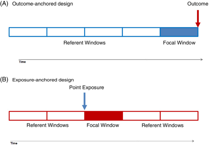
Simple representation of Self‐controlled Crossover Observational PharmacoEpidemiologic (SCOPE) study design figures using the recommended language. For simplicity, we depict a point exposure that is administered as a single dose, such as an annual influenza vaccination. Similarly, only the main observation windows of interest (focal and referent) are depicted, yet transition (induction, lag, and washout) windows and other boundaries (eg, age groups) often need to be considered. (A) Outcome‐anchored designs are typically uni‐directional in pharmacoepidemiology (as depicted), with referent window defined only prior to the outcome‐anchor. (B) Exposure‐anchored designs are typically bi‐direction meaning that referent windows before and after the exposure‐anchored focal window are considered [Colour figure can be viewed at wileyonlinelibrary.com]

BOX 2. How to Differentiate between the Main Two Groups of SCOPE Designs.

All studies start with a single point in time from which all design features relate. This point in time is commonly referred to the “index date” in cohort studies, and “outcome date” in case‐control studies. In an effort to define a common language across SCOPE studies, we use the term “anchor” to differentiate between SCOPE studies that define the primary windows of interest based on the outcome (outcome‐anchored) or exposure (exposure‐anchored). We thus encourage “outcome‐anchored” (case‐crossover [CCO], ⁵ case‐time control [CTC], ⁶ case‐case‐time control [CCTC]) ⁷ and “exposure‐anchored” (self‐controlled case‐series [SCCS]) ⁸ when describing, or differentiating between the two main groups of SCOPE study designs.

We also discourage the use of “prospective” and “retrospective;” “cohort” and “case‐control;” or “forward looking” and “backward looking.” Our motivation relates to the tendency to consider anything “retrospective” as inferior to “prospective;” and thus also the case‐control design as inferior to the cohort study design. ³⁷ This black and white mentality hampers the value of a well‐designed observational study. Although we and many others have previously categorized SCOPE designs as “prospective” and “retrospective,” or “cohort” and “case‐control;” or even “forward looking” and “backward looking;” we now encourage the adoption of “outcome‐anchored” and “exposure‐anchored” to differentiate between the main two groupings of SCOPE designs. Our recommendation is also consistent with the STrengthening the Reporting of OBservational studies in Epidemiology (STROBE) guidance document that refrains from using the terms “prospective” and “retrospective.” ³⁸

The application of SCOPE studies is increasing, yet inconsistent and ambiguous language has been used to describe methodological features that may hamper the reader's ability to understand, critique, or replicate. ¹⁰ We received funding from the International Society for Pharmacoepidemiology (ISPE) to develop guidance documents for the application and reporting of SCOPE designs. In this first paper, we start from first principles, briefly reviewing foundational concepts in causal inference, pharmacology and epidemiology that inform the design of SCOPE studies. We then introduce a common language, and SCOPE designs using published examples. Key study design features are summarized to help the reader remain mindful of potential exposure‐, outcome‐, and time‐related issues that need to be considered in the design of a SCOPE study. This document aims to provide a solid foundation and introduction for those new to SCOPE designs as well as clarify concepts and encourage a common language for experienced methodologists. This manuscript is endorsed by ISPE.

2. FOUNDATIONAL PRINCIPLES

This section briefly introduces foundational principles in causation, pharmacology and epidemiology that inform the design of SCOPE studies.

2.1. Causation and two worlds of knowledge

Table 1 contains a proposal for common language that differentiates guidance on SCOPE studies between the investigators' creation (a virtual world that we call Study), and the actual phenomena in the population (which we label Truth), based on Popper's Worlds of Knowledge, Box A1. ¹¹ Our intention is to create a common language to help clarify the distinction between biological (pharmacological) truths, and the phenomenon we wish to measure using imperfect measurement in the real‐world. For example, we encourage induction period be used exclusively based on what is known based on pharmacology, and induction window as the investigator's window of observation that is earmarked for induction in the study.

TABLE 1.

Distinction between causal and observational worlds of knowledge and proposed common language for time‐related phases

	“Truth”	“Study” or Estimation
	Causal (Biology)	Investigator driven (study contextual)
The phenomenon being studied is…	True relation (causation)	Estimated association (observation)
…which is produced by…	Biology (nature)	Measurement (investigator's design)
…which is limited or modified by…	Modifiers in human populations (pharmacology)	What is measurable and measured (data available) within the constraints of a healthcare (structural) system
…which form the bases for defining…	Hypothesized phases of the cause‐effect process	Observation windows
Time‐related phases of the phenomenon
Risk	Effect period (period of time when it is biologically plausible that exposure causes outcome, that is, exposure‐outcome effect period)	Focal window (window of interest when it is hypothesized to be biologically plausible that exposure causes outcome; temporally linked to a study design anchor) a , b
Baseline	Baseline period (period where outcome risk is determined by factors other than exposure)	Referent window (window outside the focal and transition windows chosen to estimate baseline risk when people are at biological risk for the outcome due to factors other than the exposure of interest) a
Transition time:
Induction	Induction period (period of time after a person is exposed to the drug and before the outcome is biologically possible)	Induction window (window of observation hypothesized to capture the induction period; can be modeled as a separate referent window or excluded)
Lag	Not applicable (healthcare system or data issues and thus only contextual for a SCOPE study) c	Lag window (healthcare system issue that increases or decreases exposure or outcome; can be adjusted for or excluded) c
Carryover	Carry‐over effect period (period of time after stopping the drug until drug effects on outcome risk are gone) a	Washout window (time window during which individual variation in carry‐over effect is thought to be complete; can be modeled as a separate referent window or excluded)

^aRanges between individuals, can be estimated based on population‐based incidence curves; based on current knowledge of the effect period.

^bFocal window is proposed in SCOPE studies as the “suspected” window of interest. Although exposure‐outcome risk window is more explicit, it may be technically more challenging when there is no biology to support an association, yet a safety signal is under investigation. “Hypothesized exposure‐outcome risk window” could be used, yet lengthy. “Focal” does not give value to effect, is short, and thus also strategic for inclusion in study figures and tables.

^cHealthcare system issues are not biological, rather structural issues that impact drug exposure (eg, healthy vaccine effect).

2.2. Pharmacology

SCOPE studies target drug exposures and thus design decisions are critically influenced by pharmacology (“biological truth”), including components of pharmacokinetics (what the body does to the drug), and pharmacodynamics (what the drug does to the body). Drug administration, absorption, distribution, metabolism and elimination influence the speed, intensity and duration of drug action. Therefore, pharmacologic reasoning about plausible temporal relations between causes and effects, and hypothesized durations of induction periods and carry‐over effects, influence the choice of windows of observation. The clinical crossover trial design is often used to estimate these parameters. To exemplify pharmacologic reasoning, we use the case of fluoxetine, a selective serotonin reuptake inhibitor indicated for the treatment of depression. Below, we define induction, effect, and carry‐over periods based on biological truths.

In an individual patient, the induction period is the length of time required for a drug to yield a detectable causal effect (either clinical benefit or adverse outcome). This often varies from one patient to the next and can make the population impact of a drug difficult to estimate. The induction period in a population is defined as the shortest individual induction period, labeled the minimum induction period. According to clinical trial evidence, the minimum induction period for fluoxetine's clinical benefit in major depressive disorder (ie, improvement in depressive symptoms like suicide ideation or lack of appetite) is 2‐4 weeks. ¹² However, some patients who eventually report clinical benefit from fluoxetine do not achieve a full effect until as many as 8 weeks of continuous therapy. ¹³ In contrast, the minimum induction period from first intake of fluoxetine to other common adverse outcomes, such as gastrointestinal bleeding, insomnia, nervousness or sexual dysfunction, typically occur within 2 weeks of treatment initiation. ¹² Understanding the minimum and maximum induction periods for the specific drug exposure‐outcome relationship under investigation is critical to the design of a SCOPE study.

The effect period is the period of time within which it is biologically plausible that the drug causes the outcome. The effect period immediately follows the induction period and extends from the first to the last outcome attributable to the exposure. The effect period is only meaningful in the context of a specific exposure and outcome that the “effect” relates to. The carry‐over period is the length of time when residual pharmacodynamic effects of the exposure occur after the effect period of primary interest. In a clinical crossover trial, the carry‐over effects are defined as the residual effects from exposure in the first treatment phase that are carried over to, and impact, the causal effect estimates following treatment initiation in the second treatment phase. ¹⁴ Carry‐over effects are mitigated by selecting a sufficiently long washout w. For example, fluoxetine has an elimination half‐life of 4‐6 days, and some of its active metabolites even longer. Pharmacologic methods such as dose‐response and dose‐titration studies can be used to determine the washout window that is most appropriate for an experimental crossover clinical trial of the exposure of interest. ¹⁴ For drugs that follow a first‐order pharmacokinetic model, a minimum washout window of five times the elimination half‐life of drug from plasma levels for a 97% elimination from the body is recommended. ¹⁵ However, other factors such as tissue binding and other physiologic carryover effects may last longer and be considered when selecting the washout window. ¹⁶

The next section walks through the epidemic curve and symmetry analysis to help guide the selection of observation windows in a SCOPE study.

2.3. Epidemiology

Epidemiology is the study of the occurrence, distribution and determinants of human health‐related outcomes in specified populations. ¹⁷ The epidemic curve, and related “induction curve” at the population level, can be particularly informative in defining induction, effect and washout windows in the design of a new SCOPE study. An epidemic curve provides a graphical display of the number of incident cases in an outbreak of illness plotted over time. The shape of the curve helps to inform hypotheses about the nature of the disease. The epidemic curve is most commonly used to study the course of infectious diseases, yet can inform SCOPE studies by plotting the number of incident cases relative to the start of drug exposure. For example, the self‐controlled case series (SCCS) design was motivated by an observation that risk for acute meningitis following Measles Mumps Rubella (MMR) vaccine exposure was elevated 15 to 35 days after immunization, Figure 2. ¹⁸

FIGURE 2.

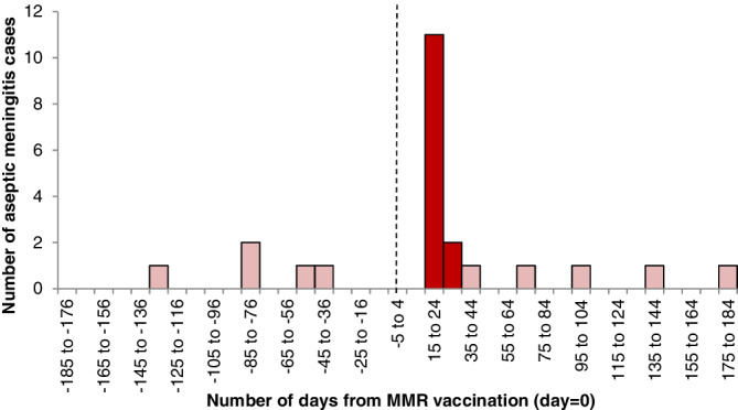
Distribution of interval (days) between Measles Mumps Rubella (MMR) vaccination (day zero, dotted line) and aseptic meningitis diagnosis. Dark bars occur within days 15 to 35, and light bars occur outside the 15 to 35 day window [Colour figure can be viewed at wileyonlinelibrary.com]

In addition to epidemic curves, sequence symmetry analysis (SSA, Box 3), may be strategically employed when little is known about the true phases of the phenomenon under study. SSA can also screen for multiple associations simultaneously. In an extreme recent analysis, more than 200 billion sequences and 3 million hypotheses were screened. ¹⁹ What SSA lacks is a formal framework for handling time‐dependent confounders or flexible handling of exposure time. Therefore, SSA may be considered a great choice for signal detection and hypothesis‐screening that can be further tested using a SCOPE design.

BOX 3. Sequence Symmetry Analysis.

The prescription sequence symmetry analysis (SSA) was introduced in 1996 as a screening tool for unknown, unsuspected associations in large datasets. ³⁹ The first paper examined whether cardiovascular medication triggered depression, represented by a proxy of incident antidepressant use. It asserted that in a population of new users of cardiovascular medication and antidepressants, an equal proportion of persons starting either drug first is expected if there is no association between cardiovascular drug use and depression. The ratio between the count of persons starting cardiovascular medication first versus starting antidepressants first estimates the incidence rate ratio. ⁴⁰ The study demonstrated symmetrical distributions of sequences, thus showing no association between cardiovascular medication and depression. Like SCOPE designs, confounders that are stable over time are eliminated by design. ³⁵ There are, however, a number of other potential explanations for an asymmetrical distribution than a causal association, such as time trends in the incidence of either drug (exposure or outcome drug), and survival bias. ³⁹ SSA can incorporate diagnoses or procedures as outcomes as well as prescription, ⁴¹ and owing to its simplicity in processing and its minimal data requirement, SSA has become popular as a screening tool in distributed networks, particularly in Asia and Australia. ⁴² In addition, if time windows of observation are restricted (eg, 30 days), the sequence ratio calculated by SSA can approximate the incidence rate ratio. Still, SSA are typically not self‐controlled as the reference is other windows that include non‐cases without a crossover component. Further research to examine the statistical performance and required assumptions for consistent estimation of SSA is encouraged.

3. OVERVIEW OF SCOPE STUDY DESIGNS

All SCOPE designs are case‐only designs at their core. Extensions may be considered hybrids as they include non‐case comparisons. Each SCOPE design uses different strategies for sampling comparison time. At the heart of each approach is the comparison of an observed frequency during focal window(s) of observation to an observed frequency during referent window(s) of observation. The observed frequency (outcome incidence or odds of exposure) during a focal (hypothesized exposure‐outcome risk) window is compared with the “usual” outcome incidence, or the “usual” odds of exposure, in referent windows that are outside the focal and transition (induction, lag and washout) windows. Depending on the specific design, experience (person‐time) from non‐cases can contribute to effect estimates to combat time‐trends or to adjust for time varying confounding. Nonetheless, at their core, all SCOPE designs compare observed frequencies (exposure or outcome) within predefined focal and referent windows, conditioned on the individual patient.

In the following sections, we adopt the proposed language in Table 1 to describe and compare SCOPE designs, Table 2. Readers are encouraged to consult a recent comparative summary for considerations of the strengths and limitations of SCOPE designs in the broader field of epidemiology. ²⁰ , ²¹ We appreciate that variation in terminology will persist in practice, yet believe that the common terminology proposed here may help in better understanding the similarities and subtle differences among alternative SCOPE approaches.

TABLE 2.

Summary of self‐controlled crossover observational pharmacoepidemiologic (SCOPE) study designs

		Relative
Design	Description a , b	Strengths	Limitations	Example
Outcome‐anchored designs
Case‐crossover (CCO) 1991	Compares exposure just before outcome (focal window), to referent window(s); may exclude transition windows and can adjust for measures of time‐varying confounders.	Efficient: only cases eligible. Typically only consider windows of observation pre‐outcome and thus does not require assumption of no outcome‐related change in exposure or observation.	Sensitive to exposure time trends (requires that exposure distribution is stationary).	Outcome: myocardial infarction 23 Exposure: cannabis Note: interview study
Case‐time control (CTC) 1995	Two CCO designs are completed; one in cases and one in a matched group of risk‐set sampled non‐cases.	Controls for exposure time trends. Can control for confounders (eg, age, sex) via matching.	Non‐case selection can be difficult and must arise from same epidemiologic study base as cases.	Outcome: myocardial infarction 25 Exposure: aripiprazole Note: newly marketed drug motivated CTC
Case‐case‐time control (CCTC) 2011	Two CCO designs are completed; one in cases and one in risk‐set sampled future cases.	Above (like CTC), and reduces selection bias in non‐cases.	Future‐case selection difficult when study short. Timing (washout) for future case eligibility can be challenging. Biased if exposure has high risk of mortality since exposure histories in future cases are among survivors and may not represent the study base.	Outcome: stroke 27 Exposure: anti‐psychotics
Exposure‐anchored design
Self‐controlled case series (SCCS) 1995 c	Compares outcome incidence in focal (exposed) windows to referent (unexposed) window(s). Typically includes all time under observation with flexible window definitions and often adjusts for measured time‐varying confounders; may exclude transition (eg, lag) windows.	Suitable for recurrent outcomes. Can control for measured time‐varying confounders.	Outcome timing should not influence subsequent exposure or observation (exceptions possible).	Exposure: measles, mumps and rubella vaccine 28 Outcome: meningitis Note: adjusts for age effect

^aWindows (focal, referent and transition [induction, lag, carry‐over]) are described in Table 1.

^bAnalyses are conditioned on the individual patient, yet when focal and referent windows match in length, aggregate data yield the same results since observation time is fixed and equivalent.

^cRelative risk estimator is similar to sequence symmetry analysis when all windows are identical.

3.1. Outcome‐anchored SCOPE designs

Outcome‐anchored designs are best thought of as “trigger” designs since they are suited to the study of transient exposures and abrupt onset outcomes, Figure 3. In pharmacoepidemiology, outcome‐anchored designs typically only consider referent windows prior to the outcome‐focal window. This is an important consideration because the probability of drug exposure often changes following an outcome. However, some outcomes, like an unknown adverse effect, would not change exposure probability and thus a bi‐directional design with reference windows pre‐ and post‐outcome can be considered. Understanding the study context and local healthcare system and norms of data under study are critical in design of any SCOPE study. In other fields, such as environmental epidemiology that consider ambient environmental exposures, referent windows before and after the outcome‐focal window are common. ²²

FIGURE 3.

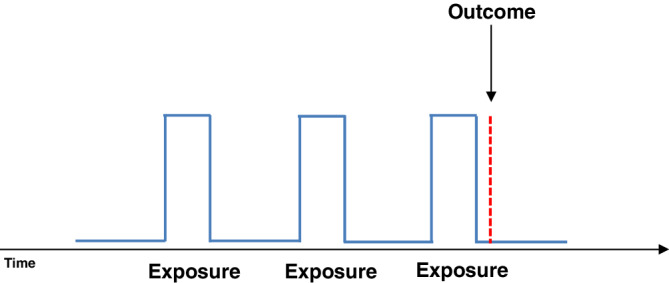
Example of a transient exposure pattern (blue solid line—exposure periods [peaks] followed by non‐exposure [valleys]) and an abrupt outcome (red broken line, short in duration with abrupt/sudden onset) [Colour figure can be viewed at wileyonlinelibrary.com]

3.1.1. Case‐crossover (CCO)

The CCO design was originally developed through an interview study investigating the relationship between myocardial infarction (MI) and various acute exposures. ⁵ The concept that control‐person selection bias could be avoided if cases served as their own controls motivated the gradual development of the design. In one of the first CCO studies, participant interviews considered medications, illicit drugs, alcohol, coffee, smoking, extreme exertion, sexual activity, anger and bereavement in the hours, days and weeks before the onset of MI. ²³ Questions were structured in several ways to explore different durations of effect periods, ranging from minutes to days between potential triggers (causal exposures) and MI onset.

The basic research question was: “Did anything unusual happen just before?” For example, among 3882 MI patients interviewed, 9 had been exposed to marijuana (now commonly referred to as cannabis) within the hour before MI symptoms, and 3 in the preceding hour. ²³ Assuming that cannabis' effect on MI risk dissipated within 1 hour, the 60 minutes before MI onset was chosen as the focal window and the preceding hour (60 to 120 minutes before MI), the referent window. This yielded a baseline (observation during the referent window) of 3 exposed patients, and thus produced a relative risk estimate of 3 (9 patients exposed in the focal window divided by 3 patients exposed in the referent window).

Since the maximum induction period was unknown, it was possible that 1 or 2 of the 3 MIs within the 60‐to‐120 minutes prior to MI were triggered by cannabis. Therefore, use of referent windows further away from the outcome were considered. In total, 25 patients reported cannabis use within the 2 to 24 hours before MI. The expected number of exposed in the 2 to 24 hours before MI observation window was thus closer to 1 per hour (25/22) than the estimate of 3 per hour from the 60‐to‐120‐minute window prior to MI.

A much larger sample of referent windows was obtained by asking patients about their usual frequency of cannabis in preceding days, weeks and months. ²³ In this analysis, each patient's data were treated as if they were an n‐of‐1 study and a stratified analysis was performed with one patient per stratum; that is, the analysis was conditioned on the individual patient. The Mantel‐Haenszel estimates of the cannabis exposure odds ratios (OR) were 4.8 (95% confidence interval [CI]: 2.9, 9.5) and 1.7 (95% CI: 0.6, 5.1) for the first and second hour before MI onset compared to other reported person‐time. The paper concluded that the risk of MI increased within an hour of cannabis (marijuana) exposure, and then dissipated. ²³

A key distinguishing feature of this broader analysis is that it is conditioned on the individual patient. CCO analytical options include Mantel‐Haenszel estimates, conditional logistic and Poisson regression. ²¹

3.1.2. Case‐time‐control (CTC)

The CTC design is an extension of the CCO that includes matched risk‐set sampled controls (ie, non‐case at the time of sampling) as well as cases in the analysis. The CTC was proposed to adjust for population level exposure time‐trends in the CCO design. ⁶ When a new drug comes to market, there is an inherent increase in the probability of exposure since the drug was not previously available. There may be a decline in use of other drugs prescribed for the same indication which are being displaced by the new drug. If not accounted for, population‐level exposure time‐trends can generate spurious associations in a CCO study. The CTC design adjusts for population‐level exposure time‐trends by comparing CCO estimates among cases to CCO estimates in time‐matched non‐cases. CTC can also adjust for other confounders such as age trends by matching on calendar time and age as an example. Non‐cases are risk‐set sampled, meaning that they are matched to cases on calendar time, and they may also be matched on age, sex or other characteristics. Because the risk‐set sampled non‐cases are matched on time to cases, observed associations among non‐cases estimate the population‐level exposure‐time trend over the same calendar time as the cases. The exposure time‐trend adjusted estimate is obtained by dividing OR_CCO(cases) by OR_{CCO(non‐cases)} and is modeled using conditional logistic regression, ⁶ with bootstrapping for confidence intervals. ²⁴ We focus on exposure time trends here, yet diagnostic trends in defining the outcome can also be adjusted using CTC.

CTC example

Population level exposure time trends are especially pronounced in new‐to‐market medical products. ²⁵ In a CCO evaluating the relationship between aripiprazole and MI, the analysis was repeated every quarter for 4 years, starting 6 months after aripiprazole entered the market. ²⁵ In the first observation window following market entry, the estimated OR_CCO(cases) was 2.7. Over time, the estimated OR declined, with OR_CCO(cases) = 1.4 by the 15th quarterly assessment. The pattern of estimated ORs in matched (age, sex, calendar time) non‐cases ran parallel to the estimates in cases; OR_{CCO(non‐cases)} = 3.1 in the first referent window and declined to 1.5 by the 15th quarterly assessment. After adjusting the CCO estimates in each observation window with the estimated exposure time‐trend in matched non‐cases, the OR_CTC were consistently null. Until the incidence of exposure reaches a steady state in the population, CCO estimates may be biased by population trends in exposure probability, and thus a CTC design is more appropriate.

3.1.3. Case‐case‐time control (CCTC)

The CCTC design is implemented in the same way as the CTC design; however, non‐cases are sampled exclusively from future cases. ⁷ , ²⁶ Because future cases are at‐risk for the event during historical person‐time, they are eligible to be sampled as non‐cases in the CCTC design. This is true in the CTC, with the distinction here that the CCTC only considers future cases. CCTC may be the only option if researchers only have access to data on cases. In addition to adjusting for population level exposure‐time trends, the CCTC has the potential to adjust for some prognosis‐related exposure‐time trends. By matching cases to imminent future cases that have not yet occurred, the prognosis‐related exposure time‐trend was mitigated in an analysis of antipsychotics and stroke. ²⁷

As with CTC, CCTC assumes similar time trends in both groups. This can be partially verified if complete population data are available, yet is often infeasible. CCTC may not be appropriate if exposure is associated with high mortality. Herein, restricting the design to exposure patterns only among cases (current and future) will underestimate the general population exposure distribution, and thus may induce selection bias. ²¹

3.2. Exposure‐anchored SCOPE designs

Exposure‐anchored SCOPE designs include SCCS and its variants (Box 4). Exposure‐anchored designs can analyze any rare, unique or recurring outcome provided the outcome is precisely documented, and recurrent event (outcome) timing is independent. When exposures are scheduled, such as childhood or seasonal vaccinations, exposure‐anchored designs are a natural choice.

BOX 4. Other Exposure‐Anchored Designs.

The self‐controlled risk interval (SCRI) and exposure crossover designs are other types of exposure‐anchored designs. In particular, the SCRI is a variant of the self‐controlled case series (SCCS) that is more restrictive about observation time. To our knowledge, the name was first used by Lee et al (2011) in an application of vaccine safety. ⁴³ SCRI is indexed on exposure, with focal and referent windows defined in relation to exposure. The analysis estimates the relative incidence during the focal (exposure) window to the referent (unexposed) window(s) using only cases identified in either window. ¹⁸ The design may be “bi‐directional” with two referent windows, one before and one after the focal window, or “uni‐directional” typically with only referent window(s) post the focal window included. Referent and focal windows need not be consecutive, for example, gaps to allow for washout or lag windows can be included, and window lengths may differ. The SCRI model typically assumes that incidence rates are constant over focal and referent windows, that is, effects of age or other temporal confounders are constant. Nonetheless, strategies to control for age and time effects by including unexposed cases like in the SCCS design or external information on daily incidence rates have been recently described. ⁴⁴ In addition, as with all SCOPE designs, stable confounders such as gender and body mass index are controlled by design.

The exposure crossover design was inspired by time series analyses of large economic changes. ⁴⁵ This outcome‐anchored design can be viewed as a highly stratified time‐series analysis with each person's experience constituting one stratum, and time zero set as the time of exposure initiation. Time segments of similar length are defined, a distinctive feature from the SCCS. To illustrate the design, we walk through an example that examined the impact of physician warnings (exposure) on subsequent motor vehicle accidents (MVA) among patients diagnosed with psychiatric conditions. ⁴⁶ It was hypothesized that the benefits of a physician warning on MVA would be immediate and last at least 1 year in duration. Time‐zero was defined as the date a patient received their first physician warning about the operation of a motor vehicle. The year immediately after time‐zero was defined as the focal window. The year prior to time‐zero was considered a lag window to avoid comparing the focal window with a time when subjects may have been acutely more likely to be in a MVA that prompted the physician warning; and was excluded from the analysis. The three years preceding the lag window were defined as three referent windows. Among 23 145 patients, the referent window accounted for 818 MVA (11.78 crashes per 1000 patients‐years) and the focal window contained 189 crashes (8.17 crashes per 1000 patient‐years), equivalent to a relative risk of 0.69 (95% CI 0.59 to 0.81) following a physician warning. In this example, the physician warning (exposure) was deemed effective. Analyses are typically aggregate and not conditioning on the individual patient and thus are deemed outside the scope of SCOPE designs. Still, analyses can be conditioned on the individual patient, for example, by using generalized estimating equations, ⁴⁵ , ⁴⁷ , ⁴⁸ and if so are similar to the SCRI.

3.2.1. Self‐controlled case series (SCCS) example

SCCS was motivated by a study of MMR vaccination in relation to aseptic meningitis. ²⁸ A plot of meningitis diagnosis relative to MMR vaccination (the induction curve) suggested a temporal association, with a spike in the number of meningitis events 15 to 35 days after vaccination, Figure 2. Unique to SCCS, referent windows typically include all observation time anchored based on calendar time. Including all observation time permits inclusion of other time‐varying confounders for adjustment, such as age boundaries. In effect, the analysis controls for time‐varying confounders, such as age and seasonal effects. Each individual's full observation time is cut into windows based on exposure status and any other measured time‐varying confounder to be accounted for, such as age group. The SCCS model then estimates the incidence, or rate, during focal (exposed) window(s) relative to referent (unexposed) window(s), accounting for observation boundaries within different windows (boundaries) of anticipated time‐varying risk. The model is fitted using conditional Poisson regression with terms for exposure status, and time‐varying confounder (eg, age groups), with allowance for each window length using offsets.

As a simple example, we use the cohort of 10 children in their second year of life discharged from hospital with viral meningitis between October 1988 and December 1991, originally published in 1993 ²⁸ and reused as an example in 2006. ¹⁸ The focal window was 15 to 35 days (inclusive) after MMR vaccination, and two age groups were defined: ages 366‐547 days and ages 548‐730 days. The estimated relative incidence for the post‐vaccination focal window was 12.04 (95%CI: 3.00‐48.26). The study concluded that MMR vaccination was associated with viral meningitis.

Use of SCCS is limited by assumptions that outcomes do not alter the probability or timing of subsequent exposure, nor affect the timing of the end of observation. Methods exist that circumvent these assumptions. For example, if a drug is specifically prescribed as a direct consequence of an outcome, such as pain relief following a motor vehicle accident; a window of time (lag window) just prior to exposure can be removed from the analysis. ²⁹ , ³⁰ We have focused here on foundational applications, and readers are encouraged to see other contributions for a non‐technical overview, ²⁹ or statistical review of extended SCCS methodology. ³⁰ SCCS provides a flexible modeling framework that can be viewed as a parent of other exposure‐anchored designs (Box 4). These include as examples, the self‐controlled risk interval that is more restrictive about observation time. In addition, the exposure crossover design has commonalities with the SCCS, yet is closer in design to a time‐series analysis. Other SCCS variants are outside the scope of this introductory guidance document. We refer readers to advanced methods employed when the original SCCS assumptions are relaxed, such as SCCS for censored, perturbed, or curtailed post‐event exposures, ³¹ and SCCS with event‐dependent observation periods. ³² Readers are also encouraged to consult other papers for guidance related to SCCS power and sample size calculations. ³³ , ³⁴

4. KEY SCOPE DESIGN CONSIDERATIONS

We categorize key considerations when designing a SCOPE study into two main areas: (1) exposure‐/outcome‐related (transient exposure and abrupt outcome), and (2) time‐related.

4.1. Exposure‐/outcome‐considerations: transient exposure and abrupt outcome

SCOPE designs are best suited to study questions of the effects of transient exposure on abrupt outcomes. The CCO design was developed to study transient exposures as depicted in Figure 3, maximizing the potential for cross‐over time between windows of exposure and non‐exposure. Only comparisons that are discordant (either exposed in the focal or referent window, yet not both) contribute to the analysis. Chronic (persistent) drug use leads to a considerable amount of concordant exposure, that is, subjects who are exposed during the focal window and all referent windows, and thus do not contribute to the overall effect estimate. Chronic (persistent) use can also induce hypersensitivity towards exposure misclassification. ³⁵ SCCS can handle long or persistent exposures albeit with lower efficiency, provided referent windows reasonably cover age groups and other time‐related confounder boundaries provided suitable unexposed cases are available. SCOPE designs are thus typically best suited to study transient exposures.

Precise timing of the outcome is critical to the application of all SCOPE studies. An accurately‐documented date of onset is needed to define outcome‐anchored focal and referent windows and avoid exposure misclassification. Ideal outcomes are well‐defined changes of state recorded with precise dates, such as asthma exacerbations that require an emergency department visit, or cardiovascular events or hip fracture that require hospitalization. Chronic outcomes without precise onset dates, such as episodes of depression or cancer development, are generally unsuitable for SCOPE designs because the outcome may not be captured within the appropriate time window, or the temporal relationship between the exposure and outcome may be unclear. Longer focal windows can be included to capture delayed diagnoses in exposure‐anchored designs (eg, MMR and autism); still outcomes with insidious onset, for example, onset prior to exposure and diagnosis after exposure, will be misclassified.

The suitability of using a SCOPE design is strongly influenced by the specific exposure‐outcome under investigation, particularly related to rapid induction period, and constant effect. Known induction periods that are immediate (<1 day), short (hours to days), or intermediate (days to weeks) based on clinical pharmacology are well suited for the design as they limit the influence of time‐varying confounding. Table 3 provides guidance (navigation) targeting the typical SCOPE study, but are not meant to be hard rules (Box 5). If time‐varying effects are suspected, different periods of suspected risk can be captured using multiple focal windows.

TABLE 3.

Summary of consideration in deciding exposure‐outcome suitability for a SCOPE study [Colour table can be viewed at wileyonlinelibrary.com]

	Level of caution	Time to onset a		Exposure course type
	Red	Long (months to years)	>4 weeks	Chronic medication
	Yellow	Intermediate (days to weeks)	4‐28 days	Long course (>14 days)
	Green	Short (hours to days)	1‐3 days	Short (≤14 days) or PRN
		Immediate (minutes to hours)	<1 day	One‐time use

Abbreviations: PRN = pro re nata, that is, as needed, taking when necessary; in theory acceptable provided can be measured accurately.

^aBased on biology, specific to exposure‐outcome under consideration.

BOX 5. Guidance (Navigation) and Not Guidelines (Hard Rules).

Our guidance document is meant to facilitate the discussion of SCOPE studies, and help frame thinking when developing a new SCOPE study. We provide some guidance with regard to different considerations, yet recognize that in different contexts, assumptions may be stretched and provide correct inference. Indeed, methodological innovation is only possible by pushing boundaries, “breaking rules,” trying and testing new things. We thus provide guidance (navigation) to help in considering different study design features, rather than endorsing strict adherence.

4.2. Time‐related issues and the fallacy of reverse causality

SCOPE studies control for time‐invariant confounding, such as genetics, by design. However, like any observational study, SCOPE designs need to consider time‐varying risk factors (confounders). ³⁶ These issues have been covered throughout this document with emphasis on those that tap into the likelihood (timing) of exposure relative to outcome, examples are provided in Box 6. Of particular note is the concept of reverse causality. Reverse causality is a fallacy that occurs when an apparent association between A to B is explained by a causal link in the opposite direction, from B to A. Reverse causality is frequently encountered in epidemiologic research and may include aspects of selection (eg, indication or contra‐indication) and information (measurement, ie, the validity of the timing of disease outcome or exposure), Box 7. Careful consideration of outcome timing and whether or not exposure likelihood changes following the outcome under consideration are important when the design includes observation time post‐outcome. Time‐related changes may need to be controlled for by design, excluded (eg, lag window), or adjusted for in analysis. In the context of permanent contra‐indication following an outcome, comparison should only be made between windows prior to outcome (outcome‐anchored design) or after exposure initiation (exposure‐anchored designs).

BOX 6. Examples of Time‐Related Issues That Need to be Considered.

1. Population‐level exposure time trends

   It is critical to consider the healthcare system and data available for analysis. The following lists example population‐level exposure time trends to consider:

   • New drug to market (increase in use of new drug that may also displace older drugs)
   • Drug withdrawal from market
   • Drug formulary change
   • Change in clinical practice guideline recommendations for pharmacotherapy
   • Deprescribing initiatives
   • Regulatory changes (eg, pharmacist permitted to dispense drugs without prescriptions during the COVID‐19 pandemic)
2. Patient‐level exposure time trends

   • Exposure is less common during periods of illness (eg, vaccines for prevention)
   • Patients with increasing frailty/functional decline may seek healthcare more often, and thus more likely be exposed to a variety of healthcare interventions and medications just prior to the outcome
   • When outcome carries a high mortality risk, post‐outcome referent windows to identify exposure may be unlikely
   • When exposure is associated with mortality, application of the case‐case time‐control design may underestimate exposure trends in the base population since exposure histories are limited to future cases (survived to become a case)
   • Exposure misclassification during hospitalization
   • Contraindication to exposure post‐outcome
   • Exposure‐level changes during pregnancy
3. Population‐level outcome time trends

   • Change in clinical practice guidelines that impact outcome definition
   • Change in medical claim coding practices, for example, from ICD‐9 to ICD‐10
4. Patient‐level outcome time trends

   • Calendar time or season, for example, falls risk and thus fracture risk increases in some regions during the winter due to the hazards of ice and snow
   • Age trends, for example, risk of cardiovascular events increase with age

BOX 7. Reverse Causation (Fallacy of Reverse Causality).

Reverse causation results in a fallacy in the data related to indication, contra‐indication or delayed diagnosis. Some examples of the mechanisms resulting in reverse causation are:

1. Initial symptoms of a condition are misinterpreted (information [measurement of when disease diagnosed, sometimes referred to as protopathic bias] or selection [indication] bias)

   • an apparent association between proton pump inhibitors (PPIs) and pancreatic cancer is explained by the earliest symptoms of the cancer being interpreted as acid‐related dyspepsia and treated with PPI. Later, the cancer diagnosis is established. Since use of PPIs typically precede the cancer diagnosis, an apparent association is generated when in reality, the causality is in the opposite direction, from pancreatic cancer to PPI use.
2. Exposure initiated due to early signs of the risk or concern for an outcome (selection [indication] bias)

   • an apparent association between PPI use and reflux esophagitis may be explained by PPI being prescribed in primary care for indeterminate dyspepsia. Later the patient is referred for diagnostic work‐up, and a diagnosis of reflux esophagitis is established. The apparent association is PPI causes reflux esophagitis, while the true causality is in the opposite direction. This is an example of information bias since the true diagnosis (outcome) is delayed/initially misclassified.
3. Exposure likelihood changes post‐outcome (selection [contra‐indication] bias)

   • an apparent association between a drug and outcome can be explained by the switch from the weaker drug to more potent drug following healthcare event (eg, outcome or hospitalization). The apparent association that the weaker drug causes the outcome can be explained from the switch post‐outcome, when the switch is because of the outcome.
4. Outcome likelihood is less likely pre‐exposure (selection [contraindication, or more specifically: healthy vaccine] bias)

   • vaccination for prevention is usually postponed if children are sick and thus there is often low incidence of the outcome immediately prior to vaccine exposure. Care must be taken to remove the observation window immediately prior to vaccination (lag window) otherwise estimates of relative incidence will be inflated.

A worksheet is provided in Data S1 to facilitate critical thinking in the design and review of SCOPE studies.

5. SUMMARY

SCOPE studies are methodological innovations initially developed in the 1990s with more recent extensions that complement the traditional cohort and case‐control studies. These designs are grouped into two main types, exposure‐anchored or outcome‐anchored, based on how the investigator anchors the timing of windows of observations. SCOPE designs use the individual's own experience as reference, thereby controlling for time‐invariant (stable) within‐person confounders, such as a patient's genetics. These designs are thus conceptually similar to the crossover clinical trial. A distinguishing feature of these designs is that analyses are conditioned on the individual patient. Thus, SCOPE designs can estimate the counterfactual, provided comparative windows of observation are indeed exchangeable. At their core, SCOPE designs are case‐only, yet extensions may use non‐case time to control for population time trends or time‐varying confounders such as age. In addition, these designs can adjust for within‐person time‐varying confounding, such as a person's age when disease risk varies with age, or calendar time when a disease varies by season. This foundational document introduces the main types of SCOPE studies and the key issues that need to be considered when designing a SCOPE study; these relate to exposure (transient is ideal), outcome (abrupt is ideal), the exposure‐outcome association (rapid induction and constant effects are ideal), and time‐trends. The main weakness of SCOPE studies relates to time‐dependent confounding and measurement of exposure and outcome. However, these limitations are not unique to SCOPE studies and are important considerations in any observational setting, including cohort and case‐control designs. In conclusion, SCOPE studies are an important design in pharmacoepidemiology that like all studies require careful consideration related to time trends and windows of observation.

CONFLICTS OF INTEREST

SMC, MM, JACD, HJW, KNH, MT, GPC and JH report no conflicts of interest. JJG has received salary support from grants from Eli Lilly and Company and Novartis Pharmaceuticals Corporation to Brigham and Women's Hospital and was a consultant to Optum Inc., all for unrelated work. SVW has received salary support from investigator‐initiated grants to Brigham and Women's Hospital from Boehringer Ingelheim, Novartis Pharmaceuticals and Johnson & Johnson.

ETHICS STATEMENT

Authors declare that no ethical approval was needed.

SPONSORS

This guidance report was supported by a manuscript proposal grant to Dr. Cadarette from the International Society for Pharmacoepidemiology (ISPE).

PRIOR PRESENTATIONS

Earlier versions of this guidance document were presented as a symposium at the International Society for Pharmacoepidemiology (ISPE)'s Annual Meeting, May 2017 in Montreal, and as a pre‐conference course at the ISPE Mid‐Year Meeting, April 2018 in Toronto.

Supporting information

DATA S1 Supporting information

APPENDIX A.

A.1.

BOX A1. Philosophical Understanding of Causation—Popper's Worlds of Knowledge.

1.

In this foundational paper, we differentiate between the investigators' creation; a virtual world that we call Study; and the actual phenomena in the population, which we label Truth, Table 1. Aspects of the causal, biological, Truth that we want to understand are juxtaposed with corresponding aspects of the Study—the epidemiologist's “camera” for making observations. ⁴⁹ The Truth corresponds to Karl Popper's concept of World 1; the real world of matter and energy, molecules and motions, organisms and disease processes, that we observe and try to understand. World 2 comprises mortal and highly fallible knowledge in organisms' nervous systems; including epidemiologists' individual perceptions, opinions, ideas, attitudes and skills that we use to design and conduct a study. In this foundational document, the term Study refers to the study's manifestation in Popper's concept of World 3: Objective Knowledge, meaning recorded knowledge, a special part of which is called the “Evidence” in the literature on Evidence‐Based Medicine.

These distinctions are helpful for clarifying concepts and terminology about things in World 1, a true causal relationship that can never be fully known with certainty; World 2 our personal fallible perceptions of truth, evidence and methodology that go into planning a SCOPE study; and World 3, the current state of imperfect evidence about that relationship, and methods for adding to the evidence.

We use the term period to refer to time‐related biological phases of the true cause‐effect process (summarized under pharmacology), and the term window to refer to investigators' choices of time‐related intervals in which to observe phenomena.

Pharmacology may be thought of studying drug effects in the causal world (truth), whereas epidemiology may be considered studying drug effects in the observational world (study). Reducing our fallibility is the immediate purpose of this document. The long‐term goal is to reduce imperfections in the evidence.

Cadarette SM, Maclure M, Delaney JAC, et al. Control yourself: ISPE‐endorsed guidance in the application of self‐controlled study designs in pharmacoepidemiology. Pharmacoepidemiol Drug Saf. 2021;30:671–684. 10.1002/pds.5227

REFERENCES

- 1. Public Policy Committee, International Society of Pharmacoepidemiology . Guidelines for good pharmacoepidemiology practice (GPP): guidelines for good pharmacoepidemiology practice. Pharmacoepidemiol Drug Saf. 2016;25:2‐10. 10.1002/pds.3891. [DOI] [PubMed] [Google Scholar]
- 2. Schneeweiss S, Avorn J. A review of uses of health care utilization databases for epidemiologic research on therapeutics. J Clin Epidemiol. 2005;58:323‐337. 10.1016/j.jclinepi.2004.10.012. [DOI] [PubMed] [Google Scholar]
- 3. MacMahon S, Collins R. Reliable assessment of the effects of treatment on mortality and major morbidity, II: observational studies. Lancet. 2001;357:455‐462. 10.1016/S0140-6736(00)04017-4. [DOI] [PubMed] [Google Scholar]
- 4. Schneeweiss S. Sensitivity analysis and external adjustment for unmeasured confounders in epidemiologic database studies of therapeutics. Pharmacoepidemiol Drug Saf. 2006;15:291‐303. 10.1002/pds.1200. [DOI] [PubMed] [Google Scholar]
- 5. Maclure M. The case‐crossover design: a method for studying transient effects on the risk of acute events. Am J Epidemiol. 1991;133:144‐153. [DOI] [PubMed] [Google Scholar]
- 6. Suissa S. The case‐time‐control design. Epidemiology. 1995;6:248‐253. [DOI] [PubMed] [Google Scholar]
- 7. Wang S, Linkletter C, Maclure M, et al. Future cases as present controls to adjust for exposure trend bias in case‐only studies. Epidemiology. 2011;22:568‐574. 10.1097/EDE.0b013e31821d09cd [DOI] [PMC free article] [PubMed] [Google Scholar]
- 8. Farrington CP. Relative incidence estimation from case series for vaccine safety evaluation. Biometrics. 1995;51:228‐235. [PubMed] [Google Scholar]
- 9. Tse A, Tseng HF, Greene SK, Vellozzi C, Lee GM. Signal identification and evaluation for risk of febrile seizures in children following trivalent inactivated influenza vaccine in the Vaccine Safety Datalink Project, 2010–2011. Vaccine. 2012;30:2024‐2031. 10.1016/j.vaccine.2012.01.027. [DOI] [PubMed] [Google Scholar]
- 10. Consiglio GP. Diffusion of methodological innovation in pharmacoepidemiology: self‐controlled study designs [thesis]. TSpace, University of Toronto: 2015;March. https://tspace.library.utoronto.ca/handle/1807/69078. [Google Scholar]
- 11. Popper KR. Three worlds. Mich Q Rev. 1979;28(1):1‐23. [Google Scholar]
- 12. Kennedy SH, Lam RW, McIntyre RS, et al. Canadian Network for Mood and Anxiety Treatments (CANMAT) 2016 clinical guidelines for the management of adults with major depressive disorder: section 3. Pharmacological treatments. Can J Psychiatr. 2016;61:540‐560. 10.1177/0706743716659417 [DOI] [PMC free article] [PubMed] [Google Scholar]
- 13. Schweitzer E, Rickels K, Amsterdam J. What constitutes an adequate antidepressant trial of fluoxetine? J Clin Psychiatry. 1990;51:8‐11. [PubMed] [Google Scholar]
- 14. Cleophas TJM. Carryover bias in clinical investigations. J Clin Pharmacol. 1993;33:799‐804. 10.1002/j.1552-4604.1993.tb01954.x. [DOI] [PubMed] [Google Scholar]
- 15. Ito S. Pharmacokinetics 101. Paediatr Child Health. 2011;16:535‐536. [DOI] [PMC free article] [PubMed] [Google Scholar]
- 16. Niazi S. Handbook of Bioequivalence Testing. London, UK: CRC Press; 2007. [Google Scholar]
- 17. Porta M, ed. A Dictionary of Epidemiology|. 6th ed. Oxford: Oxford University Press; 2014. [Google Scholar]
- 18. Whitaker HJ, Paddy Farrington C, Spiessens B, Musonda P. Tutorial in biostatistics: the self‐controlled case series method. Stat Med. 2006;25:1768‐1797. 10.1002/sim.2302. [DOI] [PubMed] [Google Scholar]
- 19. Hallas J, Wang SV, Gagne JJ, Schneeweiss S, Pratt N, Pottegård A. Hypothesis‐free screening of large administrative databases for unsuspected drug‐outcome associations. Eur J Epidemiol. 2018;33:545‐555. 10.1007/s10654-018-0386-8. [DOI] [PubMed] [Google Scholar]
- 20. Baker MA, Lieu TA, Li L, et al. A vaccine study design selection framework for the postlicensure rapid immunization safety monitoring program. Am J Epidemiol. 2015;181:608‐618. 10.1093/aje/kwu322 [DOI] [PubMed] [Google Scholar]
- 21. Mostofsky E, Coull BA, Mittleman MA. Analysis of observational self‐matched data to examine acute triggers of outcome events with abrupt onset. Epidemiology. 2018;29:804‐816. 10.1097/EDE.0000000000000904 [DOI] [PMC free article] [PubMed] [Google Scholar]
- 22. Carracedo‐Martínez E, Taracido M, Tobias A, Saez M, Figueiras A. Case‐crossover analysis of air pollution health effects: a systematic review of methodology and application. Environ Health Perspect. 2010;118:1173‐1182. 10.1289/ehp.0901485. [DOI] [PMC free article] [PubMed] [Google Scholar]
- 23. Mittleman MA, Lewis RA, Maclure M, Sherwood JB, Muller JE. Triggering myocardial infarction by marijuana. Circulation. 2001;103:2805‐2809. 10.1161/01.CIR.103.23.2805. [DOI] [PubMed] [Google Scholar]
- 24. Delaney JAC, Suissa S. The case‐crossover study design in epidemiology. In: Borgan Ø, Breslow N, Chatterjee N, Gail MH, Scott A, Wild CJ, eds. Handbook of Statistical Methods for Case‐Control Studies. 1st ed. London: Chapman and Hall/CRC; 2018:117‐131. 10.1201/9781315154084-7 [DOI] [Google Scholar]
- 25. Wang SV, Schneeweiss S, Maclure M, Gagne JJ. “First‐wave” bias when conducting active safety monitoring of newly marketed medications with outcome‐indexed self‐controlled designs. Am J Epidemiol. 2014;180:636‐644. 10.1093/aje/kwu162 [DOI] [PMC free article] [PubMed] [Google Scholar]
- 26. Wang SV, Gagne JJ, Glynn RJ, Schneeweiss S. Case‐crossover studies of therapeutics: design approaches to addressing time‐varying prognosis in elderly populations. Epidemiology. 2013;24:375‐378. 10.1097/EDE.0b013e31828ac9cb. [DOI] [PMC free article] [PubMed] [Google Scholar]
- 27. Wang S, Linkletter C, Dore D, Mor V, Buka S, Maclure M. Age, antipsychotics, and the risk of ischemic stroke in the veterans health administration. Stroke. 2012;43:28‐31. 10.1161/STROKEAHA.111.617191. [DOI] [PubMed] [Google Scholar]
- 28. Miller E, Goldacre M, Pugh S, et al. Risk of aseptic meningitis after measles, mumps, and rubella vaccine in UK children. Lancet Lond Engl. 1993;341:979‐982. [DOI] [PubMed] [Google Scholar]
- 29. Petersen I, Douglas I, Whitaker H. Self controlled case series methods: an alternative to standard epidemiological study designs. BMJ. 2016;i4515. 10.1136/bmj.i4515. [DOI] [PubMed] [Google Scholar]
- 30. Whitaker HJ, Ghebremichael‐Weldeselassie Y. Self‐controlled case series methodology. Annu Rev Stat Appl. 2019;6:241‐261. 10.1146/annurev-statistics-030718-105108. [DOI] [Google Scholar]
- 31. Farrington CP, Whitaker HJ, Hocine MN. Case series analysis for censored, perturbed, or curtailed post‐event exposures. Biostatistics. 2008;10:3‐16. 10.1093/biostatistics/kxn013. [DOI] [PubMed] [Google Scholar]
- 32. Farrington CP, Anaya‐Izquierdo K, Whitaker HJ, Hocine MN, Douglas I, Smeeth L. Self‐controlled case series analysis with event‐dependent observation periods. J Am Stat Assoc. 2011;106:417‐426. 10.1198/jasa.2011.ap10108 [DOI] [Google Scholar]
- 33. Musonda P, Paddy Farrington C, Whitaker HJ. Sample sizes for self‐controlled case series studies. Stat Med. 2006;25:2618‐2631. 10.1002/sim.2477. [DOI] [PubMed] [Google Scholar]
- 34. Li R, Stewart B, Weintraub E. Evaluating efficiency and statistical power of self‐controlled case series and self‐controlled risk interval designs in vaccine safety. J Biopharm Stat. 2016;26:686‐693. 10.1080/10543406.2015.1052819. [DOI] [PMC free article] [PubMed] [Google Scholar]
- 35. Hallas J, Pottegård A. Use of self‐controlled designs in pharmacoepidemiology. J Intern Med. 2014;275:581‐589. 10.1111/joim.12186. [DOI] [PubMed] [Google Scholar]
- 36. Sterne JA, Hernán MA, Reeves BC, et al. ROBINS‐I: a tool for assessing risk of bias in non‐randomised studies of interventions. BMJ. 2016;i4919. 10.1136/bmj.i4919. [DOI] [PMC free article] [PubMed] [Google Scholar]
- 37. Vandenbroucke JPA. Prospective versus retrospective: what's in a name? BMJ. 1991;302:249‐250. [DOI] [PMC free article] [PubMed] [Google Scholar]
- 38. Vandenbroucke JP, Pocock SJ, Poole C, Schlesselman JJ, Egger M. Strengthening the Reporting of Observational Studies in Epidemiology (STROBE): Explanation and Elaboration. Int J Surg: 2014;12(12):1500‐1524. [DOI] [PubMed] [Google Scholar]
- 39. Hallas J. Evidence of depression provoked by cardiovascular medication: a prescription sequence symmetry analysis. Epidemiology. 1996;7:478‐484. [PubMed] [Google Scholar]
- 40. Wahab IA, Pratt NL, Wiese MD, Kalisch LM, Roughead EE. The validity of sequence symmetry analysis (SSA) for adverse drug reaction signal detection. Pharmacoepidemiol Drug Saf. 2013;22:496‐502. 10.1002/pds.3417. [DOI] [PubMed] [Google Scholar]
- 41. Tsiropoulos I, Andersen M, Hallas J. Adverse events with use of antiepileptic drugs: a prescription and event symmetry analysis. Pharmacoepidemiol Drug Saf. 2009;18(6):483‐491. [DOI] [PubMed] [Google Scholar]
- 42. Lai EC‐C, Pratt N, Hsieh C‐Y, et al. Sequence symmetry analysis in pharmacovigilance and pharmacoepidemiologic studies. Eur J Epidemiol. 2017;32:567‐582. 10.1007/s10654-017-0281-8. [DOI] [PubMed] [Google Scholar]
- 43. Lee GM, Greene SK, Weintraub ES, et al. H1N1 and seasonal influenza vaccine safety in the vaccine safety datalink project. Am J Prev Med. 2011;41:121‐128. 10.1016/j.amepre.2011.04.004 [DOI] [PubMed] [Google Scholar]
- 44. Li L, Kulldorff M, Russek‐Cohen E, Kawai AT, Hua W. Quantifying the impact of time‐varying baseline risk adjustment in the self‐controlled risk interval design: SCRI design with time‐varying baseline risks. Pharmacoepidemiol Drug Saf. 2015;24:1304‐1312. 10.1002/pds.3885. [DOI] [PubMed] [Google Scholar]
- 45. Redelmeier DA. The exposure‐crossover design is a new method for studying sustained changes in recurrent events. J Clin Epidemiol. 2013;66:955‐963. 10.1016/j.jclinepi.2013.05.003. [DOI] [PubMed] [Google Scholar]
- 46. Lustig AJ, Kurdyak PA, Thiruchelvam D, Redelmeier DA. Physician warnings in psychiatry and the risk of road trauma: an exposure crossover study. J Clin Psychiatry. 2016;77:e1256‐e1261. 10.4088/JCP.15m10224. [DOI] [PubMed] [Google Scholar]
- 47. Hanley JA. Statistical analysis of correlated data using generalized estimating equations: an orientation. Am J Epidemiol. 2003;157:364‐375. 10.1093/aje/kwf215 [DOI] [PubMed] [Google Scholar]
- 48. Redelmeier DA, May SC, Thiruchelvam D, Barrett JF. Pregnancy and the risk of a traffic crash. Can Med Assoc J. 2014;186:742‐750. 10.1503/cmaj.131650. [DOI] [PMC free article] [PubMed] [Google Scholar]
- 49. Maclure M, Schneeweiss S. Causation of bias: the episcope. Epidemiology. 2001;12:114‐122. 10.1097/00001648-200101000-00019. [DOI] [PubMed] [Google Scholar]
Associated Data
This section collects any data citations, data availability statements, or supplementary materials included in this article.
Supplementary Materials