Early Detection of Alzheimer's Disease Based on Clinical Trials, Three-Dimensional Imaging Data, and Personal Information Using Autoencoders

Abstract

Background:

A timely diagnosis of Alzheimer's disease (AD) is crucial to obtain more practical treatments. In this article, a novel approach using Auto-Encoder Neural Networks (AENN) for early detection of AD was proposed.

Method:

The proposed method mainly deals with the classification of multimodal data and the imputation of missing data. The data under study involve the MiniMental State Examination, magnetic resonance imaging, positron emission tomography, cerebrospinal fluid data, and personal information. Natural logarithm was used for normalizing the data. The Auto-Encoder Neural Networks was used for imputing missing data. Principal component analysis algorithm was used for reducing dimensionality of data. Support Vector Machine (SVM) was used as classifier. The proposed method was evaluated using Alzheimer's Disease Neuroimaging Initiative (ADNI) database. Then, 10fold crossvalidation was used to audit the detection accuracy of the method.

Results:

The effectiveness of the proposed approach was studied under several scenarios considering 705 cases of ADNI database. In three binary classification problems, that is AD vs. normal controls (NCs), mild cognitive impairment (MCI) vs. NC, and MCI vs. AD, we obtained the accuracies of 95.57%, 83.01%, and 78.67%, respectively.

Conclusion:

Experimental results revealed that the proposed method significantly outperformed most of the stateoftheart methods.

Introduction

Alzheimer's disease (AD) is one of the neurodegenerative brain dysfunctions frequently observed in elderly people. Amyloid plaques, neurofibrillary tangles, and histopathologic changes are commonly used for characterizing this disease from dementia because of their association with neuronal loss and reduction in volume of the brain.[1] This disease starts with loss of memory, progressively, in the following cognitive functions, getting worse, and worse until patients lose their ability to remember recent events, and cannot recognize very familiar persons and things. In the upcoming years, the dominance and severity of this disease is expected to rise[2] due to the regular growth of the aged population all over the world. In this sequel, it could be one of the major causes of death in the near future. Nevertheless, there is not any thorough treatment for AD yet. Thus, early diagnosis of AD could be of a considerable help in increasing the patients' survival rate. As such, many biomedical imaging techniques for early detection of AD are well developed and employed by the researchers including magnetic resonance imaging (MRI),[3,4,5] positron emission tomography (PET),[6,7] and others such as cerebrospinal fluid (CSF),[8] AD Assessment Scale–Cognitive behavior section,[9] and Mini-Mental State Examination (MMSE).[9]

Machine learning techniques are used on medical images of the brain for automatic diagnosis of AD in many studies such as Acharya et al. in[10] diagnosed AD with an accuracy of 99.48% on 33 patients and subjects using MRI images from the Harvard Brain Atlas. Wang et al. in[11] using 196 MRI images half train and half test, employed convolutional NN for a deep learning method for distinguishing AD from normal controls (NCs) and achieved 97.65% accuracy. In addition, various approaches based on structural images have been proposed. Almost all of these CAD systems have three main steps, which are preprocessing, feature extraction, and classification. The procedure of the first step sets different images from different individuals, with brains of different sizes and shapes, at a comparable condition. At the second step, feature extraction algorithm converts the input data into small vectors.[12] All the relevant information of the input data must be in these vectors. The classifier determines that the vectors are more similar to mild cognitive impairment (MCI) patient vectors, to AD patient vectors, or to NC vectors. Richer information can help to improve diagnostic accuracy.

Metrics of the entorhinal cortex have been used to discriminate AD patients and NCs,[13] but most of the studies on AD have used manual segmentation of the hippocampus in MR images.[14,15,16] These studies have high efficiency in distinguishing between AD patients and NCs. Automatic hippocampal volume-measuring methods almost have equal results.[17,18] Hippocampal volumes and entorhinal cortex metrics seem to be equally accurate in distinguishing between AD patients and NCs.[19] Single tissue such as the hippocampus alone is not enough for the accurate diagnosis of the disease, and the combination of different structures has proven to be more useful for distinguishing AD patients from NCs.[20] Therefore, using multivariate approaches, many variables simultaneously and observation of the essential patterns of different regions of the brain data can be analyzed. There were different techniques such as principal component analysis (PCA), artificial neural networks, fuzzy neural networks, partial least square, and support vector machine (SVM) to classify MRI data according to prior studies. Here, the SVM method utilizing autoencoder has been used for data analysis.

Combined techniques can use different modalities including MRI, PET, and other neurological data to diagnose AD/MCI patients from healthy people.[21,22,23,24] Lahmiri and Shmuel[25,26] used MRI images from the AD neuroimaging initiative (ADNI) dataset for distinguishing AD patients from NCs. They reported complete performance (100% accuracy) in distinguishing between the two groups. Maqsood et al.[21] reported a multiple classification using transfer learning on AD, while Beheshti et al.[27] classified AD vs. NC with a great rate of accuracy using only MRI data. Spasov et al.[28] classified progressive MCI vs. static MCI using combined MRI, APOe4 genetic, and cognitive measures include. Furthermore, automatic diagnosis of MCI using electroencephalogram spectral features is done.[29]

In this study, the feature extraction and feature combination were often performed independently. As investigated in the previous studies, there exist inherent relations between modalities of MRI and PET.[30] Thus, finding the shared feature representation which combines the complementary information from modalities (e.g., PET, MRI, and CSF) is useful to enhance the diagnosis performance of AD and MCI patients from NCs.

The data used in this article are presented in the next section, preprocessing technique, feature selection, description of proposed methodology, and classification methods, which are shown in the “Experiments and Results” section. Proposed method and the experimental results in this work are provided in the”Discussion” section. The conclusions are presented in the final section.

The dataset was used in this article, which was obtained from various sources associated with the ADNI database (adni.loni.usc.edu). The foremost usages of determining sensitive and specific biomarkers associated with the early progression include the development of new treatments with monitoring their effectiveness and the reduction in the time and cost of clinical experiments. Moreover, it should be noted that the obtained dataset was compliant only with the first examination of each patient involving 705 patients' images.

The demographic data of patients are summarized in Table 1. The MRI and positron emission tomography (PET) data were downloaded from the ADNI. A detailed description of PET protocols and acquisition can be found at www.adni-info.org. The CSF biomarker,[8,31] the personal information, and the MMSE scores were downloaded from the ADNI website since July 2015.

Table 1.

Data of patients in the Alzheimer’s disease neuroimaging initiative database

	Count	Male	Female	Married	Widowed	Divorced	Never married	Average of age	Average of MMSE
AD	156	76	80	127	18	8	3	74.89	23.32
NC	211	110	101	142	38	17	14	75.91	29.13
MCI	338	215	123	269	39	24	6	74.51	27.05
Total	705	401	304	538	95	49	23	75.01	26.85

AD – Alzheimer’s disease; NC – Normal control; MIC – Mild cognitive impairment; MMSE – Mini-Mental State Examination

Materials and Methods

Feature extraction

The features of MRI images were extracted based on regions of interest (ROIs). The MMSE scores, PET extracted features, and CSF measures are obtained from the ADNI database. The volume and the voxel values of specific regions such as hippocampus, entorhinal cortex, temporal, parietal lobes, and ventricles are the main affected regions of the brain on which AD attacks and destroys several brain cells during the early stages of its progression.[32] Figure 1 represents MRI samples of NCs and AD patients. The figure shows decreased gray matter volume in an AD patient compared.

Figure 1.

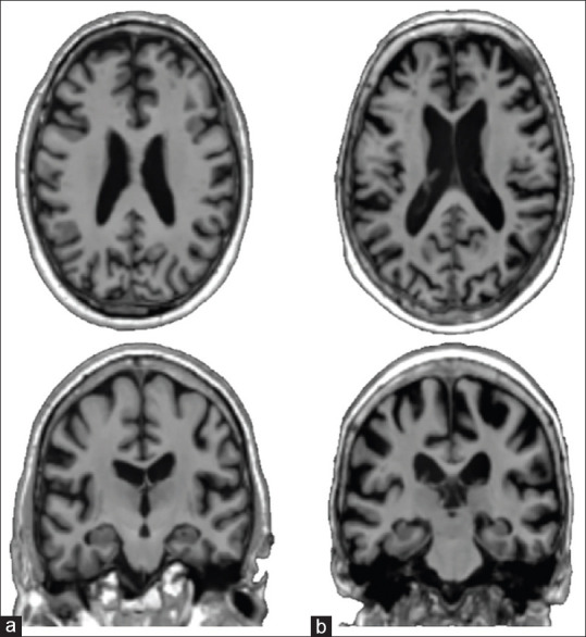
Magnetic resonance imaging sample, (a) a normal control and (b) a Alzheimer's disease patient

In Figure 2, the segmented brain and corresponding labels containing the aforementioned ROIs are demonstrated. The ROIs included candidate input variables for diagnosis of Alzheimer's disease, measures of regional cortical thickness.[33] The ROI voxels' values and their volumes for every MRI and PET images were extracted using SPM toolbox in MATLAB. Overall, the features MMSE, personal information, CSF biomarkers, and PET and MRI data have been used to classify NCs and MCI and AD patients.

Figure 2.

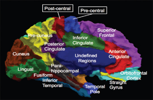
Sub-regions of medial surface of the human cerebral cortex

Autoencoder neural networks

An autoencoder is a neural network consisting of at least three layers: an input layer, a hidden layer, and an output layer, as shown in Figure 3 (it can have multiple hidden layers though). The Neurons of the first layer represent the original input vector. The hidden layer can be seen as a high-level representation of the previous layer. The output layer is a specific representation of the input layer with the same dimensionality as the input one.[34,35] The input layer sends features from MRI, PET, and CSF data to the hidden layers. Then, the hidden layer performs nonlinear transformations on the received data and imposes some optimization procedures to reconstruct the original instance.

Figure 3.

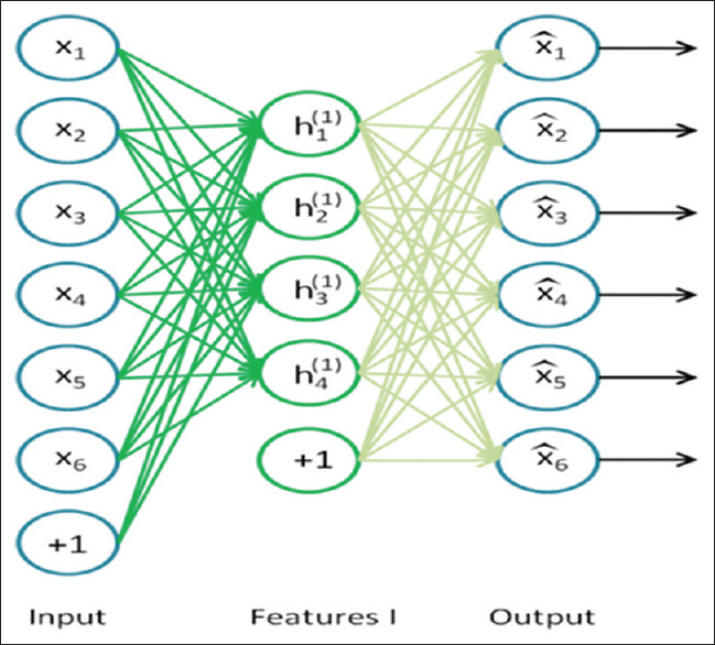
An autoencoder having an input layer (encode), one hidden layer, and an output layer (decode)

The activation signals are propagated forward through the network which can be considered sigmoid function or hyperbolic tangent function to introduce nonlinearity for the network for complex relationships of the model.[36] By modifying the number of neurons at each hidden layer, we were able to perform the feature dimensionality reduction. The hidden layers of sparse autoencoder will be trained one at a time, and they will be stacked to form a complete neural network by removing the temporary output layer.[37]

Classification and evaluation

One of the most common techniques for dimension reduction of data is PCA. It maps the data to a lower dimension while maintaining the variance of the data. Reduction of used storage space and computation time and elimination of correlated features are advantages of using PCA. Loosing some information of the original data, failing when covariance are not enough to define data, and indetermination of the number of principal components to keep information of data are disadvantages of using it.

SVM is one of the widely used classification algorithms in neuroimaging data.[4,38,39] Classification efficiency of SVM in training high dimensional data has been proven. Moreover, SVM has been applied to voice activity detection, pattern recognition, classification, and regression analysis.[40,41] It is used to separate a set of training data with a hyperplane that is maximally distant from the two classes. SVM is the most common and efficient classifier in binary classification. Here, SVM was used to distinguish between AD and MCI patients and NCs, pairwise.

One of the well-known evaluation measures is accuracy rate of a classification procedure, which computes the ratio between correctly classified samples and total samples. Sensitivity and specificity are the other evaluation metrics. Other widely used parameters to describe the performance of diagnostic procedures are positive predictive value (PPV), negative predictive value (NPV), area under the curve (AUC), and receiver operating characteristic (ROC). The accuracy, sensitivity, specificity, PPV, and NPV are defined as below:

Where TP stands for the number of true positives (number of correctly classified AD or MCI patients). TN is the number of true negatives (number of correctly classified NC or MCI patients). FP stands for the number of false positives (number of NCs classified as AD or MCI patients or MCI classified as AD). FN is the number of false negatives (number of AD or MCI patients classified as MCI patients or NCs, wrongly).

Specificity and sensitivity were used to evaluate the rate of actual positives or negatives, which were identified correctly, for example, the percentage of AD or MCI patients or NCs. These measures show the detection capability of a method between AD, MCI, and NC patterns. These metrics were measured using K-fold cross-validation (with k = 10). K-fold cross-validation has been used to audit the partial accuracy of different multivariate analysis methods applied to the segmentation of brain dementia from AD. In the K-fold method, 10 selected sets of AD and MCI patients and NCs are sampled randomly. It holds out a set for testing purposes and trains the classifier with the remaining sets. This has to be done for all 10 sets, and an average value of the evaluation parameters is calculated. We train the SVM classifier until the cross-validation loss (error) should be less or equal to 0.05.

Proposed method

A method for early detection of AD was proposed. Data normalization, replacement of missing data using best possibility, and classification of AD, NC and MCI using SVM classifier on multimodal data (MRI and PET images of brain and CSF biomarker, MMSE scores, age, education, gender, and marriage information), and finally, reducing dimension of input data was the stages of the proposed method. Before doing so, proper features of the interested area of the images had to be extracted. Then, missing data were replaced using autoencoder (a type of neural network). Finally, classification was done using a SVM classifier. Figure 4 displays the diagram of the proposed algorithm of this article.

Figure 4.

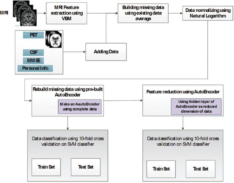
Diagram of proposed method

To distinguish between AD and MCI patients and NCs, a method for the integration and classification of the baseline MRI, PET, MMSE scores, personal information, and CSF data has been developed. The composite of extracted features has been used in this study. The measurements were combined as a long feature vector which was considered as the input of the classifier. This is called data concatenation. SVM classifier was used to differentiate between participants using all features.

In the first step of our work, the feature vector consisting of average voxel values from MR images and also volume of MR images of ROI using VBM-SPM were extracted. MRI of specific regions such as hippocampus, entorhinal cortex, temporal and parietal lobes, and ventricles could assess volumetric changes of brain structure and so on. They have been identified as ROI for AD diagnosis.

Because of the absence of some PET images and CSF measurement, compensating for missing data was necessary. One of the usual methods in dealing with missing data is filling missed data using average value of existing data. In this method, average of existing values of each column is computed and placed in every empty cell of vector of features in the corresponding column, as in Eq. 6.

Where MDaⁱ_j refers to missing data element gained from average of ED_jS, which is existing data column, i is the row number of full data matrix, and j is element number (i, j ∈ {missing data indices set}).

To find the best value for missing data in each vector, after training an autoencoder using complete vectors of features, missing data can be obtained by sending a vector having missing data (replaced in advance by average of the existing data) to the trained autoencoder. Then, by replacing the corresponding output cell to each cell having missing data, a good replacement for missed data could be found. This process can be shown in Eq. 7:

MDaeⁱ = MDaⁱ × AE     (7)

Where MDaⁱ is i^th vector in data matrix containing missing data MDaeⁱ and is gained vector after multiplying autoencoder weights by MDaⁱ.

Then, in Eq. 7, missing data taken from Eq. 6 are replaced by corresponding values of Eq. 7.

MDaⁱ_j = MDaeⁱ_j     (8)

where MDaⁱ_j is averaged missing data, and MDaeⁱ_j is rebuilt missing data from Eq. 7. Therefore, MDa after Eq. 8 is the final processed data.

Where MDa is the vector from the Eq. 6, MDaL is the obtained vector from natural logarithm (output of logarithm on 1 will be 0, and +1 is to prevent this), and MDaLs is scaled MDaL vector to range (0, 1).

In the third step, after data normalization using natural logarithm, an autoencoder using complete vectors of all data was made. In this step, missing data vectors were not used, and the structure was made using only perfect vectors of data.

In the fourth step, missing data were replaced using output of autoencoder for the corresponding vector.

In the fifth step, the PCA was used to classify patients.

In the final step, classification was done and proposed algorithm was evaluated using a 10-fold cross-validation method. Here, all data were split to 10 approximately equal parts. Nine parts were used as a training data set and one part was used as a test dataset.

The proposed method can be summarized as below:

1. Feature extraction and selection

2. Building missing data using the average of existing data

3. Normalizing data using natural logarithm

4. Making an autoencoder using complete vectors of data

5. Missing data imputation using prebuilt autoencoder

6. Using PCA to reduce dimension of data as input for classifier

7. Classification using SVM

8. Evaluation using 10-fold cross-validation.

Experiments and Results

In this part, experimental results using MRI, PET, MMSE, personal information, and CSF data have been represented. SVM classifier using linear kernel was evaluated to gain higher performance for AD diagnosis. The purpose of this work is to distinguish between NCs and MCI and AD patients. The method was tested to classify NC and AD data first. Then, the method was tested to classify NC and MCI data and finally was tested to classify MCI and AD data. These evaluations were done using only MRI data and then using all the data. The performance of this method was calculated by means of 10-fold cross-validation.

SVM on the data has been applied with and without missing data imputation and with and without feature reduction using autoencoder. Its performance was compared with the performance of the standard SVM without missing data imputation. After the missing data imputation, the accuracy of classification was improved. In addition, dimension reduction was done independent of the classification procedure.

The proposed method was evaluated to distinguish between AD and MCI patients and NCs, and these results were compared with other methods. To this end, each group of participants is compared pairwise. For this part, totally 144 selected features are used (including 132 MRI, 1 MMSE, 4 personal information, 3 CSF, and 4 PET images).

Table 2 demonstrates the performance of proposed method for classifying AD and MCI patients and NCs, using SVM classifier on various datasets, including whole data, averaged missing data, rebuilt missing data, only MRI data, only MMSE scores, only demographic data. evaluate the performance of the proposed method were investigated including classification accuracy (ACC), sensitivity (SEN), specificity (SPE), PPV, NPV, and AUC. Table 2 meticulously shows that the combined data (took from various sources) achieved remarkably higher performance than that on the single dataset case. The highest accuracy (95.57%) was for combined data, as shown in the table.

Table 2.

Comparing performance metrics

Data	Classes	Accuracy (%)	Sensitivity (%)	Specificity (%)	PPV (%)	NPV (%)	AUC
All data, averaged missing data	NC-AD	95.37	100	92.50	89.23	100	0.9625
	MCI-AD	82.63	72.09	87.86	74.60	86.40	0.7988
	NC-MCI	78.65	65.86	94.06	93.02	69.59	0.7990
All data, rebuilt missing data	NC-AD	95.57	100	92.80	89.67	100	0.9640
	MCI-AD	83.01	72.72	88.08	74.92	86.81	0.8030
	NC-MCI	78.67	93.87	65.83	69.89	92.70	0.7983
Only MRI data	NC-AD	84.46	81.87	86.41	81.79	86.45	0.8407
	MCI-AD	66.84	48.70	82.31	70.11	65.31	0.6539
	NC-MCI	66.97	78.94	55.28	63.29	72.88	0.6707
Only MMSE data	NC-AD	91.83	99.21	87.81	81.59	99.52	0.9351
	MCI-AD	78.92	64.14	88.38	77.81	79.44	0.7613
	NC-MCI	70.26	93.14	56.88	55.81	93.41	0.7499
Only demographic data	NC-AD	60.61	61.82	60.44	21.82	89.76	0.6065
	MCI-AD	66.11	46.54	73.79	41.07	77.86	0.5997
	NC-MCI	55.86	68.43	44.59	52.57	61.14	0.5644

ACC – Classification accuracy; SEN – Sensitivity; SPE – Specificity; PPV – Positive predictive value; NPV – Negative predictive value; AUC – Area under the curve; AD – Alzheimer’s disease; NC – Normal control; MIC – Mild cognitive impairment; MMSE – Mini -Mental State Examination; MRI – Magnetic resonance imaging

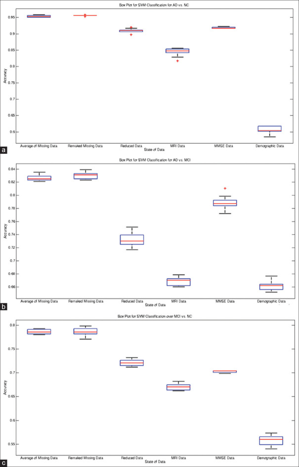
From Table 2 and Figures 5-8, the ROCs, boxplots, and AUC values increased after recovering missing data using autoencoder. Using the rebuilt missing data method, the boxplots compressed inward more than that of the averaging method for estimating the missing data. Such compression depicts higher stability in the classification model for rebuilt missing data method. Moreover, the accuracy of NC versus MCI classification with autoencoder increased after recovering missing data. Yet, exploiting the average of missing data obtained drastically better results in terms of distinguishing between MCI and AD patients. Line 6 of the table is bold that shows best accuracy and other performance measures in distinguishing MCI patients from NCs. As in Figure 8, after reducing the dimensionality of the input vector for classification, the Boxplots significantly compressed compared to that of the averaged missing data, which depicts less variance (i.e., higher stability) in the classification. Using PPV for missing data is more promising than other methods, and showed better prognosis capability with the proposed method.

Figure 5.

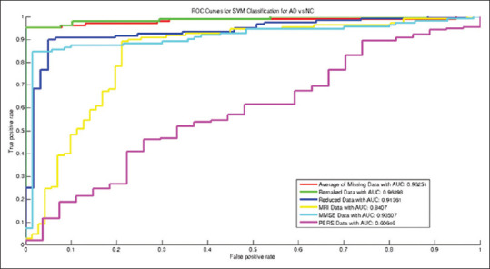
Receiver operating characteristic curves for Alzheimer's disease versus normal control classification

Figure 8.

Boxplots for recognition of AD, NC, and MCI subjects: (a) AD vs. NC. (b) AD vs. MCI. (c) MCI vs. NC

Figure 6.

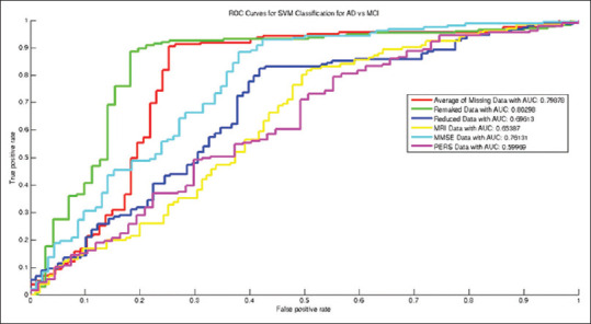
Receiver operating characteristic curves for mild cognitive impairment versus normal control classification

Discussion

Figures 5-7 and data in Table 2 show that the AUC values increased after recovering missing data (=0.964 for AD versus NC classification, and 0.803 and 0.799 values for AD versus MCI and for NC versus MCI classification, respectively). The boxplots after recovering missing data were clearly more compressed than that of the averaged missing data mode, which interprets more stability and reliability in the constructed classification model.

Figure 7.

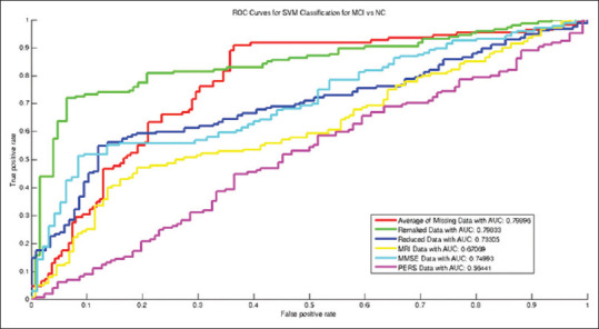
Receiver operating characteristic curves for Alzheimer's disease versus mild cognitive impairment classification

One important evidence is that utilizing the combination of different data sources can dramatically alleviate the weaknesses of each dataset. In this study, by combining five different data sources, we obtained high accuracy to distinguish AD and MCI patients and NCs from each other. The weakness can be the dependency of method on collecting several data sources and increasing missing data, a weakness that was handled well in this article using autoencoders.

In Table 3, the proposed method is compared to other methods. As shown in the table, proposed method outperformed other methods in most aspects of performance, and AUC of our method is above other methods. Due to normalization using natural logarithm and missing data imputation using autoencoder, rebuilt missing data method can estimate missed data more effectively. It also gained a higher performance in most aspects of AD diagnosis evaluation metrics. The true sensitivity rate using this method is 100%, which shows a perfect diagnosis of AD patients.

Table 3.

Comparison of the proposed method with other methods based on Alzheimer’s disease versus normal control classification

Method	Indicator, number of samples and data source	AD versus NC
		Accuracy (%)	Sensitivity (%)	Specificity (%)	AUC
Zhang et al., 2011[42]	MRI, PET, CSF, MMSE, ADAS-Cog (202, ADNI)	93.20	93.00	93.30	0.98
Dai et al., 2013[43]	MRI (83, OASIS)	90.81	92.59	90.33	0.94
Liu et al., 2016[44]	MRI, PET (710, ADNI)	94.65	95.03	91.76	0.95
da Silva Lopes et al., 2010[45]	EEG Signal (41,-)	71.5	82	61	-
Beheshti et al., 2017[27]	MRI (186, ADNI)	93.01	89.13	96.80	0.935
Mishra et al., 2018[46]	MRI (417, ADNI)	89.15	85.06	92.53	0.93
Khedher et al., 2015[47]	MRI (818, ADNI)	88.96	92.35	86.24	0.93
Lian et al., 2019[48]	MRI (1457, ADNI)	90.00	82.00	97.00	0.95
Ben Ahmed et al., 2014[49]	MRI (218, ADNI)	87.00	75.50	100	0.85
Zhou et al., 2018[50]	MRI (507, ADNI)	93.75	87.5	100	-
Suk et al., 2014[51]	MRI, PET, CSF, MMSE, ADAS-Cog (202, ADNI)	93.05	90.86	94.57	0.95
Maqsood et al., 2019[21]	MRI (392, OASIS)	89.66	100	82	-
Saravanakumar and Thangaraj 2019[52]	MRI (-, ADNI)	92.34	96	87.5	-
Proposed method (EL)	MRI, PET, CSF, MMSE (705, ADNI)	95.57	100	95.57	0.964

AD – Alzheimer’s disease; NC – Normal control; MRI – Magnetic resonance imaging; PET – Positron emission tomography; CSF – Cerebrospinal Fluid; MMSE – Mini-Mental State Examination; ADNI – Alzheimer’s Disease Neuroimaging Initiative; OASIS – Open Access Series of Imaging Studies; ADAS – Alzheimer’s Disease Assessment Scale

AUC = 1 means that the diagnostic test is perfect in the differentiation of diseased and nondiseased participants. This happens when the distribution of test results for the diseased and nondiseased participants has no overlap.[53] As can be seen, the AUC value in the proposed method is equal to 0.964 for the diagnosis of AD versus NC, which shows near excellent differentiation between diseased and nondiseased participants.

Conclusion

A novel method for distinguishing between AD and MCI patients and NCs was proposed. This has been done by missing data imputation and feature reduction using autoencoder, MR and PET images, MMSE scores, personal information, and CSF biomarkers using SVM with linear kernel. Data normalization was done using natural logarithm. The validity of the method was tested on the ADNI database. The accuracy of the method is tested using K-fold cross-validation (K = 10). To validate the effectiveness of proposed method, several tests are done on ADNI database, and it was compared with other AD diagnosis methods. The results on 705 baseline participants of ADNI show that the proposed method using multimodal data achieves a high accuracy for AD classification (accuracy = 95.57%) and also a significant improvement in area under the curve (AUC = 0.964). In addition, the boxplots are more compressed using rebuilt missing data by autoencoder. Using more modalities of data can help in improving classification metrics. In this article, an advanced method in machine learning, that is autoencoders, was used to overcome the limitation of small number of available individuals for training and testing classifier. It is useful in dealing with missing data for classification. The efficiency of this method was proved by the results of this article. In this article, only baseline data of the participants in ADNI database were used. As future work, longitudinal data can be used to predict the conversion from MCI to AD by finding the patterns of brain atrophy in multiple modalities, specifically in the ROI for AD in the MR and PET images.

Financial support and sponsorship

None.

Conflicts of interest

There are no conflicts of interest.

BIOGRAPHIES

Hamid Akramifard received the B.S. and his M.Sc. degree in the computer engineering (software) from PNU university, Iran in 2008 and 2012, respectively. He is now PhD Student in university of Tabriz, Iran. His research interests include image processing, medical image analysis, CAD systems for diagnosis brain disorders from 3D brain images. He has published papers in these domains.

Email: hamid.akramifard@tabrizu.ac.ir

Mohammad Ali Balafar was born in Tabriz, Iran, in June 1975. He received the Ph.D. degree in IT in 2010. Currently, he is an Assistant Professor. His research interests are in artificial intelligence and image and medical image processing. He has published several research papers in these areas.

Email: balafarila@tabrizu.ac.ir

Seyed Naser Razavi received the B.S. degree in computer engineering (software) in 2001 from Petroleum University of Technology and his M.Sc. and PhD degree in the computer engineering (Artificial Intelligence) from Iran University of Science and Technology in 2003 and 2010 respectively. His research of interests include artificial intelligence, multi-agent learning, and soft computing.

Email: n.razavi@tabrizu.ac.ir

Abd Rahman Ramli Born in 1940 Msia. He received the B.Sc., Electronics, at Universiti Kebangsaan Malaysia, Bangi, in 1982 and his M.Sc. Information Technology System, University of Strathclyde, U.K., 1985, and his PhD degree i Image Processing, University of Bradford, U.K, 1995. His research interests include Computer Engineering, Intelligent Systems, Robotics, Image processing, Multimedia System, Engineering. He has published many papers in these domains.

Email: arr302002@yahoo.com

References

- 1.Li S, Shi F, Pu F, Li X, Jiang T, Xie S, et al. Hippocampal shape analysis of Alzheimer disease based on machine learning methods. AJNR Am J Neuroradiol. 2007;28:1339–45. doi: 10.3174/ajnr.A0620. [DOI] [PMC free article] [PubMed] [Google Scholar]
- 2.Brookmeyer R, Johnson E, Ziegler-Graham K, Arrighi HM. Forecasting the global burden of Alzheimer's disease. Alzheimers Dement. 2007;3:186–91. doi: 10.1016/j.jalz.2007.04.381. [DOI] [PubMed] [Google Scholar]
- 3.Davatzikos C, Fan Y, Wu X, Shen D, Resnick SM. Detection of prodromal Alzheimer's disease via pattern classification of magnetic resonance imaging. Neurobiol Aging. 2008;29:514–23. doi: 10.1016/j.neurobiolaging.2006.11.010. [DOI] [PMC free article] [PubMed] [Google Scholar]
- 4.Klöppel S, Stonnington CM, Chu C, Draganski B, Scahill RI, Rohrer JD, et al. Automatic classification of MR scans in Alzheimer's disease. Brain. 2008;131:681–9. doi: 10.1093/brain/awm319. [DOI] [PMC free article] [PubMed] [Google Scholar]
- 5.Cuingnet R, Gerardin E, Tessieras J, Auzias G, Lehéricy S, Habert MO, et al. Automatic classification of patients with Alzheimer's disease from structural MRI: A comparison of ten methods using the ADNI database. Neuroimage. 2011;56:766–81. doi: 10.1016/j.neuroimage.2010.06.013. [DOI] [PubMed] [Google Scholar]
- 6.Foster NL, Heidebrink JL, Clark CM, Jagust WJ, Arnold SE, Barbas NR, et al. FDG-PET improves accuracy in distinguishing frontotemporal dementia and Alzheimer's disease. Brain. 2007;130:2616–35. doi: 10.1093/brain/awm177. [DOI] [PubMed] [Google Scholar]
- 7.Nordberg A, Rinne JO, Kadir A, Långström B. The use of PET in Alzheimer disease. Nat Rev Neurol. 2010;6:78–87. doi: 10.1038/nrneurol.2009.217. [DOI] [PubMed] [Google Scholar]
- 8.Dubois B, Feldman HH, Jacova C, DeKosky ST, Barberger-Gateau P, Cummings J, et al. Research criteria for the diagnosis of Alzheimer's disease: Revising the NINCDS-ADRDA criteria. Lancet Neurol. 2007;6:734–46. doi: 10.1016/S1474-4422(07)70178-3. [DOI] [PubMed] [Google Scholar]
- 9.Hajian-Tilaki K. Receiver operating characteristic (ROC) curve analysis for medical diagnostic test evaluation. Caspian J Intern Med. 2013;4:627–35. [PMC free article] [PubMed] [Google Scholar]
- 10.Acharya UR, Fernandes SL, WeiKoh JE, Ciaccio EJ, Fabell MK, Tanik UJ, et al. Automated detection of Alzheimer's disease using brain MRI images-A study with various feature extraction techniques. J Med Syst. 2019;43:302. doi: 10.1007/s10916-019-1428-9. [DOI] [PubMed] [Google Scholar]
- 11.Wang SH, Phillips P, Sui Y, Liu B, Yang M, Cheng H. Classification of Alzheimer's disease based on eight-layer convolutional neural network with leaky rectified linear unit and max pooling. J Med Syst. 2018;42:85. doi: 10.1007/s10916-018-0932-7. [DOI] [PubMed] [Google Scholar]
- 12.Duin RP. Classifiers in Almost Empty Spaces. Proceedings 15th International Conference on Pattern Recognition: IEEE. 2000:1–7. [Google Scholar]
- 13.Juottonen K, Laakso MP, Partanen K, Soininen H. Comparative MR analysis of the entorhinal cortex and hippocampus in diagnosing Alzheimer disease. AJNR Am J Neuroradiol. 1999;20:139–44. [PubMed] [Google Scholar]
- 14.Fox NC, Warrington EK, Freeborough PA, Hartikainen P, Kennedy AM, Stevens JM, et al. Presymptomatic hippocampal atrophy in Alzheimer's disease. A longitudinal MRI study. Brain. 1996;119(Pt 6):2001–7. doi: 10.1093/brain/119.6.2001. [DOI] [PubMed] [Google Scholar]
- 15.Killiany RJ, Moss MB, Albert MS, Sandor T, Tieman J, et al. Temporal lobe regions on magnetic resonance imaging identify patients with early Alzheimer's disease. Arch Neurol. 1993;50:949–54. doi: 10.1001/archneur.1993.00540090052010. [DOI] [PubMed] [Google Scholar]
- 16.Laakso MP, Soininen H, Partanen K, Lehtovirta M, Hallikainen M, Hänninen T, et al. MRI of the hippocampus in Alzheimer's disease: Sensitivity, specificity, and analysis of the incorrectly classified subjects. Neurobiol Aging. 1998;19:23–31. doi: 10.1016/s0197-4580(98)00006-2. [DOI] [PubMed] [Google Scholar]
- 17.Morra JH, Tu Z, Apostolova LG, Green AE, Avedissian C, Madsen SK, et al. Automated mapping of hippocampal atrophy in 1-year repeat MRI data from 490 subjects with Alzheimer's disease, mild cognitive impairment, and elderly controls. Neuroimage. 2009;45:S3–15. doi: 10.1016/j.neuroimage.2008.10.043. [DOI] [PMC free article] [PubMed] [Google Scholar]
- 18.Colliot O, Chételat G, Chupin M, Desgranges B, Magnin B, Benali H, et al. Discrimination between Alzheimer disease, mild cognitive impairment, and normal aging by using automated segmentation of the hippocampus. Radiology. 2008;248:194–201. doi: 10.1148/radiol.2481070876. [DOI] [PubMed] [Google Scholar]
- 19.Kantarci K. Magnetic resonance markers for early diagnosis and progression of Alzheimer's disease. Expert Rev Neurother. 2005;5:663–70. doi: 10.1586/14737175.5.5.663. [DOI] [PubMed] [Google Scholar]
- 20.Westman E, Simmons A, Zhang Y, Muehlboeck JS, Tunnard C, Liu Y, et al. Multivariate analysis of MRI data for Alzheimer's disease, mild cognitive impairment and healthy controls. Neuroimage. 2011;54:1178–87. doi: 10.1016/j.neuroimage.2010.08.044. [DOI] [PubMed] [Google Scholar]
- 21.Maqsood M, Nazir F, Khan U, Aadil F, Jamal H, Mehmood I, et al. Transfer learning assisted classification and detection of Alzheimer's disease stages using 3D MRI scans. Sensors (Basel) 2019;19:1–19. doi: 10.3390/s19112645. [DOI] [PMC free article] [PubMed] [Google Scholar]
- 22.Islam K, Damiati S, Sethi J, Suhail A, Pan G. Development of a label-free immunosensor for clusterin detection as an Alzheimer's biomarker. Sensors (Basel) 2018;18:1–12. doi: 10.3390/s18010308. [DOI] [PMC free article] [PubMed] [Google Scholar]
- 23.Toro CA, Gonzalo Martín C, García-Pedrero A, Menasalvas Ruiz E. Supervoxels-based histon as a new Alzheimer's disease imaging biomarker. Sensors (Basel) 2018;18:1–18. doi: 10.3390/s18061752. [DOI] [PMC free article] [PubMed] [Google Scholar]
- 24.Garyfallou GZ, Ketebu O, Sahin S, Mukaetova-Ladinska EB, Catt M, Yu EH. Electrochemical detection of plasma immunoglobulin as a biomarker for Alzheimer's disease. Sensors (Basel) 2017;17:1–13. doi: 10.3390/s17112464. [DOI] [PMC free article] [PubMed] [Google Scholar]
- 25.Lahmiri S. Image characterization by fractal descriptors in variational mode decomposition domain: Application to brain magnetic resonance. Physica A: Statist Mechan Appl. 2016;456:235–43. [Google Scholar]
- 26.Lahmiri S, Shmuel A. Performance of machine learning methods applied to structural MRI and ADAS cognitive scores in diagnosing Alzheimer's disease. Biomed Signal Proc Control. 2019;52:414–9. [Google Scholar]
- 27.Beheshti I, Demirel H, Matsuda H. Alzheimer's disease neuroimaging initiative.classification of Alzheimer's disease and prediction of mild cognitive impairment-to-Alzheimer's conversion from structural magnetic resource imaging using feature ranking and a genetic algorithm. Comput Biol Med. 2017;83:109–19. doi: 10.1016/j.compbiomed.2017.02.011. [DOI] [PubMed] [Google Scholar]
- 28.Spasov S, Passamonti L, Duggento A, Liò P, Toschi N. Alzheimer's disease neuroimaging initiative. A parameter-efficient deep learning approach to predict conversion from mild cognitive impairment to Alzheimer's disease. Neuroimage. 2019;189:276–87. doi: 10.1016/j.neuroimage.2019.01.031. [DOI] [PubMed] [Google Scholar]
- 29.Kashefpoor M, Rabbani H, Barekatain M. Automatic diagnosis of mild cognitive impairment using electroencephalogram spectral features. J Med Signals Sens. 2016;6:25–32. [PMC free article] [PubMed] [Google Scholar]
- 30.Catana C, Drzezga A, Heiss WD, Rosen BR. PET/MRI for neurologic applications. J Nucl Med. 2012;53:1916–25. doi: 10.2967/jnumed.112.105346. [DOI] [PMC free article] [PubMed] [Google Scholar]
- 31.Cheng B, Zhang D, Shen D. Domain transfer learning for MCI conversion prediction. Med Image Comput Comput Assist Interv. 2012;15:82–90. doi: 10.1007/978-3-642-33415-3_11. [DOI] [PMC free article] [PubMed] [Google Scholar]
- 32.Weiner MW, Veitch DP, Aisen PS, Beckett LA, Cairns NJ, Green RC, et al. The Alzheimer's disease neuroimaging initiative: A review of papers published since its inception. Alzheimer's and dementia J Alzheimer's Assoc. 2012;8(Suppl 1):S1–68. doi: 10.1016/j.jalz.2011.09.172. [DOI] [PMC free article] [PubMed] [Google Scholar]
- 33. [[Last accessed on 2020 Jan 14]]. Available from: https://medicine.uiowa.edu/mri/research/previousprojects .
- 34.Poultney C, Chopra S, Cun YL. Efficient learning of sparse representations with an energy-based model. In: Advances in Neural Information Processing Systems. Advances in. 2006:1137–44. [Google Scholar]
- 35.Ngiam J, Coates A, Lahiri A, Prochnow B, Ng A, Le QV. On Optimization Methods for Deep Learning. ICML-11. 2011:265–72. [Google Scholar]
- 36.Hinton GE. Connectionist learning procedures. Artific Intell. 1989;40:185–234. [Google Scholar]
- 37.Bengio Y, Lamblin P, Popovici D, Larochelle H. Greedy layer-wise training of deep networks. Adv Neural Inform Proc Syst. 2007;19:153. [Google Scholar]
- 38.Fan Y, Resnick SM, Wu X, Davatzikos C. Structural and functional biomarkers of prodromal Alzheimer's disease: A high-dimensional pattern classification study. Neuroimage. 2008;41:277–85. doi: 10.1016/j.neuroimage.2008.02.043. [DOI] [PMC free article] [PubMed] [Google Scholar]
- 39.Mourão-Miranda J, Bokde AL, Born C, Hampel H, Stetter M. Classifying brain states and determining the discriminating activation patterns: Support Vector Machine on functional MRI data. Neuroimage. 2005;28:980–95. doi: 10.1016/j.neuroimage.2005.06.070. [DOI] [PubMed] [Google Scholar]
- 40.Burges CJ. A tutorial on support vector machines for pattern recognition. Data Min Knowl Discov. 1998;2:121–67. [Google Scholar]
- 41.Shawe-Taylor J, Cristianini N. Learning Methods. UK: Cambridge University Press; 2000. Support vector machines and other kernel-Based. [Google Scholar]
- 42.Zhang D, Wang Y, Zhou L, Yuan H, Shen D. Alzheimer's disease neuroimaging initiative.Multimodal classification of Alzheimer's disease and mild cognitive impairment. Neuroimage. 2011;55:856–67. doi: 10.1016/j.neuroimage.2011.01.008. [DOI] [PMC free article] [PubMed] [Google Scholar]
- 43.Dai D, He H, Vogelstein JT, Hou Z. Accurate prediction of AD patients using cortical thickness networks. Mach Vis Appl. 2013;24:1445–57. [Google Scholar]
- 44.Liu J, Li M, Lan W, Wu FX, Pan Y, Wang J. Classification of Alzheimer's disease using whole brain hierarchical network. IEEE/ACM Trans Comput Biol Bioinform. 2018;15:624–32. doi: 10.1109/TCBB.2016.2635144. [DOI] [PubMed] [Google Scholar]
- 45.da Silva Lopes HF, Abe JM, Anghinah R. Application of paraconsistent artificial neural networks as a method of aid in the diagnosis of Alzheimer disease. J Med Syst. 2010;34:1073–81. doi: 10.1007/s10916-009-9325-2. [DOI] [PubMed] [Google Scholar]
- 46.Mishra S, Beheshti I, Khanna P. Initiative ftAsDN. A statistical region selection and randomized volumetric features selection framework for early detection of Alzheimer's disease. Int J Imag Syst Technol. 2018;28:302–14. [Google Scholar]
- 47.Khedher L, Ramírez J, Górriz JM, Brahim A, Segovia F. Early diagnosis of Alzheimer.s disease based on partial least squares, principal component analysis and support vector machine using segmented MRI images? Neurocomputing. 2015;151:139–50. [Google Scholar]
- 48.Lian C, Liu M, Zhang J, Shen D. Hierarchical fully convolutional network for joint atrophy localization and Alzheimer's disease diagnosis using structural MRI. IEEE Trans Pattern Anal Mach Intell. 2020;42:880–93. doi: 10.1109/TPAMI.2018.2889096. [DOI] [PMC free article] [PubMed] [Google Scholar]
- 49.Ben Ahmed O, Benois-Pineau J, Allard M, Ben Amar C, Catheline G. Classification of Alzheimer's disease subjects from MRI using hippocampal visual features. Multimedia Tools Appl. 2014;74:1249–66. [Google Scholar]
- 50.Zhou K, He W, Xu Y, Xiong G, Cai J. Feature selection and transfer learning for Alzheimer's disease clinical diagnosis. Appl Sci. 2018;8:1372. [Google Scholar]
- 51.Suk HI, Lee SW, Shen D. Alzheimer's disease neuroimaging initiative.Hierarchical feature representation and multimodal fusion with deep learning for AD/MCI diagnosis. Neuroimage. 2014;101:569–82. doi: 10.1016/j.neuroimage.2014.06.077. [DOI] [PMC free article] [PubMed] [Google Scholar]
- 52.Saravanakumar S, Thangaraj P. A computer aided diagnosis system for identifying Alzheimer's from MRI Scan using Improved Adaboost. J Med Syst. 2019;43:76. doi: 10.1007/s10916-018-1147-7. [DOI] [PubMed] [Google Scholar]
- 53.Folstein MF, Folstein SE, McHugh PR. “Mini-mental state”. A practical method for grading the cognitive state of patients for the clinician. J Psychiatr Res. 1975;12:189–98. doi: 10.1016/0022-3956(75)90026-6. [DOI] [PubMed] [Google Scholar]