Ordered Multinomial Regression for Genetic Association Analysis of Ordinal Phenotypes at Biobank Scale

Abstract

Logistic regression is the primary analysis tool for binary traits in genome-wide association studies (GWAS). Multinomial regression extends logistic regression to multiple categories. However, many phenotypes more naturally take ordered, discrete values. Examples include (1) subtypes defined from multiple sources of clinical information and (2) derived phenotypes generated by specific phenotyping algorithms for electronic health records (EHR). GWAS of ordinal traits have been problematic. Dichotomizing can lead to a range of arbitrary cutoff values, generating inconsistent, hard to interpret results. Using multinomial regression ignores trait value hierarchy and potentially loses power. Treating ordinal data as quantitative can lead to misleading inference. To address these issues, we analyze ordinal traits with an ordered, multinomial model. This approach increases power and leads to more interpretable results. We derive efficient algorithms for computing test statistics, making ordinal trait GWAS computationally practical for biobank scale data. Our method is available as a Julia package OrdinalGWAS.jl. Application to a COPDGene study confirms previously found signals based on binary case-control status, but with more significance. Additionally, we demonstrate the capability of our package to run on UK Biobank data by analyzing hypertension as an ordinal trait.

1. Introduction

Genome-wide association studies (GWAS) have enjoyed many successes and uncovered many clues to the genetic etiology of common diseases (Visscher et al., 2017). Large international consortia are now undertaking collaborative meta-analyses of the results of separate GWAS, utilizing effective sample sizes of tens of thousands of individuals for discovery and replication of increasingly modest genetic effects. Besides larger sample sizes, richer information is available. For instance, UK BioBank (Sudlow et al., 2015) and the Million Veteran Project (Gaziano et al., 2016, MVP) contain electronic health records (EHR) of individuals along with their genomic information. Big data bring both blessings and curses. One particular challenge is to properly define phenotypes that are both meaningful and powerful for genetic association testing. Both classical genetic epidemiology studies and EHR can possess hundreds of clinically relevant variables that are associated with the underlying phenotypes of interest. In contrast to directly available phenotypes, derived phenotypes are generated by potentially complicated phenotyping algorithms. Below are two examples.

COPD:

For classifying chronic obstructive pulmonary disease (COPD), the Global Initiative for Chronic Obstructive Lung Disease (GOLD) has proposed a simple algorithm to classify cases into stages 1 to 4, ranging from least severe to most severe (Vestbo et al., 2013). Three quantitative measures - forced expiratory volume (FEV1), forced vital capacity (FVC), and forced predicted expiratory volume (FEV1-predicted) are used to define the GOLD categories. Under this classification individuals with an FEV1/FVC ratio that is less than 0.70 are considered cases with severity increasing as FEV1-predicted value decreases. Individuals with an FEV1/FVC ratio that is at least 0.70 and an FEV1-predicted that is at least 80% are considered unaffected. Individuals with a FEV1/FVC ratio of at least 0.70, but have a low FEV1 predicted value (< 80%) are categorized into a GOLD unclassifiable category (Wan et al., 2011). These individuals are typically analyzed separately.

Not a case: FEV1/FVC ≥ 0.7 and FEV1-predicted ≥ 80%;

GOLD unclassifiable: FEV1/FVC ≥ 0.7 and FEV1-predicted < 80%;

GOLD stage 1 (mild): FEV1/FVC < 0.7 and FEV1-predicted ≥ 80%;

GOLD stage 2 (moderate): FEV1/FVC < 0.7 and 50% ≤ FEV1-predicted < 80%;

GOLD stage 3 (severe): FEV1/FVC < 0.7 and 30% ≤ FEV1-predicted < 50%;

GOLD stage 4 (very severe): FEV1/FVC < 0.7 and FEV1-predicted < 30%.

Figure 1 shows the correspondence between GOLD values and FEV1 predicted and FVC in the COPDGene study (Regan et al., 2010). One can carry out association testing of the bivariate trait (FEV1, FVC) or (FEV1/FVC, FVC). However multivariate modeling requires more parameters and the SNP effects may not correlate with GOLD stages, leading to hard to interpret results. Current GWAS were performed as a case-control study by treating individuals in the not a case category as controls and individuals with GOLD stages 2–4 as cases (Lutz et al., 2015). This approach, although statistically permissible, is inefficient because it assumes that the odds of disease are the same in groups 2–4 and omits group 1 entirely.

Figure 1:

GOLD stage values plotted with FVC and FEV1 predicted values.

EHR-based phenotyping:

Recently EHRs have emerged as a major data source for clinical and health services research. It has been a common practice to extract a patient’s disease status by automated phenotyping algorithms applied to EHR. Compared to the COPD example, the output from a phenotyping algorithm can have more categories as the underlying information is more complex. For example, Eastwood et al. (2016) developed an EHR algorithm to classify Type 2 diabetes (T2D) prevalence for the UK Biobank data, a biobank study that has phenotypic and genotypic data on over 500,000 people. Based on several different features in the EHR including diabetes diagnostic codes, diabetes medication, hyperglycemia in blood results defined by HbA_1c and fasting glucose levels, and presence of diabetes process of care codes, the algorithm categorizes individuals into different categories that relate to how likely they are to have diabetes. The algorithm classifies individuals into categories diabetes unlikely, possible type 2 diabetes, probable type 2 diabetes, and probable type 1 diabetes. Excluding those diagnosed with probable type 1 diabetes, ordinal phenotype labels are produced.

In both cases, the derived phenotypes take discrete, ordinal values. GOLD status clearly correlates with lung function. Labels from the EHR phenotyping algorithm for T2D indicate a hierarchy in the uncertainty in disease diagnosis. Often, the analysis strategy reduces ordinal values to two categories and resorts to logistic regression for case-control studies. COPDGene study reports GWAS results using not a case as controls and GOLD stages 2–4 as cases (Lutz et al., 2015). In the T2D phenotyping algorithm (Eastwood et al., 2016), there are 3 possible case groups. Similarly the algorithm for T2D control can also have multiple categories leading to at least three possible case-control cohorts. This freedom in the choice of case and control labels necessitates multiple analyses of the same data. Besides needing to pay a price for more testing, inconsistent findings from these correlated analyses can be difficult to reconcile. To address this issue, we propose using the ordered multinomial regression in association studies of ordinal traits. Taking ordinality into account can significantly boost the power in association studies.

Ordinal categorical data analysis has been a well studied area in statistics (Agresti, 2010). However it has attracted relatively less attention in genetic association studies. Morris et al. (2010) use multinomial regression for GWAS on multi-category traits. However,ignoring order information may lead decreased power. Several authors (O’Reilly et al., 2012; Wang, 2014) treat genotypes as ordinal responses and regress genotype dosage on multiple phenotypes. This retrospective approach ignores the ordinal feature of the phenotypes, is not easily generalized to multilocus models and gene-by-environmental interactions, and the results can be difficult to interpret. Treating the ordinal values as a univariate quantitative trait is also commonly used in practice. In the binary case, this strategy can be justified as a first order approximation to logistic regression (Agresti, 2018). For multiple categories, unequal distances between the categories can violate the assumptions of linear regression and lead to incorrect inference. For instance the distance between mild pain and moderate pain can be different from that between moderate pain and intense pain. However, the ordering is clear.

In this article we make several substantial contributions to GWAS for ordinal phenotypes. First, we systematically investigate the performance (type I error and power) of the ordered multinomial model in comparison with linear regression (treating ordinal traits as continuous traits), logistic regression (by dichotomizing ordinal traits), and multinomial regression (ignoring ordinality), in a variety of genetically plausible scenarios. Second, we derive an efficient testing strategy that is scalable to GWAS on biobank data. Our test applies to a single SNP, SNP-sets, or SNP-environment interactions. Third, we implement the methodology in the open source, high performance language Julia, which is available for free at https://github.com/OpenMendel/OrdinalGWAS.jl.

2. Methods

2.1. Association mapping with ordered multinomial models

We assume that trait Y takes ordinal values $j\in \{1,\dots ,J\}$. For example, in the COPD example J = 5 (excluding the unclassifiable category). Denote the cumulative probabilities of the trait value Y_i of i-th individual by

$${\alpha }_{ij}=\mathbb{P}\left(Y_i\le j\right).$$

Since α_iJ = 1, we only need to model J − 1 cumulative probabilities. Ordered multinomial model (Agresti, 2010) links α_ij to covariates x_i by

$$g\left({\alpha }_{ij}\right)={\theta }_j-x_i^T\beta ,j=1,\dots ,J-1,$$

where g is a strictly increasing link function, the intercepts ${\theta }_j$ satisfy the monotonicity constraint ${\theta }_1\le {\theta }_2\le \cdots \le {\theta }_{J-1}$, and β are the regression coefficients for covariates. This assumes regression coefficients β have the same effects on each of the the response categories but each category has its own intercept. The maximum likelihood estimate (MLE) of parameters $\theta =\left({\theta }_1,\dots ,{\theta }_{J-1}\right)$ and β is the maximizer of the sample loglikelihood. Different choices for the link function g lead to the classical proportional odds model (logit link), ordered Probit model (Probit link), or proportional hazards model (cloglog link). In practice, we choose the link function based on data according to goodness of fit measures such as the deviance (−2 × loglikelihood) at respective MLEs.

Under the logit link, the effect size can be interpreted as the expected change of the response variable in the ordered-log odds scale for a one unit increase in the predictor. For example, an effect size of 0.25 gives odds ratio of 1.28, which can be interpreted as the odds of being in a higher grouping (e.g. severe and most severe) is 1.28 times greater than being in a lower grouping (e.g. mild and moderate). Other link functions yield less interpretable effect sizes.

Suppose $x\in {ℝ}^p$ contains p non-genetic covariates, such as age, sex, smoking status and ethnic ancestry proxies (e.g. first few principal components of the genotype matrix), and $G\in {ℝ}^q$ contains the genetic information to be tested. For a single SNP, G is the scalar genotype dosage. For a SNP-set, G is the genotype dosage vector of q SNPs. To test gene-by-environment (G×E) including gene-by-drug interactions, G contains both genotype dosage and its interaction with other covariates. The likelihood ratio test (LRT) compares the loglikelihood at the MLE of the full model $g\left({\alpha }_{ij}\right)={\theta }_j-x^T\beta -G^T\gamma$ to that at the null model $g\left({\alpha }_{ij}\right)={\theta }_j-x^T\beta$. LRT enjoys higher power than the score test and Wald test at small to moderate sample sizes and also outputs effect sizes. However, in the GWAS setting, the full model needs to be re-fitted at each single SNP or SNP-set, which becomes computationally challenging for biobank scale data. In contrast, the score test only requires fitting the null model once for the entire GWAS. Testing each SNP only involves forming the score test statistic and is computationally cheap. A practical strategy is to perform a score test on all SNPs first and then only the top SNPs with the most significant score test p-values are reanalyzed by the slightly more powerful, but much slower, LRT. When sample size (e.g., n = 2500 or greater) is reasonable, score test provides comparable power with LRT (Supplementary Material Section S.6 and Supplementary Figure 9).

2.2. Score tests for individual SNPs, SNP-set or G×E

Let μ denote the inverse link function g⁻¹. The loglikelihood of a single observation $\left(y_i,x_i\right)$ is

$$\begin{gathered} {\ell }_i(\mathbf{\theta },\beta )=\ln \left({\alpha }_{ij}-{\alpha }_{i,j-1}\right) \\ =\ln \left[\mu \left({\theta }_{y_i}-x_i^T\beta \right)-\mu \left({\theta }_{y_i-1}-x_i^T\beta \right)\right] \\ =\ln p_{i{y}_i} \end{gathered}$$

with score (gradient)

$$\frac{\partial }{\partial {\theta }_j}{\ell }_i(\mathbf{\theta },\beta )=\{\begin{array}{l}{p}_{ij}^{-1}{\mu }^{\prime }\left({\theta }_j-x_i^T\beta \right)\\ -p_{i,j+1}^{-1}{\mu }^{\prime }\left({\theta }_j-x_i^T\beta \right)\\ 0\end{array}\begin{array}{l}{y}_i=j\\ y_i=j+1\\ \text{otherwise}\end{array}$$

$${\nabla }_{\beta }{\ell }_i(\mathbf{\theta },\beta )=-p_{i{y}_i}^{-1}\left[{\mu }^{\prime }\left({\theta }_{y_i}-x_i^T\beta \right)-{\mu }^{\prime }\left({\theta }_{y_i-1}-x_i^T\beta \right)\right]x_i$$

and Hessian

$$\frac{{\partial }^2}{\partial {\theta }_j\partial {\theta }_{j^{\prime }}}{\ell }_i(\mathbf{\theta },\beta )=\{\begin{array}{ll}{p}_{ij}^{-1}{\mu }^{″}\left({\theta }_j-x_i^T\beta \right)-{\left[p_{ij}^{-1}{\mu }^{\prime }\left({\theta }_j-x_i^T\beta \right)\right]}^2& y_i=j=j^{\prime }\\ -p_{i,j+1}^{-1}{\mu }^{″}\left({\theta }_j-x_i^T\beta \right)-{\left[p_{i,j+1}^{-1}{\mu }^{\prime }\left({\theta }_j-x_i^T\beta \right)\right]}^2& y_i=j+1=j^{\prime }+1\\ p_{ij}^{-2}{\mu }^{\prime }\left({\theta }_j-x_i^T\beta \right){\mu }^{\prime }\left({\theta }_{j-1}-x_i^T\beta \right)& y_i=j=j^{\prime }+1\\ p_{i,j+1}^{-2}{\mu }^{\prime }\left({\theta }_{j+1}-x_i^T\beta \right){\mu }^{\prime }\left({\theta }_j-x_i^T\beta \right)& y_i=j^{\prime }=j+1\\ 0& \text{otherwise}\end{array}$$

$${\nabla }_{\beta }\frac{\partial }{\partial {\theta }_j}{\ell }_i(\mathbf{\theta },\beta )=\{\begin{array}{ll}\left\{-p_{ij}^{-1}{\mu }^{″}\left({\theta }_j-x_i^T\beta \right)+p_{ij}^{-2}\left[{\mu }^{\prime }\left({\theta }_j-x_i^T\beta \right)-{\mu }^{\prime }\left({\theta }_{j-1}-x_i^T\beta \right)\right]{\mu }^{\prime }\left({\theta }_j-x_i^T\beta \right)\right\}{x}_i& y_i=j\\ \left\{p_{i,j+1}^{-1}{\mu }^{″}\left({\theta }_j-x_i^T\beta \right)-p_{i,j+1}^{-2}\left[{\mu }^{\prime }\left({\theta }_{j+1}-x_i^T\beta \right)-{\mu }^{\prime }\left({\theta }_j-x_i^T\beta \right)\right]{\mu }^{\prime }\left({\theta }_j-x_i^T\beta \right)\right\}{x}_i& y_i=j+1\\ 0& \text{otherwise}\end{array}$$

$${\nabla }_{\beta }^2{\ell }_i(\mathbf{\theta },\beta )=\left\{p_{i{y}_i}^{-1}\left[{\mu }^{″}\left({\theta }_{y_i}-x_i^T\beta \right)-{\mu }^{″}\left({\theta }_{y_i-1}-x_i^T\beta \right)\right]-p_{i{y}_i}^{-2}{\left[{\mu }^{\prime }\left({\theta }_{y_i}-x_i^T\beta \right)-{\mu }^{\prime }\left({\theta }_{y_i-1}-x_i^T\beta \right)\right]}^2\right\}{x}_i{x}_i^T.$$

The Fisher (expected) information matrix (FIM) has entries

$$\mathbb{E}\left[-\frac{{\partial }^2}{\partial {\theta }_j\partial {\theta }_{j^{\prime }}}{\ell }_i(\mathbf{\theta },\beta )\right]=\{\begin{array}{ll}\left(p_{ij}^{-1}+p_{i,j+1}^{-1}\right){\left[{\mu }^{\prime }\left({\theta }_j-x_i^T\beta \right)\right]}^2& j=j^{\prime }\\ -p_{ij}^{-1}{\mu }^{\prime }\left({\theta }_j-x_i^T\beta \right){\mu }^{\prime }\left({\theta }_{j-1}-x_i^T\beta \right)& j=j^{\prime }+1\\ -p_{i,j+1}^{-1}{\mu }^{\prime }\left({\theta }_j-x_i^T\beta \right){\mu }^{\prime }\left({\theta }_{j+1}-x_i^T\beta \right)& j^{\prime }=j+1\\ 0& \text{otherwise}\end{array}$$

$$\begin{gathered} \mathbb{E}\left[-{\nabla }_{\beta }\frac{\partial }{\partial {\theta }_j}{\ell }_i(\mathbf{\theta },\beta )\right]=[p_{ij}^{-1}{\mu }^{\prime }\left({\theta }_{j-1}-x_i^T\beta \right)-\left(p_{ij}^{-1}+p_{i,j+1}^{-1}\right){\mu }^{\prime }\left({\theta }_j-x_i^T\beta \right) \\ +p_{i,j+1}^{-1}{\mu }^{\prime }\left({\theta }_{j+1}-x_i^T\beta \right)]{\mu }^{\prime }\left({\theta }_j-x_i^T\beta \right)x_i \end{gathered}$$

$$\mathbb{E}\left[-{\nabla }_{\beta }^2{\ell }_i(\mathbf{\theta },\beta )\right]=\sum _{j=1}^J{p}_{ij}^{-1}{\left[{\mu }^{\prime }\left({\theta }_j-x_i^T\beta \right)-{\mu }^{\prime }\left({\theta }_{j-1}-x_i^T\beta \right)\right]}^2{x}_i{x}_i^T.$$

We partition the FIM at the null model, i.e., ${\gamma }_1=\cdots ={\gamma }_q=0$, as

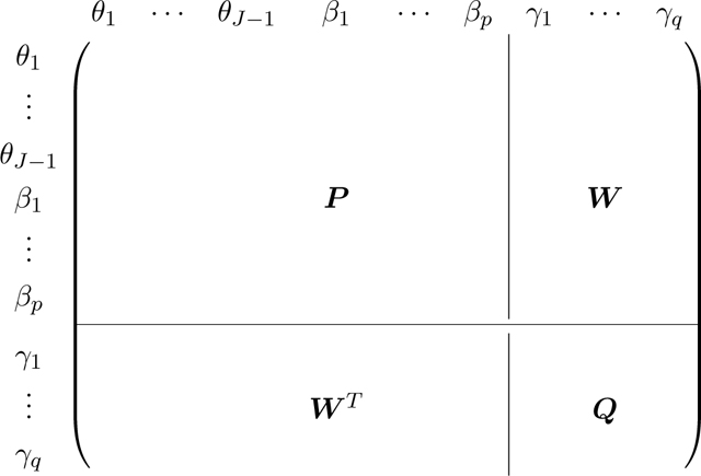and denote the score vector (gradient) with respect to γ at null model as R. To test significance of γ, we calculate the score test statistic as

$$S={\mathit{R}}^T{\left(\mathit{Q}-{\mathit{W}}^T{\mathit{P}}^{-1}\mathit{W}\right)}^{-1}\mathit{R}$$

and compare to the Chi-square distribution with q degrees of freedom. P⁻¹ is pre-computed and, for each SNP or SNP set, we only need to update W and Q, which cost O(q³ + nq²) flops. Since q is typically small, the computation cost scales linearly with sample size, making it scalable to biobank data with 10⁵ ∼ 10⁶ samples and millions of SNPs.

2.3. Software

We have developed a package using the high performance dynamic programming language Julia (Bezanson, Edelman, Karpinski, & Shah, 2017) to perform GWAS analyses on single SNPs, SNP sets, or G×E interactions (https://github.com/OpenMendel/OrdinalGWAS.jl) as part of the OpenMendel umbrella (Zhou et al. (2019)). Users can run the software on Julia version 1.0 or later, or use Docker without installing Julia. Our package allows easy specification of the type of test (score or LRT), link function, covariates to include in null model, masks for SNPs or samples, and formula for interactions. The package requires a covariate file, genotype data, and a formula for the null model. It outputs a text file in comma separated values (CSV) format with p-values and relevant information for each SNP, including fitted effect size coefficients if the LRT option is specified, and another text file with the fitted null-model.

For large data sets, a practical strategy is to perform score tests first, then re-do an LRT for the most promising SNPs according to score test p-values. Running the score test allows very quick screening of significant SNPs compared to the LRT, which is especially advantageous for large datasets. As mentioned in the methods section, the two tests are asymptotically equivalent and when tested through simulations, the two tests yielded similar power even at a modest sample size of 2500. It is recommended to screen SNPs using the score test if time and computational resources are limited, and then evaluate the LRT on SNPs that meet a threshold significant to the investigator to retrieve the LRT p-value along with the estimated effect size. If the investigator needs effect size estimates of all SNPs or if computational resources and time are not important, then using the LRT for all SNPs will be preferable. The choice of link function may depend on several factors. The logit link function yields easily interpretable results and is widely used as it results in the proportional odds model, but the results can change based on the link function used. In our analyses, we use the link function that yields the highest loglikelihood for the null model.

3. Results

3.1. Simulated data examples

To assess the adequacy of the ordered multinomial model in a GWAS setting, we performed type I error and power comparisons between ordered multinomial regression with logit link function, linear regression, logistic regression, and multinomial regression in a simulation setting. We generated covariates age and gender from Normal(μ = 45, σ² = 64) and Bernoulli(p_male = 0.51) distributions respectively. The effects of the gender and standardized age variables were set to 1.0 and 2.0 respectively. The genotype vector was generated according to Hardy-Weinberg Equilibrium (HWE) with varying minor allele frequencies (MAFs) between 5% and 20%. The response variable was generated using a proportional odds assumption from the simulated covariates, genotype vector, and effect sizes with a total of 4 ordered categories. For the logistic regression, we dichotomized the ordered response variable as y_logit = 0 if the ordinal variable was 1 or 2, and y_logit = 1 if the ordinal variable was 3 or 4.

The heterozygous ordered log odds multiplicative effect size for each minor allele of the genotype vector, γ, was varied from the null value of 0 to 0.5. Different intercept values, θ, were also tested. We used 10⁶ replicates for each null effect size scenario to evaluate the type I error. We used 1000 replicates at each non-zero effect size to test the power of the model. Sample size varied from 2000 to 10, 000. The p-values of the ordered multinomial regression are derived from using the score test statistic. Results of different settings for type I error are shown in Table 2. QQ plots where θ = (0.1, 3.0, 3.1), the MAF = 0.2, and the sample size was 5, 000 are displayed in Figure 2. The p-values for the logistic and multinomial regression show heavy tails, indicating overall significant (inflated) p-values.

Table 2:

Empirical type I error rates (×10⁻⁵) at significance level 10⁻⁵ based on 1,000,000 replicates. All Standard errors for all estimated type I errors are all smaller than 4.25×10⁻⁶.

		θ = (1.0; 1.2; 1.4)				θ = (0.1; 3.0; 3.1)
n	MAF	Linear	Logistic	Multinomial	Ordinal	Linear	Logistic	Multinomial	Ordinal
2000	0.05	1.2	1.0	1.2	1.0	1.0	0.8	0.5	1.0
	0.10	1.6	1.3	0.9	1.1	0.8	0.6	0.5	0.9
	0.20	0.7	0.7	1.0	0.8	1.8	0.5	0.6	1.4
5000	0.05	0.8	0.6	1.5	0.5	1.4	0.5	0.6	1.3
	0.10	0.9	0.7	0.9	0.8	0.9	1.5	0.9	0.4
	0.20	1.0	0.9	1.2	0.8	0.6	1.0	0.5	1.2
10000	0.05	0.6	0.3	1.0	0.4	1.5	1.4	1.7	1.4
	0.10	1.3	0.6	1.0	0.8	1.0	1.1	0.8	1.1
	0.20	0.8	0.9	1.3	0.9	1.3	1.1	1.0	0.6

Figure 2:

QQ plots of p-values from type I error simulation for θ = (0.1, 3.0, 3.1) at MAF = 0.2 and sample size n = 5000. Regression type is displayed above each plot.

The results of our power analysis are displayed in Figure 3 where a significance level of 10⁻⁵ was used. We show that there are conditions where the ordered multinomial model has distinctively higher power than other commonly used existing methods. When the underlying intercept values, θ, are disproportionately non-uniform (right panel of 3), which can happen in a real-world setting, using logistic regression can have over 30% reduced power over the ordered multinomial regression. When θ is set to a more favorable scenario for logistic regression, there is less of a difference in power, but the ordered multinomial method still performs well, where the multinomial regression does less favorably.

Figure 3:

These plots display the power of ordered multinomial, linear regression, logistic regression, and multinomial regression based on 1000 replicates of generating data with four ordered categories from a proportional odds assumption with a sample size of n = 5000 at a 10⁻⁵ significance level. Minor allele frequency of the simulated causal variant is 0.20 and intercept values for the simulated response variable are θ = (1.0, 1.2, 1.4) for the plot on the left and θ = (0.1, 3.0, 3.1) for the plot on the right. Effect sizes, γ, range from 0.0 to 0.5.

In terms of power, the ordered multinomial method has several advantages. It does not assume linear spacing between ordinal categories, so it applies to real-world settings where the definition of ordered variables depends on several different measures. The ordered multinomial model also only needs to estimate one more parameter for each category added (K − 2 more parameters than binary logistic regression for K ordinal categories). In contrast the multinomial regression requires an additional set of all parameters for each additional category, which can result in overfitting and a loss in power. The use of logistic regression in ordinal data has been ad hoc. It is common to run several regressions on different grouping of cases and controls and then examine the overlap. Another approach is to omit the in-between categories, which reduces sample size and power. Using an ordered multinomial regression allows for much of the data to be used while maintaining a rather parsimonious model.

We detail power simulation results for G×E and SNP-set analysis in supplementary material S.5. In summary, our results are similar to the single SNP results in that there are highly plausible scenarios in which the ordinal multinomial model outperforms the common existing methods for both G×E and SNP-set analyses.

3.2. COPDGene GWAS

We apply our method to COPDGene, a large case-control sample of well-characterized smokers from a genome-wide association study of respiratory disease. Data were requested through NCBI’s dbGAP repository under study accession: phs000179.v6.p2. It includes 10,192 non-hispanic white (NHW) and African American (AA) current and former smokers with airflow obstruction ranging from none to GOLD stage 4 (very severe) COPD. The study design of COPDGene has been reported previously (Regan et al., 2010). Briefly, the subjects are included between the ages of 45 and 80 with at least a 10 pack-year smoking history. Exclusion criteria include pregnancy, history of other lung disease except asthma, prior lobectomy or lung volume reduction surgery, active cancer undergoing treatment, or known or suspected lung cancer. Because Lutz et al. (2015) analyzed AA and NHW separately, we applied our method to the larger of the two populations, the NHW population, which includes 6678 individuals after data quality control and exclusions. Details concerning genotyping, quality control, and imputation are posted on the COPDGene website (http://www.copdgene.org). Variable final gold based on the GOLD’s guidelines for classifying COPD was used. Summary statistics of the cohort are shown in Supplementary Material section S.1 and Supplementary Table 1. Histograms of minor allele frequencies, missing SNPs per person, and missing people per SNP of the NHW COPDGene genotype data are shown in Supplementary Material Figure 1.

We compare our method using the logit link function to the method previously used to analyze the data, logistic regression, and find that our ordinal regression method produces similar, and in some cases more significant results. After excluding data from the individuals with missing data (19 individuals), and those in the unclassifiable category (FEV1/FVC ratio ≥ 0.7 but predicted FEV1 ≤ 80%) (698 individuals), ordinal multinomial GWAS was run on data from a total of 5,953 individuals and 630,860 SNPs controlling for gender, age, pack years, height, and the first ten principal components as was done in Lutz et al. (2015). For logistic regression, we ran the model using category 0 as controls and categories 2–4 as cases. The score test was used on all SNPs, with the LRT run for the top hits (p-value < 10⁻⁶). Figure 4 presents the Manhattan plots of the results of the logistic and ordered multinomial GWAS. The ordered multinomial and logistic regressions produce similar results with peaks appearing on chromosome 15 (p-value = 2.761 × 10⁻¹¹ for ordered multinomial and p-value = 1.232 × 10⁻⁸ for logistic). The difference in the magnitude of the p-values is quite impressive, with the more significant signal coming from the ordered multinomial regression. Ordered multinomial regression produces potential signals on chromosomes 3 and 4, whereas logistic regression produces a signal on chromosome 4 and but no clear sign of a potential signal on chromosome 3. The nearest gene to the SNP relating to the potential signal using ordered multinomial regression (p-value = 5.731 × 10⁻⁷) on chromosome 3 is EEFSEC, which has been shown to be associated with COPD (Hobbs et al., 2017). Locuszoom plot of association results, linkage disequilibrium and recombination rates around the top hits can be found in Supplementary Material section S.2 and Supplementary Figure 2.

Figure 4:

Manhattan plots for the COPD GWAS results in COPDGene. Left is the Manhattan plot using logistic regression. Right is the Manhattan plot using ordered multinomial regression. The blue line indicates the Bonferroni correction threshold.

Our implementation in OrdinalGWAS.jl is fast. GWAS analysis on a standard laptop running Mac OS with a quad-core processor took just under 3.5 minutes.

Under an extreme case, where we remove all individuals in the middle and only run the GWAS on individuals falling under not a case and GOLD stage 4, we see a general trend that effect sizes are larger, but p-values are less significant. Manhattan plot for this analysis is in Supplementary Figure 3. Here we see that using different criteria for binary variables can lead to different, and therefore less interpretable results. Since the cutoff point for generation of binary variables from ordinal ones is arbitrary, two analyses on the same data may yield different results. Although linear regression on ordinal variables leads to problems with interpretability, we ran linear regression GWAS on the COPDGene data and have included the Manhattan plot in Supplementary Figure 4. Interestingly, but not completely unexpected when dealing with real data, the peak on chromosome 15 is slightly more significant with linear regression than with ordinal multinomial regression.

3.3. Hypertension GWAS in UK Biobank

Hypertension is a heritable trait (Muñoz et al., 2016) and a modifiable driver of risk for stroke and coronary artery disease. It is a leading cause of global mortality and morbidity (GBD 2015 Risk Factors Collaborators, 2016). GWAS meta-analyses and analyses of custom or exome content have identified and replicated genetic variants associated with elevated blood pressure (BP) and severe hypertension at over 120 loci (Warren et al., 2017). These researchers carefully construct a single quantitative measure of blood pressure and find many associated loci, replicating previous findings and discovering new potential loci. However none of the existing studies look at SNPs associated with hypertension as an ordinal trait due to the lack of computational tools for analyzing ordinal outcomes at biobank scale. Here we demonstrate the ability of our software by applying it to the UK Biobank blood pressure dataset. The UK Biobank is a prospective cohort study of approximately 500,000 men and women aged 40 to 69 years with extensive baseline phenotypic measurements, stored biological samples and follow-up by EHR linkage (Sudlow et al., 2015). In this section, we report the association between five categories of hypertension (defined using 2017 guidelines (Whelton et al., 2018)) and genetic variants among participants in UK Biobank.

We define hypertensive phenotype based on 2017 Guideline for the Prevention, Detection, Evaluation, and Management of High Blood Pressure in Adults (Whelton et al., 2018).

Normal: SBP/DBP less than 120/80 mm Hg;

Elevated: SBP between 120–129 mm Hg and DBP less than 80 mm Hg;

Stage 1: SBP between 130–139 mm Hg or DBP between 80–89 mm Hg;

Stage 2: SBP at least 140 mm Hg or DBP at least 90 mm Hg;)

Hypertensive crisis: SBP over 180 mm Hg and/or DBP over 120 mm Hg.

Our GWAS analysis is performed using data from the second release of UK Biobank participants. Individuals from UK Biobank were genotyped at ~800,000 SNPs with a custom Affymetrix UK Biobank Axiom array. Non-imputed data were used in the analysis. Information on UK Biobank array design and protocols is available on the UK Biobank website. Following quality control procedures already carried out centrally by UK Biobank, we excluded samples with quality control failures, sex discordance and high heterozygosity/missingness (n=968). We further restricted our data to a subset of individuals of European ancestry and exclude first- and second-degree relatives using kinship data leading to the exclusion of data from another 150,832 individuals. This leads to a sample of n = 337,545 individuals. We filtered samples by 98% genotyping success rate on all chromosomes and SNPs by 99% genotyping success rate and a MAF of at least 2% over the whole population. These measures result in n = 185,565 individuals and 464,137 SNPs for analysis.

Baseline characteristic of 185,565 participants are shown in Supplementary Material section S.3 and Supplementary Table 2. There are 34,009 (10.0%) participants who had undertaken hypertension related medications at baseline. These people were excluded from the analysis. Five categories of hypertension were first defined by their systolic and diastolic blood pressure (SBP and DBP). The final set of individuals are distributed as 16% with normal blood pressure, 13% with elevated blood pressure, 27% in stage 1 hypertension, 40% in stage 2 hypertension, and 2% in hypertension crisis. We compare our method to GWAS using logistic regression, defining hypertension cases as belonging to stage 2 or higher as done in Warren et al. (2017). We recalculated principal components using FlashPCA after filtering individuals and SNPs through QC filters, because the subset of individuals we analyze are exclusively of British ancestry, and the original principal components were calculated before filtering (Abraham, Qiu, & Inouye, 2017). Our hypertension GWAS analysis includes the following covariates: sex, center, age, age², BMI, and the top ten principal components to adjust for ancestry/relatedness. We used the logit link function for the ordered multinomial GWAS as it yielded the highest loglikelihood for the null model. The score test was used on all SNPs, with the LRT run for the top hits (p-value < 10⁻⁸). The Manhattan plots are displayed in Figure 5 and the QQ plots in Supplementary Figure 5. Information on the top hits from OrdinalGWAS on the UK Biobank data is included in the Supplementary Tables. The genomic inflation factor from OrdinalGWAS is 1.252, a high, but expected value for polygenic traits like blood pressure in a GWAS that includes a large sample size and many SNPs in high LD (Evangelou et al., 2018). The analysis took 181 minutes to run on a standard laptop with a quad-core processor running on Mac OS.

Figure 5:

Manhattan plots for the hypertension GWAS results in UK Biobank. Left is the Manhattan plot using logistic regression. Right is the Manhattan plot using ordered multinomial regression. The blue line indicates the Bonferroni correction threshold.

The use of logistic regression on the binary hypertension variable yielded hits at similar locations, with less significance. The genomic inflation factor was similarly high at 1.173. As in the case of our COPD analysis, the logistic and ordinal multinomial regression analyses gave qualitatively similar results with, in general, the ordinal multinomial regression providing more power than the ordinal regression. Overall our results are consistent with the polygenic nature of blood pressure with log odds ratios of significant hits ranging between −0.0773 and 0.1107. In general, rare variants tended to have higher effect sizes than common variants.

We also performed SNP-set and G×E analysis to demonstrate our software’s capability to do so on the UK Biobank data. G×E was run with sex as the environmental variable on the SNPs that passed (p-value < 10⁻⁸) from the original analysis. Results of this analysis are found in Supplementary Table 4. The Manhattan plot for the SNP-set analysis with a window size of 20 SNPs is in Supplementary Figure 6.

4. Discussion

We have developed a method tailored to GWAS on ordinal traits. In many instances, it increases power and allows for a more simplified setup and interpretation than existing approaches, since cutpoints for transforming ordinal traits into binary traits are usually arbitrary and not agreed upon. The strategy of conducting a score test on each SNP and then only running a likelihood ratio test on the top SNPs allows our method to scale to biobank scale GWAS data sets.

We have shown that the model has appropriate type I error when looking at various sample sizes and minor allele frequencies, while logistic and multinomial regression can result in inflated type I error under certain conditions. We have shown situations where using ordered multinomial regression can lead to significant power gains over logistic regression when the specification of the logistic case/control response variable is poor. Our framework will be most useful in finding causal loci related to complex diseases that have no clear distinction between what constitutes a case versus a control, but where disease progression can be well specified.

Besides single-SNP GWAS, our software also implements GWAS for SNP sets and G×E interactions. This allows for many more types of GWAS to be performed with ordinal outcomes and covers much of the current existing needs.

Other models that relax the proportional odds assumption may be useful to explore. These models, such as a partial proportional odds model (Peterson & Harrell, 1990), allow for some covariates to violate the proportional odds assumption, but they lead to less parsimonious models and less interpretable results since a separate effect size and p-value is produced for each group of ordered outcomes.

For the COPDGene data, our method had a much stronger signal than logistic regression on chromosome 15. Ordered multinomial regression had a suggestive signal on chromosome 3 that has been associated with COPD from another study, but missed by the logistic regression. Although we did not recover the Bonferroni-corrected signal that logistic regression did in the COPDGene data, the signal on the SNP was still suggestive and the lowest p-value above the threshold. We suspect the lower p-value could be due to the fact that the SNP heavily violated the proportional odds assumption. However, it is difficult to verify this. Current tests for the proportional odds assumption have been described as very liberal, often leading to rejection when there are many parameters in the model or the sample size is large (Allison, 1999).

Our software scales to biobank data with hundreds of thousands of individuals genotyped at hundreds of thousands of SNPs. Our goal in analyzing the UK Biobank blood pressure data were not to report new findings for hypertension, but to demonstrate the scalability of our method and to show how the results of ordinal multinomial regression differ from those of a standard logistic regression analysis. When applied to the UK Biobank data, signals were generally substantially stronger than those from logistic regression on the binary hypertension variable using the same individuals in both analyses. Comparison to other analyses of the UK Biobank blood pressure data is not straightforward and we do not recommend it. There are a number ways of our treatment of the data deviates from previous studies besides treating the outcomes as ordered categories (Evangelou et al., 2018; Warren et al., 2017). We used non-imputed, hard genotype calls whereas other studies used imputed fractional dosage data. By not using imputation we analyzed far fewer markers and excluded more individuals. We used genotype and phenotype data on 185,565 individuals of British ancestry, whereas other studies used genotype and phenotype data on individuals with European ancestry. We excluded individuals who took blood pressure medications whereas other studies adjusted for medication use. Our results use only UK Biobank data whereas other studies report results of meta-analyses. It is thus not surprising that our results differ from previous blood pressure trait GWAS with UK Biobank. Still, even with all the caveats, a large number of the loci, notably CACNB2, MTHFR, and PLCD3, have been reported to be linked to hypertension in previous studies (Levy et al., 2009; Newton-Cheh et al., 2009; Thomsen et al., 2017).

In summary, we have developed an ordinal multinomial regression approach for GWAS of hundreds of thousands of individuals. The method has similar computational requirements as score tests for logistic regression but it is more powerful for analyzing ordinal data. Our software is easy to use and freely available at https://github.com/OpenMendel/OrdinalGWAS.jl as part of the OpenMendel ecosystem (Lange et al., 2013; Zhou et al., 2019).

Table 1:

Commonly used ordered multinomial models.

Link	g	Model
Logit	$g(\alpha )=\alpha /(1-\alpha )$	proportional odds model
Probit	$g(\alpha )={\mathbf{\text{Φ}}}^{-1}(\alpha )$	ordred Probit model
Cloglog	$g(\alpha )=\log (-\log (1-\alpha ))$	proportional hazard model

References

- Abraham G, Qiu Y, & Inouye M. (2017). FlashPCA2: principal component analysis of Biobank-scale genotype datasets. Bioinformatics, 33, 2776–2778. doi: 10.1093/bioinformatics/btx299 [DOI] [PubMed] [Google Scholar]
- Agresti A. (2010). Analysis of ordinal categorical data (Second ed.). John Wiley & Sons, Inc., Hoboken, NJ. doi: 10.1002/9780470594001 [DOI] [Google Scholar]
- Agresti A. (2018). An introduction to categorical data analysis. Wiley. [Google Scholar]
- Allison PD (1999). Logistic regression using the SAS system: Theory and application. SAS Institute Corp., USA. [Google Scholar]
- Bezanson J, Edelman A, Karpinski S, & Shah VB (2017). Julia: A fresh approach to numerical computing. SIAM Review, 59, 65–98. doi: 10.1137/141000671 [DOI] [Google Scholar]
- Eastwood SV, Mathur R, Atkinson M, Brophy S, Sudlow C, Flaig R, … Chaturvedi N. (2016). Algorithms for the capture and adjudication of prevalent and incident diabetes in uk biobank. PLOS ONE, 11, 1–18. doi: 10.1371/journal.pone.0162388 [DOI] [PMC free article] [PubMed] [Google Scholar]
- Evangelou E, Warren HR, Mosen-Ansorena D, Mifsud B, Pazoki R, Gao H, … Million Veteran Program (2018). Genetic analysis of over 1 million people identifies 535 new loci associated with blood pressure traits. Nature genetics, 50, 1412–1425. doi: 10.1038/s41588-018-0205-x [DOI] [PMC free article] [PubMed] [Google Scholar]
- Gaziano JM, Concato J, Brophy M, Fiore L, Pyarajan S, Breeling J, … O’Leary TJ (2016). Million Veteran Program: A mega-biobank to study genetic influences on health and disease. Journal of Clinical Epidemiology, 70, 214–223. doi: 10.1016/j.jclinepi.2015.09.016 [DOI] [PubMed] [Google Scholar]
- GBD 2015 Risk Factors Collaborators. (2016). Global, regional, and national comparative risk assessment of 79 behavioural, environmental and occupational, and metabolic risks or clusters of risks, 1990–2015: a systematic analysis for the global burden of disease study 2015. Lancet (London, England), 388, 1659–1724. doi: 10.1016/S0140-6736(16)31679-8 [DOI] [PMC free article] [PubMed] [Google Scholar]
- Hobbs BD, de Jong K, Lamontagne M, Bossé Y, Shrine N, Artigas MS, … International COPD Genetics Consortium (2017). Genetic loci associated with chronic obstructive pulmonary disease overlap with loci for lung function and pulmonary fibrosis. Nature Genetics, 49, 426 EP −. doi: 10.1038/ng.3752 [DOI] [PMC free article] [PubMed] [Google Scholar]
- Lange K, Papp J, Sinsheimer J, Sripracha R, Zhou H, & Sobel E. (2013). Mendel: the Swiss army knife of genetic analysis programs. Bioinformatics, 29, 1568–1570. [DOI] [PMC free article] [PubMed] [Google Scholar]
- Levy D, Ehret GB, Rice K, Verwoert GC, Launer LJ, Dehghan A, … van Duijn CM (2009). Genome-wide association study of blood pressure and hypertension. Nature genetics, 41, 677–687. doi: 10.1038/ng.384 [DOI] [PMC free article] [PubMed] [Google Scholar]
- Lutz SM, Cho MH, Young K, Hersh CP, Castaldi PJ, McDonald M-L, … ECLIPSE Investigators, and COPDGene Investigators (2015). A genome-wide association study identifies risk loci for spirometric measures among smokers of european and african ancestry. BMC Genetics, 16, 138. doi: 10.1186/s12863-015-0299-4 [DOI] [PMC free article] [PubMed] [Google Scholar]
- Morris AP, Lindgren CM, Zeggini E, Timpson NJ, Frayling TM, Hattersley AT, & McCarthy MI (2010). A powerful approach to sub-phenotype analysis in population-based genetic association studies. Genetic Epidemiology, 34, 335–343. doi: 10.1002/gepi.20486 [DOI] [PMC free article] [PubMed] [Google Scholar]
- Muñoz M, Pong-Wong R, Canela-Xandri O, Rawlik K, Haley CS, & Tenesa A. (2016). Evaluating the contribution of genetics and familial shared environment to common disease using the UK Biobank. Nature Genetics, 48, 980. doi: 10.1038/ng.3618 [DOI] [PMC free article] [PubMed] [Google Scholar]
- Newton-Cheh C, Johnson T, Gateva V, Tobin MD, Bochud M, Coin L, … Munroe PB (2009). Genome-wide association study identifies eight loci associated with blood pressure. Nature genetics, 41, 666–676. doi: 10.1038/ng.361 [DOI] [PMC free article] [PubMed] [Google Scholar]
- O’Reilly PF, Hoggart CJ, Pomyen Y, Calboli FCF, Elliott P, Jarvelin M-R, & Coin LJM (2012). MultiPhen: joint model of multiple phenotypes can increase discovery in GWAS. PLoS ONE, 7, 1–1. doi: 10.1371/journal.pone.0034861 [DOI] [PMC free article] [PubMed] [Google Scholar]
- Peterson B, & Harrell FE (1990). Partial proportional odds models for ordinal response variables. Journal of the Royal Statistical Society. Series C (Applied Statistics), 39, 205–217. doi: 10.2307/2347760 [DOI] [Google Scholar]
- Regan EA, Hokanson JE, Murphy JR, Make B, Lynch DA, Beaty TH, … Crapo JD (2010). Genetic epidemiology of COPD (COPDGene) study design. COPD: Journal of Chronic Obstructive Pulmonary Disease, 7, 32–43. doi: 10.3109/15412550903499522 [DOI] [PMC free article] [PubMed] [Google Scholar]
- Sudlow C, Gallacher J, Allen N, Beral V, Burton P, Danesh J, … Collins R. (2015). Uk biobank: an open access resource for identifying the causes of a wide range of complex diseases of middle and old age. PLoS medicine, 12, e1001779–e1001779. doi: 10.1371/journal.pmed.1001779 [DOI] [PMC free article] [PubMed] [Google Scholar]
- Thomsen LCV, McCarthy NS, Melton PE, Cadby G, Austgulen R, Nygård OK, … Iversen A-C (2017). The antihypertensive mthfr gene polymorphism rs17367504-g is a possible novel protective locus for preeclampsia. Journal of hypertension, 35, 132–139. doi: 10.1097/HJH.0000000000001131 [DOI] [PMC free article] [PubMed] [Google Scholar]
- Vestbo J, Hurd SS, Agust AG, Jones PW, Vogelmeier C, Anzueto A, … Rodriguez-Roisin R. (2013). Global strategy for the diagnosis, management, and prevention of chronic obstructive pulmonary disease. American Journal of Respiratory and Critical Care Medicine, 187, 347–365. (PMID: 22878278) doi: 10.1164/rccm.201204-0596PP [DOI] [PubMed] [Google Scholar]
- Visscher PM, Wray NR, Zhang Q, Sklar P, McCarthy MI, Brown MA, & Yang J. (2017). 10 years of GWAS discovery: biology, function, and translation. The American Journal of Human Genetics, 101, 5–22. doi: 10.1016/j.ajhg.2017.06.005 [DOI] [PMC free article] [PubMed] [Google Scholar]
- Wan ES, Hokanson JE, Murphy JR, Regan EA, Make BJ, Lynch DA, … COPDGene Investigators (2011). Clinical and radiographic predictors of gold–unclassified smokers in the copdgene study. American journal of respiratory and critical care medicine, 184, 57–63. doi: 10.1164/rccm.201101-0021OC [DOI] [PMC free article] [PubMed] [Google Scholar]
- Wang K. (2014). Testing genetic association by regressing genotype over multiple phenotypes. PLoS ONE, 9, 1–9. doi: 10.1371/journal.pone.0106918 [DOI] [PMC free article] [PubMed] [Google Scholar]
- Warren HR, Evangelou E, Cabrera CP, Gao H, Ren M, Mifsud B, … UK Biobank CardioMetabolic Consortium BP working group (2017). Genome-wide association analysis identifies novel blood pressure loci and offers biological insights into cardiovascular risk. Nature genetics, 49, 403–415. doi: 10.1038/ng.3768 [DOI] [PMC free article] [PubMed] [Google Scholar]
- Whelton PK, Carey RM, Aronow WS, Casey DE, Collins KJ, Dennison Himmelfarb C, … Wright JT (2018). 2017 acc/aha/aapa/abc/acpm/ags/apha/ash/aspc/nma/pcna guideline for the prevention, detection, evaluation, and management of high blood pressure in adults. Journal of the American College of Cardiology, 71, e127–e248. doi: 10.1016/j.jacc.2017.11.006 [DOI] [PubMed] [Google Scholar]
- Zhou H, Sinsheimer JS, Bates DM, Chu BB, German CA, Ji SS, … others (2019). OpenMendel: a cooperative programming project for statistical genetics. Human Genetics, in press. [DOI] [PMC free article] [PubMed] [Google Scholar]
- [Dataset ] Developing statistical methods and computational algorithms for identifying biomarkers at biobank-data scale for cardio-metabolic traits (UK Biobank Project; ID: 48152). (2019). [Google Scholar]
- [ Dataset ] Genetic basis of circulating biomarkers, cardiometabolic disease, body composition and lifestyle (UK Biobank Project; ID: 5678). (2019). [Google Scholar]
- [ Dataset ] Genetic epidemiology of COPD (COPDGene). NCBI dbGaP study session ID: phs000179.v6.p2. (2019). [Google Scholar]
Associated Data
This section collects any data citations, data availability statements, or supplementary materials included in this article.